Abstract
Solving variational image segmentation problems with hidden physics is often expensive and requires different algorithms and manually tuned model parameters. The deep learning methods based on the UNet structure have obtained outstanding performances in many different medical image segmentation tasks, but designing such networks requires many parameters and training data, which are not always available for practical problems. In this paper, inspired by the traditional multiphase convexity Mumford–Shah variational model and full approximation scheme (FAS) solving the nonlinear systems, we propose a novel variational-model-informed network (FAS-UNet), which exploits the model and algorithm priors to extract the multiscale features. The proposed model-informed network integrates image data and mathematical models and implements them through learning a few convolution kernels. Based on the variational theory and FAS algorithm, we first design a feature extraction sub-network (FAS-Solution module) to solve the model-driven nonlinear systems, where a skip-connection is employed to fuse the multiscale features. Secondly, we further design a convolutional block to fuse the extracted features from the previous stage, resulting in the final segmentation possibility. Experimental results on three different medical image segmentation tasks show that the proposed FAS-UNet is very competitive with other state-of-the-art methods in the qualitative, quantitative, and model complexity evaluations. Moreover, it may also be possible to train specialized network architectures that automatically satisfy some of the mathematical and physical laws in other image problems for better accuracy, faster training, and improved generalization.
Keywords:
model-informed deep learning; interpretable network; variational image segmentation; full approximation scheme MSC:
68T05; 68T07; 68U10; 94A08
1. Introduction
Image segmentation is one of the most important problems in computer vision and also is a difficult problem in the medical imaging community [1,2,3]. It has been widely used in many medical image processing fields such as the identification of cardiovascular diseases [4], the measurement of bone and tissue [5], and the extraction of suspicious lesions to aid radiologists. Therefore, image segmentation has a vital role in promoting medical image analysis and applications as a powerful image processing tool [5,6].
Deep learning (DL) has achieved great success in the field of medical image segmentation [5,7,8]. One of the most important reasons is that the convolutional neural networks (CNNs) can effectively extract image features. Therefore, much work at present involves design a network architecture with strong feature extraction ability, and many well-known CNN architectures have been proposed such as UNet [9], V-Net [10], UNet++ [11], 3D UNet [12], Y-Net [13], Res-UNet [14], KiU-Net [15], DenseUNet [16], and nnU-Net [17]. More and more studies based on data-driven methods have been reported for medical image segmentation. Although UNet and its variants have achieved considerably impressive performance in many medical image segmentation datasets, they still suffer two limitations. One is that most of researchers have introduced more parameters to improve the performance of medical image segmentation, but have tended to ignore the technical branch of the model’s memory and computational overhead, which makes it difficult to popularize the algorithm to industry applications [18]. The other disadvantage is that these variants only design many suitable architectures through the researcher’s experience or experiments, but do not focus on the mathematical theoretical guidance of network architectures such as explainability, generalizability, etc., which limits the application of these models and the improvement of task-driven medical image segmentation methods [19,20].
Recently, many works on image recognition and image reconstruction have been focusing on the interpretability of the network architecture. Inspired by some mathematical viewpoints, many related unroll networks have been designed and successfully applied. He et al. [21] proposed the deep residual learning framework, which utilizes an identity map to facilitate training; it is well known that it is very similar to the iterative method solving ordinary differential equations (ODEs) and also achieves promising performance on image recognition. G. Larsson et al employed the fractal idea to design a self-similar FractalNet [22], also discovering that its architecture is similar to the Runge–Kutta (RK) scheme in numerical calculations. According to the nature of polynomials, Zhang et al. designed PolyNet [23] by improving ResNet to strengthen the expressive ability of the network, and Gomez et al. [24] proposed RevNet by using some ideas of the dynamic system. Chen et al. [25] analyzed the process of solving ODEs, then proposed Neural ODE, which further shows that mathematics and neural networks have a strong relationship. Meanwhile, He et al. designed a network architecture for the super-resolution task based on the forward Euler and RK methods of solving ODEs [18] and achieved good performance. Sun et al. [26] designed ADMM-Net through the alternating direction method to learn an image reconstruction problem. Inspired by a multigrid algorithm for solving inverse problems, He et al. [27] proposed a learnable classification network denoted as MgNet to extract image features , which uses a few parameters to achieve good performance on the CIFAR datasets. Alt et al. [28] analyzed the behavior and mathematical foundations of UNet, and interpreted them as approximations of continuous nonlinear partial differential equations (PDEs) by using full approximation schemes (FASs). Experimental evaluations showed that the proposed architectures for the denoising and inpainting tasks save half of the trainable parameters and can thus outperform standard ones with the same model complexity.
Unfortunately, only a few studies based on model-driven techniques have been reported for the segmentation task. In this paper, we mainly focus on the explainable DL framework combining the advantages of the FAS and UNet for medical image segmentation.
1.1. Problem
H. Helmholtz proposed that the ill-posed problem of producing reliable perception from fuzzy signals can be solved through the process of “unconscious inference” (the Helmholtz Hypothesis) [29]. This theory implies that human vision is incomplete and that details are inferred by the unconscious mind to create a complete image. That is, our perception system can also integrate the fuzzy evidence received from the senses into the situation based on its own environmental model.
Let be a probabilistic distribution for feature representations of the source image . The prior probability of can be modeled as the multivariate normal distribution. In general, can be extracted from a given image by optimizing the maximum a posteriori (MAP) estimation as
where is the environmental parameter in classical “unconscious inference” or the inverse problem, and this problem leads to the nonlinear system defined by
where the nonlinear operator is employed to generate the image , e.g., is a deconvoluted image of in the image deblurring problem with a convolution operator .
We consider that image segmentation refers to a composite process of feature extraction (6) and feature fusion segmentation. Here, the fusing process for feature is defined by
where denotes a fusing segmentation with a fixed conscious parameter , and is the segmentation results or probability maps.
Such strongly interpretable segmentation models [30,31,32] are so general that, depending on the amount of well-predefined sparsity priors of the input image, they have the advantages of theoretical support and strong convergence. The total flowchart of classical variational segmentation can be summarized as shown in Figure 1a. However, they usually require expensive computations, but also have to face the problems of the selection of suitable regularizers and model parameters . Consequently, some reconstructed results are unsatisfactory.
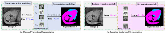
Figure 1.
Classical variational image segmentation and model-inspired learning method. (a) The first stage solves the nonlinear differential equations using the classical iterative method, and then, the second stage thresholds the smooth solution in the first stage to extract objects. (b) The first stage learns the solution mapping by optimizing the convolution kernel to extract image features. The second stage learns the feature fusion and segmentation thresholding parameter.
It is well known that the solution usually has the multiscale property, so a natural idea is to exploit the multi-layer convolution and multigrid architecture, which can describe multiscale features to learn . Based on the above facts, we propose a two-stage segmentation framework for learning feature in Stage 1 and segmentation in Stage 2, which is shown in Figure 1b.
1.2. Contributions
In this work, we focus on analyzing the feature extraction inverse problem (2) and the feature fusion segmentation (3) to design an explainable deep learning network. It is well known that the unrolled iterations of the classical solution algorithm can be considered as the layers of a neural network, so we propose a novel FAS-driven UNet (FAS-UNet), which integrates image data and a multiscale algorithm for solving the nonlinear inverse problem (7). The major differences with our approach are that MgNet is not a U-shaped architecture and is only used for image classification, which leads to the output result not being able to be converted to the segmentation prediction of the input image. Besides, the proposed network was inspired by the traditional multiphase convexity Mumford–Shah variational model [30] and FAS algorithm for solving nonlinear systems [33], which exploits the model and algorithm priors’ information to extract the image features. Indeed, the goal of our work is to show that, under some assumptions about the operators, it is possible to interpret the smoothing operations of the FAS and image geometric extracting operations of the variational model as the layers of a CNN, which in turn, provide fairly specialized network architectures that allow us to solve the standard nonlinear system (7) for a specific choice of the parameters involved.
Our main contributions are summarized as follows:
- We propose a novel variational-model-informed two-stage image segmentation network (FAS-UNet), where an explainable and lightweight sub-network for feature extraction is designed by combining the traditional multiphase convexity Mumford–Shah variational model and FAS algorithm for solving nonlinear systems. To the best of our knowledge, it is the first unrolled architecture designed based on model and algorithm priors in the image segmentation community.
- The proposed model-informed network integrates image data and mathematical models, and it provides a helpful viewpoint for designing the image segmentation network architecture.
- The proposed architecture can be trained from additional model information obtained by enforcing some of the mathematical and physical laws for better accuracy, faster training, and improved generalization. Extensive experimental results show that it performs better than the other state-of-the-art methods.
2. Variational Segmentation via the CNN Framework
The goal of image segmentation is to partition a given image into r regions that contain distinct objects and satisfy , and , where the image domain is a bounded and open subset of . Assume that is the union of boundaries of , denoting the arc length of curve .
2.1. Multiphase Variational Image Segmentation
As mentioned, various ways of variational image segmentation have been proposed. Below, we review a few of them.
2.1.1. Variational Image Segmentation
The Mumford–Shah (M-S) model is a well-known variational image segmentation method proposed by Mumford and Shah [34], which can be defined as follows:
where and are the weight parameters. The first term requires that approximates f, the second term that u does not vary much on each , and the third term that the boundary is as short as possible. This shows that u is a piecewise smooth approximation of f.
In particular, Chan and Vese considered the special case of the M-S model where the function u is chosen to be a piecewise constant function; thus, the minimization for two-phase segmentation is given as
where and are the average image intensities inside and outside of boundary , respectively, and and are the weight parameters.
Sometimes, the given image is degraded by noise and problem-related blur operator . Therefore, Cai et al. [30] extended the two-stage image segmentation strategy using a convex variant of the Mumford–Shah model as
where and are positive parameters, and the existence and uniqueness of u were analyzed in their work.
We assume the image features , where is a smooth mapping defined on the tissue or lesion . In this work, we extend the above model (4) to the multiphase case, which can deal with d-phase segmentation (multiple objects), which refers to a two-stage composite process of feature extraction (6) and feature fusion segmentation (3).
2.1.2. Feature Extraction
The first stage is to extract image features by maximizing a posterior probabilistic distribution (6) for feature representations of a given image f as
where is the environmental parameter in classical “unconscious inference” or the inverse problem. Especially, the likelihood probability and the prior probability can be modeled as normal distributions, respectively, denoted by
thus, the first stage is to find a smooth approximation by minimizing the multiphase generalizability (TS-MCMS) of (4), which can be rewritten as
where is a convolutional blur operator, is a geometric prior of , and . Hence, this leads to the nonlinear system as
where and .
2.1.3. Feature Fusion Segmentation
Once the features are obtained, the segmentation is performed by fusing properly in the second stage; for example, many novel image segmentation methods [30,31,32] have been proposed based on thresholding the smooth solution . Then, the fusing process for feature is finished in (3).
The model-driven methods introduce prior knowledge regarding many desirable mathematical properties of the underlying anatomical structure, such as phase field theory, -approximation, smoothness, and sparseness. The informed priors may help to render the segmentation method more robust and stable. However, these model-inspired methods generally solve the optimization problem in the image domain, while the numerical minimization method for the feature representations is very slow because the regularization of the TV-norm, the high dimensionality of , as well as the nonlinear relationship between the images and the parameters pose significant computational challenges. Furthermore, it is challenging to introduce priors flexibly under different clinical scenes. These limitations make it hard for purely model-based segmentation to obtain the solutions efficiently and flexibly.
2.2. Proposed Learnable Framework of TS-MCMS Algorithm
We summarized the two-stage algorithm to formulate medical image segmentation based on the TS-MCMS model, inspired by the CNN architectures of unrolled iterations, and we propose a learnable framework with two CNN modules on multiscale feature spaces, FAS-UNet (see Figure 1b), aimed at learning the nonlinear inverse operators of (7) and (3) in the context of the variational inverse problem to segment a given image f.
It is already well known that the unrolled iterations of many classical algorithms can be considered as the layers of a neural network [22,23,24,25,26]. In this part, we are not interested in designing another approach for inferring the classes in MgNet [27], but rather, we aim at extracting the features of a given image f.
Inspired by the variational segmentation model (6), one of the key ideas in the proposed architecture is that we split our framework into a solution module and a feature fusion module , where is the feature extraction part of the framework (in the multi-stage case) and is the stage fusion part to be learned. Therefore, how to design the effective function maps for approximately solving (7) and for approximating (3) is an important problem.
This work applies a nonlinear multigrid method to design FAS-UNet for explainable medical image segmentation by learning the two following modules:
where f is an input image, is the feature maps, and is the prediction for the truth partitions, leading to the overall approximation function as
where and are parameters to be learned in the proposed explainable FAS-UNet architecture.
To understand the approximation ability of the proposed modules and generated by the FAS-UNet architecture, we refer the readers to D. Zhou’s work [35], which answers an open question in CNN learning theory about how deep CNN can be used to approximate any continuous function to an arbitrary accuracy when the depth of the neural network is large enough.
2.3. FAS-Module for Feature Extraction
In this part, we discuss how the multigrid method can be used to solve nonlinear problems. The Helmholtz Hypothesis [29] demonstrates that the extracted features can also be represented by solving the equation:
subject to
where denotes the transformation of combining feature with a deblurred image , is the unknown features, and is the ground-truth of image f. Our starting point is the traditional FAS algorithm solving (10).
2.3.1. The Full Approximation Scheme
The multigrid method is usually used to solve nonlinear algebraic systems (10). For simplicity, the parameter in is omitted when only the classical FAS algorithm is involved, i.e.,
The multigrid ingredients including the error smoothing and the coarse grid correction ideas are not restricted to the linear situation, but can be immediately used for the nonlinear problem itself, which leads to the so-called FAS algorithm. The fundamental idea of the nonlinear multigrid is the same as in the linear case, and the FAS method can be recursively defined on the basis of a two-grid method. We start with the description of one fine–coarse cycle (finer grid layer ℓ and coarser grid layer ) of the nonlinear two-grid method for solving (11). To proceed, let the fine grid equation be written as
Firstly, we compute an approximation of the fine grid problem by applying m pre-smoothing steps to as follows
- ;
- fordo
- end for
- ,
which can be obtained via solving the least-squares problem defined by
Secondly, the errors to the solution have to be smoothed such that they can be approximated on a coarser grid. Then, the defect is computed, and an analog of the linear defect equation is transferred to the coarse grid, which is defined by
The coarse grid corrections are interpolated back to the fine grid by
where is a solution of the coarse grid equations, then the errors are finally post-smoothed by
- ;
- fordo
- end for
- .
This means that, once the solution of the fine grid problem is obtained, the coarse grid correction does not introduce any changes via interpolation. We regard this property as an essential one, and in our derivation of the coarse grid optimization problem, we make sure that it is satisfied.
2.3.2. FAS-Solution Module—A Learnable Architecture for FAS Solution
In this part, we unroll the multiscale correction process of the multigrid method and design a series of deep FAS-Solution modules to propagate the features of input image f. Figure 2 demonstrates the cascade of all ingredients at each FAS iteration of our propagative network.
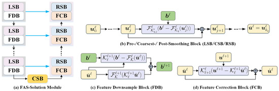
Figure 2.
The overall flowchart of the proposed feature extraction module (FAS-Solution module) with the multigrid architecture. It consists of three major ingredients, i.e., pre-/coarsest-/post-smoothing blocks (LSB/CSB/RSB), feature downsample block (FDB), and feature correction block (FCB).
We now consider a decomposition of the image representation into partial sums, which correspond to the multiscale feature sequence, having the following idea in mind. To learn features that are invariant to noise and uninformative intensity variations, we propose a generative feature module allowing for a significant reduction of the number of parameters involved, which involves a learnable FAS update for solving the nonlinear system (10). Next, we analyze its three key components as follows.
Pre-/coarsest-/post-smoothing block: Error smoothing is one of the two basic principles of the FAS approach. At each pre-smoothing (or coarsest-processing or post-processing) step, to establish an efficient error correction and reduce the computational costs, we propose to generate the error-based iterative scheme. The main motivation of the learnable pre-/coarsest-/post-smoothing blocks (LSB/CSB/RSB) is to provide another way to robustly resolve the ambiguity of the feasible solutions. Therefore, we further unroll the Newton update process for calculating the approximate solution of the feature maps, then design a series of deep pre-/coarsest-/post-smoothing blocks as
- fordo
- end for
- ;
where the residual network block is a trainable feature correction network; here, with -grid cycles. The above deep smoothing series denotes the pre-smoothing block when , the coarsest-smoothing when , and the post-smoothing when . (or , which means that the convolution will share the same weights in the overall pre-/post-precessing smoothing steps of the grid cycle) represents operations consisting of three main components, including convolution (or ) with p filters, ReLU function , and batch normalization , such that . Especially, is an initial feature in the finest grid, which is obtained by learning the convolution with p filters.
Feature downsample block: The choice of restriction and interpolation operators and in the FAS algorithm, for the intergrid transfer of grid functions, is closely related to the choice of the coarse strategy. Here, we design the learnable convolution for transfer operators, i.e., the grid transfers between the finer grid ℓ and the coarser grid .
The low-frequency components represent meaningful image features on a coarse grid , whereas the high-frequency components do not because they are not “visible” on the coarse grid, which means that the frequency information on the coarse grid can be extracted from the right-side term defined by
where and are the inputs of the downsample block and is the output of the downsampling module in the feature space; here, with -grid cycles. Similar to , is a learnable downsample operation that would be used to approximate the restriction function in (12) or (13), such as convolution with a stride of 2 and p filters. and are the nonlinear convolutional blocks in the fine and coarse layers, respectively. In general, denotes the operator consisting of three main components, including convolution with p filters, ReLU function , and batch normalization , such that . Note that is equivalent to the residual of the images in the fine layer, then is added to reduce the loss of image information compared with directly pooling the image. The feature downsample block (FDB) architecture is shown in Figure 2b.
Feature correction block: The purpose of the feature correction block (FCB) is to take the detailed information extracted from the coarser grid into account and help to compensate the encoded features . The coarse grid corrections are interpolated back to the fine grid, i.e.,
where is a learnable upsampling operation that would be used to approximate the interpolation function in (13), such as the transposed convolution with a stride of 2 and p filters; here, with -grid cycles. Obviously, is the residual features on the coarse grid. Compared to directly upsampling , the transposed convolution of the residual feature maps is used as the error corrections to update the fine grid approximation , which will compensate the information of feature maps . Such a transposed convolution could learn a self-adaptive mapping to restore features with more detailed information.
Based on these designs for nonlinear operator and two grid transfer convolutions and with p filters, we aimed to approximate the feature solution of (6) by learning these feature extraction parameters as
in , thus further improving image segmentation.
2.4. Learning Feature Fusion Segmentation
It is well known that, in the segmentation task, each pixel is labeled as either 0 or 1 so that organ pixels can be accurately identified within the tight bounding box. In the second stage of the two-stage multiphase variational image segmentation (6), the traditional method is that users manually set one or more thresholds according to their professional prior, with all pixels in the same object sharing the threshold, and then, filter the feature to obtain the segmentation result. Another method is to obtain the final segmentation result by k-means clustering (the number of categories is given artificially, and the initial clustering center is adjusted continuously during the clustering process) [30]. This approach leads to a large amount of computation (recalculation of the metrics for each iteration) and unstable segmentation results (only considering the relationship between pixels and centers, not the relationship between pixels).
The second key component of our proposed FAS-UNet framework is how to design the segmentation module to compute segmented mask . However, the fusion segmentation module takes a batch of multiscaled features from the FAS module as the input and outputs the mass segmentation masks. Finally, the pixel segmentation computes the mapping from smaller-scale possibility predictions to binary masks.
Based on this idea, the feature fusion segmentation module is constructed, which comprises a convolutional operation and an activation function. Intuitively, the module of the feature extraction based on deep learning obtains the multi-channel feature maps (much larger than the number of categories) in the first stage. Then, a shallow convolutional network is constructed to learn the parameters corresponding to the mapping from the feature maps to the segmentation probability maps through softmax function , which improves the traditional practice and has better generalization.
Based on these designs for channel transfer convolution with c filters (c is the number of segmentation categories), we aimed to approximate the final multiphase segmentation probability maps of (6) by learning these fusion parameters as
in , thus further refining the segmentation mask.
2.5. Loss Function
The proposed FAS-UNet architecture can be rewritten as
which requires the loss function to optimize the model parameters . It can measure the error between the prediction and labels, and the gradients of the weights in the loss function can be back-propagated to the previous layers in order to update the model weights.
To proceed, we considered the training data from a set of classes used for training a pixel classifier, where is an image sample, is the corresponding label, c is the number of object categories segmented in the datasets, d indicates the number of image pixels, and n denotes the number of training samples. We employed the cross-entropy as the loss function, leading to the optimization problem as follows:
where denotes the predicted probabilistic vector of the pixel in the sample and corresponds to the one-hot-encoded label of the ground-truth at the pixel in the sample. . Finally, the predicted class of the pixel of the image would be given by
where .
3. Datasets and Experiments
In this section, we first introduce the evaluation metrics for medical image segmentation and also describe the datasets and the experimental settings that we used for 2D CT image segmentation and 3D medical volumetric segmentation. Next, we analyzed the sensitivity of 2D FAS-UNet to each hyperparameter configuration by a series of experiments. Finally, we evaluated the effectiveness of the proposed 2D/3D FAS-UNet through comparative experiments.
3.1. Evaluation Metrics
There are many metrics to quantitatively evaluate segmentation accuracy, each of which focuses on different aspects. In this work, we employed the average Dice similarity coefficient (a-DSC), average precision (a-Preci), and average symmetric surface distance (a-SSD), which are widely used in the segmentation task as evaluation metrics to evaluate the performance of the model. The a-DSC/a-Preci/a-SSD are calculated by averaging the DSC/Preci/SSD of each category [36].
The Dice score is the most-used metric in validating medical image segmentation, also called the DSC score [37], defined by
where S and Y denote the automatically segmentation set of images and the manually annotated ground-truth, respectively. denotes the measure of a set. The above formulas compute the overlap between the prediction and the ground-truth, to evaluate the overall effect of the segmentation results. However, it is fairly insensitive to the precise boundary of the segmented regions. Precision effectively describes the purity of the prediction relative to the ground-truth or measures the number of those pixels actually having a matching ground-truth annotation by calculating
where a true positive (TP) is observed when a prediction–target mask pair has a score that exceeds some predefined threshold and a false positive (FP) indicates that a predicted object mask has no associated ground-truth. The SSD value between two finite point sets S and Y is defined as follows:
where denotes the minimum Euclidean distance from point v to all points of X.
3.2. Datasets and Experimental Setup
We evaluated the proposed method and other state-of-the-art methods on the 2D SegTHOR datasets [38], 3D HVSMR-2016 datasets [39], and 3D CHAOS-CT datasets [40,41], respectively. We introduce their details and data processing methods as follows.
3.2.1. Data Preparation
For the SegTHOR datasets, in order to reduce the GPU memory cost and reduce the image noise, we first split the original 3D data into many 2D images along the Z-axis. Secondly, we used as the input image, where denotes the original 2D slice. We removed the slices of the pure black ground-truth when it was in training on the datasets.
For the 3D HVSMR-2016 datasets, we directly used the sliding window cropping method with strides of to crop the volumes. In general, before cropping the 3D whole-volume into several overlapping sub-volumes of size , a -voxel padding with zero filling was first added to each direction of the 3D whole-volume. Then, after these operations, all remaining sub-volumes whose sizes were smaller than were resized to with zero-filling, and the intensity values of all patches were in .
For the 3D CHAOS-CT datasets, which were used as for the liver segmentation experiments, we first cropped the volumes in the directions to obtain an ROI with a size of and then used the above sliding window cropping method to crop out several 3D sub-volumes, where those intensity values were in .
Although the noise problem can be improved by data pre-processing, our aim was not to pursue the best performance of the network on these datasets; we compared the performance of each method under fairer conditions. Using some data pre-processing techniques may be particularly beneficial to some methods, while at the same time, they may degrade the performance of others, so we did not use more complex data pre-processing techniques.
3.2.2. Experimental Configurations
We used mini-batch stochastic gradient descent (SGD) to optimize the proposed model, in which the initial learning rate, momentum parameter, and weight decay parameter were set to 0.01, 0.99, and , respectively. We set the batch size as 16, 4, and 4 for the 2D SegTHOR datasets, 3D HVSMR-2016 datasets, and 3D CHAOS-CT datasets, respectively. The maximum epochs of the three datasets were set to 150, 150, and 300, respectively. We used also the decay strategy to update the learning rate. The network initialization method was defined as Kaiming initialization, and the activation function was set as ReLU. The numbers of grid cycles for 2D and 3D FAS-UNet were and , respectively. The kernel sizes of the 2D and 3D networks were set to and as the defaults, respectively. We did not use the weight-sharing scheme for the convolution (within the outer-level nonlinear operator ) within one smoothing block. Table 1 shows the details of the 2D FAS-UNet framework, and 3D FAS-UNet has a similar architecture, except for replacing the 2D convolution with a 3D convolution.

Table 1.
A standard configuration of the proposed 2D FAS-UNet. denotes the number of channels and the height and width of the feature maps, respectively. “conv3, s = 1 or 2” indicates the convolution with a kernel size of and the stride of convolution being 1 or 2, respectively. ReLU and BN are the ReLU activation function and batch normalization.
3.2.3. Parameter Complexity
To compute the number of parameters of the proposed model, we first denote the number of parameters of 2D convolution kernel with the shape as follows:
Similarly, the number of parameters of 3D convolution with the shape is defined as
Especially if the channel ratio satisfies that , one has . Thus, the number of parameters of convolution kernel set in the proposed FAS-UNet can be computed by
where c is the channel number of the input image and is the number of parameters of each 2D or 3D convolution .
If setting , , and , one has ; hence, 2D FAS-UNet has approximately parameters. In addition, one also has when . If setting and , thus 3D FAS-UNet has approximately parameters. Here, we did not compute , where a small amount of parameters are involved.
Our experiments were implemented on the PyTorch framework and two NVIDIA Geforce RTX 2080Ti GPUs with 11GB memory. For each quantitative result in the experiments, we repeated the experiment twice and chose the best one to compute the mean/std. Note that we used the same pipeline for all these experiments of each dataset for a fair comparison. The networks under comparison were trained from scratch.
3.3. Ablation Studies
We conducted four groups of ablation studies on the 2D SegTHOR datasets to optimize the hyperparameter configurations of the proposed framework.
3.3.1. Blocks’ Sensitivity
Firstly, we assessed the effect of smoothing block configurations , where denote the , , and smoothing iterations in the LSB, CSB, and RSB, respectively. Here, we first fixed the channel configuration with as the default. Table 2 shows a quantitative results of different block parameter sets, and we observed from the pre-smoothing experiments (fixing and , varying ) that 2D FAS-UNet with iterations achieved the best a-DSC score and precision of 85.60% and 85.99%, respectively. For the post-smoothing (fixing and , varying ), we saw that the model with iterations achieved the highest values of a-SSD and precision, the a-DSC score being slightly lower than the model with the block configuration by 0.04%. To balance the prediction performance and computational costs, we set the block configuration as in all 2D experiments.
Table 2.
Quantitative assessment with the a-DSC, a-SSD, and a-Preci values of different pre-/coarest-/post- smoothing iteration numbers using the proposed 2D FAS-UNet framework on the 2D SegTHOR validation datasets with four organs: esophagus, heart, trachea, and aorta. “Mean” denotes an average score segmenting all organs. The best and second places are highlighted in bold font and underline, respectively.
3.3.2. The Input Feature Initialization
We also evaluated the initialization configuration of the input feature on the finest cycle to verify its sensitivity. We compared different variants of the initialization method, such as zero initialization, random normal distribution initialization, and initialization with the batch normalization operation , where was obtained by learning the convolutional kernel with a size of for 2D segmentation or for 3D segmentation.
Table 3 shows the quantitative comparison of these variants. The model with initialization achieved a-DSC, a-SSD, and a-Preci values of 85.58% (ranked second), 2.61 mm (top-ranked), and 89.75% (top-ranked), respectively. Although the model with random initialization had the highest a-DSC score, the a-SSD and a-Preci scores were significantly lower than the model with initialization. To this end, we set the proposed framework with initialization as the default in this work.
Table 3.
Quantitative assessment with the a-DSC, a-SSD, and a-Preci values of different initialization techniques (zero initialization, random initialization, and feature extraction initialization using the proposed 2D FAS-UNet framework on the 2D SegTHOR validation datasets with four organs: esophagus, heart, trachea, and aorta. “Mean” denotes an average score segmenting all organs. The best and second places are highlighted in bold font and underlined, respectively.
3.3.3. Weight Sharing
To demonstrate the flexibility of the proposed framework, which does not have to be the different parameter configurations in different nonlinear (with respect to j) within the pre-smoothing () or post-smoothing () block, we conducted several variants that had different sharing settings among (with respect to the iteration step j).
We only varied the weight sharing settings to verify the sensitivity of the model. We compared four variants, and the results are shown in Table 4. From the evaluation metrics, we see that the model without the weight sharing configuration had moreparameters and achieved the best performance on the a-DSC, a-SSD, and a-Preci values, respectively. The performance of the other three models did not show a significant differences. Therefore, we adopted the default unshared version in the rest of this paper.
Table 4.
Quantitative assessment with the a-DSC, a-SSD, and a-Preci values of using the proposed 2D FAS-UNet framework with/without weight sharing of pre-/post smoothing steps on the 2D SegTHOR validation datasets with four organs: esophagus, heart, trachea, and aorta. “Mean” denotes an average score segmenting all organs. The best and second places are highlighted in bold font and underlined, respectively.
3.3.4. Effects of Varying the Number of Channels
In this section, we analyze the segmentation performance of the proposed method with varying the number p of feature channels. In the FAS-Solution module, the pre-smoothing and post-smoothing steps (with and iterations, respectively) had the same update structure with the coarsest smoothing step, which included iterations. Therefore, we set the number of smoothing iterations as and adopted a series of channel parameters , respectively, for comparison. Here, means that, in each convolutional operation of the FAS-Solution module, there were 80 filters with the same kernel size of .
Table 5 shows the quantitative comparison of different p-configurations. It reveals that, as the number of channels increased, the parameter of our model squarely increased. Additionally, the networks with the numbers of 64 and 16 achieved a-DSC scores of 86.83% (ranking first) and 84.88% (ranking lowest), respectively. When the number of channels was less than 64, increasing the number of channels could improve the a-DSC value, and one can see from Table 5 that the number of channels had a significant impact on the performance of the model. Based on this observation, the configuration with 64 channels is a preferable setting to balance the segmentation performance and computational costs, and we fixed throughout all the 2D experiments.
Table 5.
Quantitative assessment with the a-DSC, a-SSD, and a-Preci values of different channel numbers p using the proposed 2D FAS-UNet framework on the 2D SegTHOR validation datasets with four organs: esophagus, heart, trachea, and aorta. “Mean” denotes an average score segmenting all organs. The best and second places are highlighted in bold font and underlined, respectively.
To provide insights into the model hyperparameter configurations of the proposed 3D FAS-UNet version on the 3D HVSMR-2016 datasets and 3D CHAOS-CT datasets, we also carried out a series of ablation experiments to investigate the influence of two key design variables, the number of channels and the number of convolutional blocks. The evaluation indicated that the network performed better with the configurations , for the 3D HVSMR-2016 datasets and for the 3D CHAOS-CT datasets as the default. Here, we do not detail these comparisons.
Finally, we illustrate the hyperparameter configurations of the proposed FAS-UNet on each dataset throughout all experiments, as shown in Table 6.
Table 6.
The hyperparameter configurations of the proposed FAS-UNet framework on different datasets.
3.4. The 2D FAS-UNet for the SegTHOR Datasets
We evaluated the proposed network on the 2D SegTHOR datasets and compared the visualizations and quantitative metrics with the existing state-of-the-art segmentation methods, including 2D UNet [9], CA-Net [20], CE-Net [42], CPFNet [43], ERFNet [44], UNet++ [11], and LinkNet [45].
In Table 7, we show the quantitative results of each organ’s segmentation compared with the other seven models. We can see that the segmentation performance of the heart was the best among all organs, and its a-DSC score was more than 92% for each method, followed by the aorta, and the worst was the esophagus. The main reason for the good performance in extracting the heart was that the heart region is the largest, and its inner pixel value changes little, while its boundary is more obvious (see Figure 3), while the esophageal region is the smallest among all organs, which increased the segmentation difficulty.
Table 7.
Performance comparisons between the proposed 2D FAS-UNet and the popular networks using the a-DSC, a-SSD, and a-Preci values on the 2D SegTHOR validation datasets with four organs: esophagus, heart, trachea, and aorta. “Mean” denotes an average score segmenting all organs. The best and second places are highlighted in bold font and underlined, respectively.
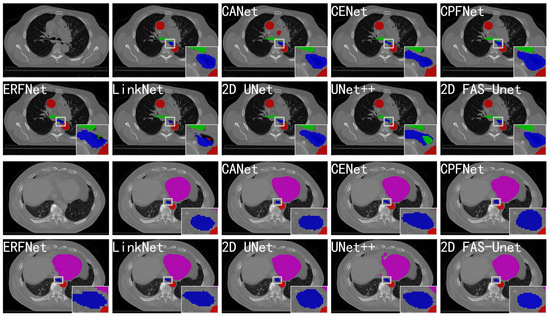
Figure 3.
Comparison with the other state-of-the-art networks on the validation set of the 2D SegTHOR datasets. The blue, pink, green, and red regions represent the esophagus, heart, trachea, and aorta, respectively. Form left to right in the first and third rows: the original images, ground-truth, and segmentation results of CANet, CE-Net, and CPFNet, respectively. Form left to right in the second and fourth rows: the segmentation results of ERFNet, LinkNet, 2D UNet, UNet++, and 2D FAS-UNet, respectively.
The proposed method achieved an a-DSC value of 86.83% (ranked first) and an a-Preci value of 88.21% (ranked first) with only 2.08 M parameters. Compared with the state-of-the-art models CA-Net (second-ranked in the a-DSC score) and UNet++ (ranked second in the a-Preci value), the proposed 2D FAS-UNet obtained a 0.17% improvement of the a-DSC score with only 75% as many parameters as CA-Net and a 0.19% improvement of the a-Preci value with only 22% as many parameters as UNet++. Our method also had a higher a-DSC score than the third-ranked UNet by 0.75%, but had far fewer parameters than the 17.26 M of UNet. Compared with ERFNet, which achieved a-DSC and a-Preci values of 82.86% and 80.48% with the fewest parameters, respectively, FAS-UNet was higher in the overall a-DSC rankings. The a-DSC score of ERFNet ranked last, so we think it may fall into an under-fitting situation. This shows that ERFNet reduces the performance of the network while saving the parameters. CA-Net obtained a good a-DSC value because the attention mechanism may improve the segmentation results of small organs.
The evaluation results were also measured in terms of the a-SSD value for segmentation predictions of the eight methods. The proposed method achieved an a-SSD value of 5.19 mm (ranked fourth); CE-Net ranked first, which achieved an a-SSD value of 4.08 mm; ERFNet with the fewest parameters ranked fifth with 5.92 mm. CA-Net and Link-net ranked second and third, which had 2.78 M and 21.79 M parameters, respectively. The good results of CA-Net in terms of the a-SSD metric may be due to the use of multiple attention mechanisms, which enables the network to suppress the background region, and the network has a stronger ability to recognize the object region. The a-SSD score of UNet++ was much higher than that of 2D FAS-UNet, which shows that the over-segmented pixels were less than the under-segmented pixels. Meanwhile, we observed that the a-SSD value of our method was close to that of LinkNet in three organs; only the tracheal region was significantly worse than it, which makes it better than our method in the mean a-SSD score.
Figure 3 evaluates the visualizations of the segmented predictions obtained by the popular methods. One can observe that all methods except CA-Net (with an obvious over-segmentation) can accurately segment the aortic region (red). The reason may be that, during the imaging process, the aortic organ may be assigned to the very same image pixel, which leads to a small difference of the internal pixel value; in particular, the network can accurately learn its features. Almost all methods can also approximately segment the trachea organ shape (green); only the organ boundary is not clearly visible. This may be a common problem in small object segmentation because the hard-to-detect small-scale feature will be degraded rapidly with convolution and pooling. All methods were able to extract the heart location (magenta), while the visual quality of the proposed method was significantly better than the state-of-the-art methods. Our approach achieved the least missing pixelsat the organ boundary, which resulted in substantially better performance than the existing results; the visualization remained comparable. It should also be emphasized that only a few methods performed well on the left boundary because the left side of the heart’s boundary is very blurry. For example, UNet++ presented over-segmentation, and CA-Net on the left boundary was significantly different from the ground-truth, while the results of ERFNet and LinkNet had significant differences compared with the ground-truth in the shape aspect. This also shows that our method is robust to the heavy occlusion of illumination and large background clutters.
For the esophagus organ (blue) in Figure 3, the segmented results of CE-Net, CPFNet, and UNet had significantly differences compared with the ground-truth in the shape aspect. The results of ERFNet and UNet++ had some trachea pixels within the esophagus, and LinkNet’s prediction had some aortic pixels, all of which were clearly error-segmented. The predictions of CA-Net and FAS-UNet were similar to manual segmentation, but the result of CA-Net had a small aorta patch in the background region, while our method obviously performed better. The reasons for the esophagus’s bad results were the fuzzy boundary and the small pixel value difference; in particular, the esophagus and aorta almost overlap in the second slice. Therefore, the proposed method is more robust, and it is more difficult for it to be affected by noise. This further shows that our method is effective in medical image segmentation.
3.5. The 3D FAS-UNet for the HVSMR-2016 Datasets
We also conducted the segmentation experiments of our 3D FAS-UNet on the HVSMR-2016 datasets. We compared our predictions with seven baseline models including 3D UNet [46], AnatomyNet [47], DMFNet [48], HDC-Net [49], RSANet [50], Bui-Net [51], and VoxResNet [52]. Table 8 shows the segmentation results of different methods. Clearly, our method with fewer parameters ranked second in both the a-DSC and a-SSD values and obtained the top rank in mean precision.
Table 8.
Performance comparisons of the proposed 3D FAS-UNet and the popular networks using the a-DSC, a-SSD, and a-Preci values on the 3D HVSMR-2016 validation datasets with both organs: myocardium and blood pool. “MY” and “BP” denote myocardium and blood pool, respectively, “Mean” denotes an average score segmenting all organs. The best and second places are highlighted in bold font and underlined, respectively.
The proposed method achieved an a-DSC value of 82.75% (ranked second) with only 1.01 M parameters and followed the first-ranked 3D UNet by 0.1% in the a-DSC score with only 15% as many parameters as 3D UNet. Meanwhile, our method outperformed the third-ranked DMFNet by 2.84%. Although the numbers of parameters of HDC-Net and AnatomyNet were lower than that of our method, the a-DSC score of 3D FAS-UNet was 3.82% and 4.96% higher than theirs, respectively. One may notice that a black-box (unexplainable) network with a small number of parameters has low segmentation performance, which may be due to under-fitting. However, the number of parameters in RSANet is a bit large, and the effect was also not good enough. This may be due to too little training data, so the model appears to be over-fitting. Our method also obtained an a-SSD value of 2.44 mm (2nd rank), which was lower than DMFNet’s 2.40 mm (1st rank) by 0.12 mm, and it slightly improved compared with 3D UNet, whose a-SSD value was 2.56 mm (3rd ranked). Although 3D FAS-UNet had a slightly lower a-SSD than DMFNet, it had 2.86 M fewer parameters. Compared with HDC-Net and AnatomyNet with fewer parameters, our method performed better on the a-SSD metric for myocardium and blood pool. The result of the a-SSD value shows that our method has good performance in segmenting object boundaries. The proposed method obtained the best a-Preci score of 87.90%, which was higher than the second-ranked Bui-Net by 1.10%. Although 3D FAS-UNet ranked third in the number of parameters, all three metrics were better than HDC-Net and AnatomyNet with fewer parameters. Therefore, our method achieves a good balance between the number of parameters and performance. Experiments on these datasets showed that the proposed FAS-driven explainable model can be robustly applied to 3D medical segmentation tasks.
Figure 4 visualizes the segmentation results of different methods on two slices of the HVSMR-2016 datasets, and it can be clearly observed that the proposed model highlighted less over-segmented regions outside the ground-truth compared with other methods. Meanwhile, it also can show that it was hard for our method to be affected by the voxels in the background region, where it did not predict the voxels of the background region as blood pools or myocardium, but most other methods predicted more background voxels as the object. The results showed that these methods are easily affected by noise in the background region.
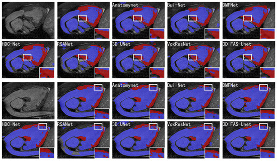
Figure 4.
Visualizations of different methods for cardiovascular MR segmentation of different slices. From left to right in the first and third rows: the original images, the ground-truth, and the segmentation results of AnatomyNet, Skip-connected 3D DenseNet, and DMFNet, respectively. From left to right in the second and fourth rows: the segmentation results of HDC-Net, RSANet, 3D UNet, VoxResNet, and 3D FAS-UNet, respectively. The blue and red colors represent blood pool and myocardium, respectively.
In general, one can observe that AnatomyNet, VoxResNet, and 3D UNet showed obvious segmentation noise (over-segmented region). The reason is that the network collects much noise information in the interactions from input data of the network due to a too simple data pre-processing method, which affects the feature extraction. Several methods presented over-segmentation in the myocardial zoom-in, because the pixel value of this organ is very close to the background. The myocardium is structurally distorted, which makes the shape of the myocardium completely different compared to normal/healthy myocardium. Although VoxResNet did not have this phenomenon, it divided the middle part of the myocardial region into blood pools, which was also an obvious error segmentation. Only 3D UNet and our method performed better; especially, our method was closer to the ground-truth in shape. Further, all methods had poor segmentation results in the upper myocardial region; the intensity homogeneity between this organ and the upper background indicates that this region is very difficult to segment. We can see from the zoom-in results that many methods have obvious over-segmentation or under-segmentation for the myocardium and blood pool. Compared with Bui-Net and RSANet, we observed that the proposed learnable specialized FAS-UNet network still had obvious advantages in this region, and the results were very close to the ground-truth in the myocardial region (red) with respect to the shape and size. For the blood pool region (blue), our results did not show significant differences with other methods.
The proposed network integrates medical image data and the variational convexity MS model and algorithm (FAS scheme), and implements them through convolution-based deep learning, so it may be possible to design specialized modules that automatically satisfy some of the physical invariants for better accuracy and robustness. Qualitative and quantitative experimental results demonstrated the effectiveness and superiority of our method. It can not only correctly locate the position of the myocardium, but also segment the myocardium and blood pool in the complex marginal region. Moreover, the integrity and continuity of our method in the object were well preserved. Overall, it performed better than the existing state-of-the-art methods in 3D medical image segmentation.
3.6. The 3D FAS-UNet for the CHAOS-CT Datasets
In this part, the proposed 3D FAS-UNet was compared with seven baseline models on the 3D CHAOS-CT datasets, including 3D UNet [46], Bui-Net [51], DMFNet [48], 3D ESPNet [53], RSANet [50], RatLesNetV2 [54], and HDC-Net [49].
Firstly, we used a post-processing technique to improve the prediction results, where small undesirable clusters of voxels separated from the largest connection component may be over-segmented or the “holes” inside the liver may also be under-segmented. Table 9 shows the prediction results of different methods. Before post-processing, the proposed method achieved an a-DSC of 96.69% (top-ranked) with only 1.00 M parameters, which is slightly higher than the second-ranked RSANet by 0.08% in the mean a-DSC score with only about 4% as many parameters as RSANet, and further outperformed the third-ranked DMFNet by 0.28%. Our method also obtained an a-SSD value of 4.04mm (ranked second), which is the same as RSANet (top-ranked). Although 3D FAS-UNet had a lower mean a-Preci value than 3D ESPNet by 1.54%, it had 2.57 M fewer parameters.
Table 9.
Performance comparisons of liver segmentation between the different 3D networks with/without post-processing using the a-DSC, a-SSD, and a-Preci values on the 3D CHAOS-CT validation datasets. The best and second places are highlighted in bold font and underlined, respectively.
The a-DSC scores of all methods were significantly improved by post-processing techniques. The 3D FAS-UNet achieved an a-DSC score of 97.11% (ranked second) and followed the first-ranked 3D UNet by 0.05% in the mean a-DSC with only 15% as many parameters as 3D UNet. Our method also obtained an a-SSD value of 1.16 mm (top-ranked), and it was better than 3D UNet (ranked 2nd) and RSANet (ranked 3rd) by 0.07 mm and 0.10 mm, respectively. The 3D FAS-UNet achieved an a-Preci of 96.73%, which is lower than 3D ESPNet and RatLesNetV2. Although 3D FAS-UNet ranked third in the parameter evaluation, all five metrics were better than HDC-Net and RatLesNetV2 with fewer parameters; only the a-Preci value with post-processing was lower than that of RatLesNetV2. Thus, our method achieves a good balance between the number of parameters and segmentation performance.
Figure 5 visualizes the prediction results of different networks on two slices of the CHAOS-CT datasets, and it can be clearly observed that the other networks highlighted more over-segmented regions outside the ground-truth compared with our network. Further, we can observe that the results for Bui-Net, DMFNet, HDC-Net, RatLesNetv2, and RSANet showed obvious segmentation noise in the background region. Although 3D ESP-Net did not present this phenomenon, the result showed an obvious “hole” inside of the liver, which was an obvious error-segmentation. However, our approach did not show these evident inaccurate results. In addition, most methods showed over-segmentation or under-segmentation on the boundaries of liver because it is very blurred in the CT image. From the zoom-in results of the first two rows of Figure 5, we can see that all mentioned methods had obvious under-segmentation except HDC-Net and our method, but our method had less noise in the background region. From the zoom-in results of the last two rows in Figure 5, we observe that many methods showed obvious over-segmentation on the liver boundaries. Only our method and 3D ESPNet achieved a good performance in this region, but 3D ESPNet extracted a “hole” in the liver region. In summary, compared to other methods, the boundary results obtained by our method were smoother, and the shape of the liver was more similar to the ground-truth.
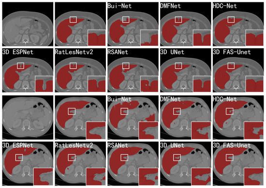
Figure 5.
Visualizations (without post-processing) of different methods for liver CT segmentation of two slices. From left to right in the first and third rows: the original images, ground-truth, the segmentation results of skip-connected 3D DenseNet, DMFNet, and HDC-Net, respectively. From left to right in the second and fourth rows: the segmentation results of 3D ESPNet, RatLesNetv2, RSANet, 3D UNet, and 3D FAS-UNet, respectively.
We show visual comparisons before and after post-processing in Figure 6. The results demonstrated that the “hole” (the first row in Figure 6) was effectively filled, and the “island” (the second row in Figure 6) in the background was removed by post-processing. The experiments indicated that our model-driven approach with post-processing was more effective.
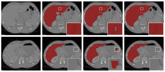
Figure 6.
The segmentation results with post-processing. From left to right: the selected scans of the validation set (first column), ground-truths (second column), segmentation results of 3D FAS-UNet without post-processing (third column), and results with post-processing (fourth column).
Qualitative and quantitative results demonstrated the effectiveness and advantages of the proposed method. Our method achieved a robust and accurate performance compared with the existing state-of-the-art methods in the 3D liver segmentation task, which can be applied to 3D medical image segmentation.
4. Conclusions
In this work, we proposed a novel deep learning framework, FAS-UNet, for 2D and 3D medical image segmentation by enforcing some of the mathematical and physical laws (e.g., the convexity Mumford–Shah model and FAS algorithm), which focuses on learning the multiscale image features to generate the segmentation results.
Compared with other existing works that analyzed the connection between the multigrid and CNN, FAS-UNet integrates medical image data and mathematical models and enhances the connection between data-driven and traditional variational model methodologies; it provides a helpful viewpoint for designing image segmentation network architectures. Compared with UNet, the proposed FAS-UNet introduces the concept of the data space, which exploits the model prior information to extract the features. Specifically, the feature extraction task leads to solving nonlinear equations, and an iterative scheme of numerical algorithms was designed to learn the features. Our experimental results showed that the proposed method is able to improve medical image segmentation in different tasks, including the segmentation of thoracic organs at risk, the whole-heart and great vessel, and liver segmentation. It is believed that the approach is a general one and can be applied to other image processing tasks, such as image denoising and image reconstruction. In addition, we found that the topological interaction module proposed by [55] can effectively improve the performance of many segmentation methods. Therefore, we will use this module in FAS-UNet to improve its performance in the future work.
Author Contributions
Conceptualization, H.Z., S.S. and J.Z.; methodology, H.Z., S.S. and J.Z.; software, H.Z.; validation, H.Z. and J.Z.; formal analysis, H.Z., S.S. and J.Z.; investigation, H.Z., S.S. and J.Z.; resources, H.Z., S.S. and J.Z.; data curation, H.Z.; writing—original draft preparation, H.Z. and J.Z.; writing—review and editing, H.Z., S.S. and J.Z.; visualization, H.Z.; supervision, S.S. and J.Z. All authors have read and agreed to the published version of the manuscript.
Funding
This research was funded by by the National Natural Science Foundation of China (NSFC) under Grants 11971414 and 11771369 and partly by grants from the Natural Science Foundation of Hunan Province (Grants 2018JJ2375, 2018XK2304, and 2018WK4006).
Institutional Review Board Statement
Not applicable.
Informed Consent Statement
Not applicable.
Data Availability Statement
The code and datasets are available at https://github.com/zhuhui100/FASUNet (accessed on 2 October 2022).
Conflicts of Interest
The authors declare no conflict of interest.
References
- Minaee, S.; Boykov, Y.Y.; Porikli, F.; Plaza, A.J.; Kehtarnavaz, N.; Terzopoulos, D. Image Segmentation Using Deep Learning: A Survey. IEEE Trans. Pattern Anal. Mach. Intell. 2022, 44, 3523–3542. [Google Scholar] [CrossRef] [PubMed]
- Boveiri, H.R.; Khayami, R.; Javidan, R.; Mehdizadeh, A. Medical Image Registration Using Deep Neural Networks: A Comprehensive Review. Comput. Electr. Eng. 2020, 87, 106767. [Google Scholar] [CrossRef]
- Cai, L.; Gao, J.; Zhao, D. A Review of the Application of Deep Learning in Medical Image Classification and Segmentation. Ann. Transl. Med. 2020, 8, 713. [Google Scholar] [CrossRef] [PubMed]
- Chen, C.; Qin, C.; Qiu, H.; Tarroni, G.; Duan, J.; Bai, W.; Rueckert, D. Deep Learning for Cardiac Image Segmentation: A Review. Front. Cardiovasc. Med. 2020, 7, 25. [Google Scholar] [CrossRef]
- Litjens, G.; Kooi, T.; Bejnordi, B.E.; Setio, A.A.A.; Ciompi, F.; Ghafoorian, M.; van der Laak, J.A.; van Ginneken, B.; Sánchez, C.I. A Survey on Deep Learning in Medical Image Analysis. Med. Image Anal. 2017, 42, 60–88. [Google Scholar] [CrossRef] [PubMed]
- Miotto, R.; Wang, F.; Wang, S.; Jiang, X.; Dudley, J.T. Deep Learning for Healthcare: Review, Opportunities and Challenges. Briefings Bioinform. 2018, 19, 1236–1246. [Google Scholar] [CrossRef] [PubMed]
- Fu, Y.; Lei, Y.; Wang, T.; Curran, W.J.; Liu, T.; Yang, X. Deep Learning in Medical Image Registration: A Review. Phys. Med. Biol. 2020, 65, 20TR01. [Google Scholar] [CrossRef]
- Liu, X.; Song, L.; Liu, S.; Zhang, Y. A Review of Deep-Learning-Based Medical Image Segmentation Methods. Sustainability 2021, 13, 1224. [Google Scholar] [CrossRef]
- Ronneberger, O.; Fischer, P.; Brox, T. UNet: Convolutional Networks for Biomedical Image Segmentation. In Medical Image Computing and Computer-Assisted Intervention—MICCAI 2015; Springer: Cham, Switzerland, 2015. [Google Scholar]
- Milletari, F.; Navab, N.; Ahmadi, S.A. V-Net: Fully Convolutional Neural Networks for Volumetric Medical Image Segmentation. In Proceedings of the 2016 Fourth International Conference on 3D Vision (3DV), Stanford, CA, USA, 25–28 October 2016; pp. 565–571. [Google Scholar] [CrossRef]
- Zhou, Z.; Siddiquee, M.M.R.; Tajbakhsh, N.; Liang, J. UNet++: Redesigning skip connections to exploit multiscale features in image segmentation. IEEE Trans. Med. Imaging 2019, 39, 1856–1867. [Google Scholar] [CrossRef]
- Cicek, O.; Abdulkadir, A.; Lienkamp, S.S.; Brox, T.; Ronneberger, O. 3D UNet: Learning Dense Volumetric Segmentation from Sparse Annotation. In Proceedings of the Medical Image Computing and Computer-Assisted Intervention—MICCAI 2016: 19th International Conference, Athens, Greece, 17–21 October 2016; Lecture Notes in Computer Science; Ourselin, S., Joskowicz, L., Sabuncu, M.R., Unal, G., Wells, W., Eds.; Springer International Publishing: Cham, Switzerland, 2016; Volume 9901, pp. 424–432. [Google Scholar] [CrossRef]
- Mehta, S.; Mercan, E.; Bartlett, J.; Weaver, D.; Elmore, J.G.; Shapiro, L. Y-Net: Joint Segmentation and Classification for Diagnosis of Breast Biopsy Images. In Medical Image Computing and Computer Assisted Intervention—MICCAI 2018; Frangi, A.F., Schnabel, J.A., Davatzikos, C., Alberola-López, C., Fichtinger, G., Eds.; Springer International Publishing: Cham, Switzerland, 2018; pp. 893–901. [Google Scholar]
- Xiao, X.; Lian, S.; Luo, Z.; Li, S. Weighted Res-UNet for High-Quality Retina Vessel Segmentation. In Proceedings of the 2018 9th International Conference on Information Technology in Medicine and Education (ITME), Hangzhou, China, 19–21 October 2018; pp. 327–331. [Google Scholar] [CrossRef]
- Valanarasu, J.M.J.; Sindagi, V.A.; Hacihaliloglu, I.; Patel, V.M. KiU-Net: Towards Accurate Segmentation of Biomedical Images Using Over-Complete Representations. In Medical Image Computing and Computer Assisted Intervention—MICCAI 2020; Lecture Notes in Computer Science; Martel, A.L., Abolmaesumi, P., Stoyanov, D., Mateus, D., Zuluaga, M.A., Zhou, S.K., Racoceanu, D., Joskowicz, L., Eds.; Springer International Publishing: Cham, Switzerland, 2020; Volume 12264, pp. 363–373. [Google Scholar] [CrossRef]
- Li, X.; Chen, H.; Qi, X.; Dou, Q.; Fu, C.W.; Heng, P.A. H-DenseUNet: Hybrid Densely Connected UNet for Liver and Tumor Segmentation From CT Volumes. IEEE Trans. Med. Imaging 2018, 37, 2663–2674. [Google Scholar] [CrossRef]
- Isensee, F.; Jaeger, P.F.; Kohl, S.A.A.; Petersen, J.; Maier-Hein, K.H. nnU-Net: A Self-Configuring Method for Deep Learning-Based Biomedical Image Segmentation. Nat. Methods 2021, 18, 203–211. [Google Scholar] [CrossRef] [PubMed]
- He, X.; Mo, Z.; Wang, P.; Liu, Y.; Yang, M.; Cheng, J. ODE-Inspired Network Design for Single Image Super-Resolution. In Proceedings of the 2019 IEEE/CVF Conference on Computer Vision and Pattern Recognition (CVPR), Long Beach, CA, USA, 16–20 June 2019; pp. 1732–1741. [Google Scholar]
- Lu, Y.; Zhong, A.; Li, Q.; Dong, B. Beyond Finite Layer Neural Networks: Bridging Deep Architectures and Numerical Differential Equations; StockholmsmÃdssan: Stockholm Sweden, 2018; Volume 80, pp. 3276–3285. [Google Scholar]
- Gu, R.; Wang, G.; Song, T.; Huang, R.; Aertsen, M.; Deprest, J.; Ourselin, S.; Vercauteren, T.; Zhang, S. CA-Net: Comprehensive attention convolutional neural networks for explainable medical image segmentation. IEEE Trans. Med. Imaging 2020, 40, 699–711. [Google Scholar] [CrossRef] [PubMed]
- He, K.; Zhang, X.; Ren, S.; Sun, J. Deep residual learning for image recognition. In Proceedings of the IEEE Conference on Computer Vision and Pattern Recognition, Las Vegas, NV, USA, 27–30 June 2016; pp. 770–778. [Google Scholar]
- Larsson, G.; Maire, M.; Shakhnarovich, G. FractalNet: Ultra-Deep Neural Networks without Residuals. In Proceedings of the ICLR, Toulon, France, 24–26 April 2017. [Google Scholar]
- Zhang, X.; Li, Z.; Change Loy, C.; Lin, D. Polynet: A pursuit of structural diversity in very deep networks. In Proceedings of the IEEE Conference on Computer Vision and Pattern Recognition, Honolulu, HI, USA, 21–26 July 2017; pp. 718–726. [Google Scholar]
- Gomez, A.N.; Ren, M.; Urtasun, R.; Grosse, R.B. The reversible residual network: Backpropagation without storing activations. arXiv 2017, arXiv:1707.04585. [Google Scholar]
- Chen, R.T.; Rubanova, Y.; Bettencourt, J.; Duvenaud, D. Neural ordinary differential equations. arXiv 2018, arXiv:1806.07366. [Google Scholar]
- Yang, Y.; Sun, J.; Li, H.; Xu, Z. Deep ADMM-Net for Compressive Sensing MRI. In Proceedings of the Advances in Neural Information Processing Systems 29: Annual Conference on Neural Information Processing Systems 2016, Barcelona, Spain, 5–10 December 2016; Lee, D.D., Sugiyama, M., von Luxburg, U., Guyon, I., Garnett, R., Eds.; Curran Associates, Inc.: Red Hook, NY, USA, 2016; pp. 10–18. [Google Scholar]
- He, J.; Xu, J. MgNet: A unified framework of multigrid and convolutional neural network. Sci. China Math. 2019, 62, 1331–1354. [Google Scholar] [CrossRef]
- Alt, T.; Schrader, K.; Augustin, M.; Peter, P.; Weickert, J. Connections between numerical algorithms for PDEs and neural networks. arXiv 2021, arXiv:2107.14742. [Google Scholar] [CrossRef]
- Heyer, D.; Mausfeld, R. Perception and the Physical World: Psychological and Philosophical Issues in Perception; John Wiley & Sons, Ltd.: New York, NY, USA, 2002. [Google Scholar]
- Cai, X.; Chan, R.; Zeng, T. A Two-Stage Image Segmentation Method Using a Convex Variant of the Mumford–Shah Model and Thresholding. SIAM J. Imaging Sci. 2013, 6, 368–390. [Google Scholar] [CrossRef]
- Liu, C.; Ng, M.K.P.; Zeng, T. Weighted Variational Model for Selective Image Segmentation with Application to Medical Images. Pattern Recognit. 2018, 76, 367–379. [Google Scholar] [CrossRef]
- Ma, Q.; Peng, J.; Kong, D. Image Segmentation via Mean Curvature Regularized Mumford–Shah Model and Thresholding. Neural Process. Lett. 2018, 48, 1227–1241. [Google Scholar] [CrossRef]
- McCormick, S.F. Multigrid Methods; SIAM: Philadelphia, PA, USA, 1987. [Google Scholar]
- Mumford, D.B.; Shah, J. Optimal approximations by piecewise smooth functions and associated variational problems. Commun. Pure Appl. Math. 1989, 42, 577–685. [Google Scholar] [CrossRef]
- Zhou, D.X. Universality of deep convolutional neural networks. Appl. Comput. Harmon. Anal. 2020, 48, 787–794. [Google Scholar] [CrossRef]
- Taha, A.A.; Hanbury, A. Metrics for evaluating 3D medical image segmentation: Analysis, selection, and tool. BMC Med. Imaging 2015, 15, 29. [Google Scholar] [CrossRef] [PubMed]
- Dice, L.R. Measures of the Amount of Ecologic Association Between Species. Ecology 1945, 26, 297–302. [Google Scholar] [CrossRef]
- Lambert, Z.; Petitjean, C.; Dubray, B.; Kuan, S. SegTHOR: Segmentation of Thoracic Organs at Risk in CT images. In Proceedings of the 2020 Tenth International Conference on Image Processing Theory, Tools and Applications (IPTA), Paris, France, 9–12 November 2020; pp. 1–6. [Google Scholar] [CrossRef]
- Pace, D.F.; Dalca, A.V.; Geva, T.; Powell, A.J.; Moghari, M.H.; Golland, P. Interactive Whole-Heart Segmentation in Congenital Heart Disease. In Medical Image Computing and Computer-Assisted Intervention—MICCAI 2015; Springer: Cham, Switzerland, 2015; Volume 9351, pp. 80–88. [Google Scholar]
- Kavur, A.E.; Gezer, N.S.; Barış, M.; Aslan, S.; Conze, P.H.; Groza, V.; Pham, D.D.; Chatterjee, S.; Ernst, P.; Özkan, S.; et al. CHAOS challenge-combined (CT-MR) healthy abdominal organ segmentation. Med. Image Anal. 2021, 69, 101950. [Google Scholar] [CrossRef] [PubMed]
- Kavur, A.E.; Selver, M.A.; Dicle, O.; Barış, M.; Gezer, N.S. CHAOS—Combined (CT-MR) Healthy Abdominal Organ Segmentation Challenge Data. Zenodo 2019. [Google Scholar] [CrossRef]
- Gu, Z.; Cheng, J.; Fu, H.; Zhou, K.; Hao, H.; Zhao, Y.; Zhang, T.; Gao, S.; Liu, J. CE-Net: Context Encoder Network for 2D Medical Image Segmentation. IEEE Trans. Med. Imaging 2019, 38, 2281–2292. [Google Scholar] [CrossRef]
- Feng, S.; Zhao, H.; Shi, F.; Cheng, X.; Wang, M.; Ma, Y.; Xiang, D.; Zhu, W.; Chen, X. CPFNet: Context Pyramid Fusion Network for Medical Image Segmentation. IEEE Trans. Med. Imaging 2020, 39, 3008–3018. [Google Scholar] [CrossRef]
- Romera, E.; Alvarez, J.M.; Bergasa, L.M.; Arroyo, R. ERFNet: Efficient Residual Factorized ConvNet for Real-Time Semantic Segmentation. IEEE Trans. Intell. Transp. Syst. 2018, 19, 263–272. [Google Scholar] [CrossRef]
- Chaurasia, A.; Culurciello, E. Linknet: Exploiting encoder representations for efficient semantic segmentation. In Proceedings of the 2017 IEEE Visual Communications and Image Processing (VCIP), St. Petersburg, FL, USA, 10–13 December 2017; pp. 1–4. [Google Scholar]
- Cicek, O.; Abdulkadir, A.; Lienkamp, S.S.; Brox, T.; Ronneberger, O. 3D UNet: Learning Dense Volumetric Segmentation from Sparse Annotation; Springer: Cham, Switzerland, 2016; pp. 424–432. [Google Scholar]
- Zhu, W.; Huang, Y.; Zeng, L.; Chen, X.; Liu, Y.; Qian, Z.; Du, N.; Fan, W.; Xie, X. AnatomyNet: Deep learning for fast and fully automated whole-volume segmentation of head and neck anatomy. Med. Phys. 2019, 46, 576–589. [Google Scholar] [CrossRef]
- Chen, C.; Liu, X.; Ding, M.; Zheng, J.; Li, J. 3D Dilated Multi-Fiber Network for Real-time Brain Tumor Segmentation in MRI. In Proceedings of the International Conference on Medical Image Computing and Computer Assisted Intervention (MICCAI), Shenzhen, China, 13–17 October 2019. [Google Scholar]
- Luo, Z.; Jia, Z.; Yuan, Z.; Peng, J. HDC-Net: Hierarchical decoupled convolution network for brain tumor segmentation. IEEE J. Biomed. Health Inform. 2020, 25, 737–745. [Google Scholar] [CrossRef]
- Zhang, H.; Zhang, J.; Zhang, Q.; Kim, J.; Zhang, S.; Gauthier, S.A.; Spincemaille, P.; Nguyen, T.D.; Sabuncu, M.; Wang, Y. Rsanet: Recurrent slice-wise attention network for multiple sclerosis lesion segmentation. In Proceedings of the International Conference on Medical Image Computing and Computer-Assisted Intervention, Shenzhen, China, 13–17 October 2019; pp. 411–419. [Google Scholar]
- Bui, T.D.; Shin, J.; Moon, T. Skip-connected 3D DenseNet for volumetric infant brain MRI segmentation. Biomed. Signal Process. Control 2019, 54, 101613. [Google Scholar] [CrossRef]
- Chen, H.; Dou, Q.; Yu, L.; Qin, J.; Heng, P.A. VoxResNet: Deep voxelwise residual networks for brain segmentation from 3D MR images. NeuroImage 2018, 170, 446–455. [Google Scholar] [CrossRef]
- Nuechterlein, N.; Mehta, S. 3D-ESPNet with pyramidal refinement for volumetric brain tumor image segmentation. In Proceedings of the International MICCAI Brainlesion Workshop, Granada, Spain, 16 September 2018; pp. 245–253. [Google Scholar]
- Valverde, J.M.; Shatillo, A.; De Feo, R.; Gröhn, O.; Sierra, A.; Tohka, J. Ratlesnetv2: A fully convolutional network for rodent brain lesion segmentation. Front. Neurosci. 2020, 14, 610239. [Google Scholar] [CrossRef] [PubMed]
- Gupta, S.; Hu, X.; Kaan, J.; Jin, M.; Mpoy, M.; Chung, K.; Singh, G.; Saltz, M.; Kurc, T.; Saltz, J.; et al. Learning Topological Interactions for Multi-Class Medical Image Segmentation. arXiv 2022, arXiv:2207.09654. [Google Scholar]


Publisher’s Note: MDPI stays neutral with regard to jurisdictional claims in published maps and institutional affiliations. |
© 2022 by the authors. Licensee MDPI, Basel, Switzerland. This article is an open access article distributed under the terms and conditions of the Creative Commons Attribution (CC BY) license (https://creativecommons.org/licenses/by/4.0/).