Article

HSICCR: A Lightweight Scoring Criterion Based on Measuring the Degree of Causality for the Detection of SNP Interactions

1
School of Medical Information Engineering, Guangdong Pharmaceutical University, Guangzhou 510006, China
2
School of Information Science and Technology, Beijing Forestry University, Beijing 100083, China
3
School of Information Technology Engineering, Guangzhou College of Commerce, Guangzhou 511363, China
4
School of Computer Science, Zhaoqing University, Zhaoqing 526061, China
5
School of Bussiness, Zhijiang College of Zhengjiang University of Technology, Shaoxin 310024, China
*
Authors to whom correspondence should be addressed.
Mathematics 2022, 10(21), 4134; https://doi.org/10.3390/math10214134
Submission received: 24 September 2022 / Revised: 31 October 2022 / Accepted: 3 November 2022 / Published: 5 November 2022
(This article belongs to the Topic Machine Learning Empowered Drug Screen)

Abstract

:
Recently, research on detecting SNP interactions has attracted considerable attention, which is of great significance for exploring complex diseases. The formulation of effective swarm intelligence optimization algorithms is a primary resolution to this issue. To achieve this goal, an important problem needs to be solved in advance; that is, designing and selecting lightweight scoring criteria that can be calculated in O ( m ) time and can accurately estimate the degree of association between SNP combinations and disease status. In this study, we propose a high-accuracy scoring criterion (HSIC C R ) by measuring the degree of causality dedicated to assessing the degree. First, we approximate two kinds of dependencies according to the structural equation of the causal relationship between epistasis SNP combination and disease status. Then, inspired by these dependencies, we put forward this scoring criterion that integrates a widely used method of measuring statistical dependencies based on kernel functions (HSIC). However, the computing time complexity of HSIC is O ( m 2 ) , which is too costly to be an integral part of the scoring criterion. Since the sizes of the sample space of the disease status, SNP loci and SNP combination are small enough, we propose an efficient method of computing HSIC for variables with a small sample in O ( m ) time. Eventually, HSIC C R can be computed in O ( m ) time in practice. Finally, we compared HSIC C R with five representative high-accuracy scoring criteria that detect SNP interactions for 49 simulation disease models. The experimental results show that the accuracy of our proposed scoring criterion is, overall, state-of-the-art.

1. Introduction

Since many complex diseases are usually caused by multiple genes and multiple factors, in recent years, with the emergence of high-throughput genotypic technology, genome-wide association analysis (GWAS) has been one of the main methods used to study complex diseases. Furthermore, the identification of single-nucleotide polymorphism (SNP) interactions from GWAS data is of great importance for exploring the explanation, prevention and treatment of complex diseases [1,2]. Therefore, over the past decade, this research topic has attracted considerable attention [3,4,5,6,7,8,9].
It is well known that SNP interactions represent combinations of multiple SNPs that affect complex diseases in a linear or non-linear manner, also known as k-order epistasis SNPs. The research topic of detecting k-order epistasis SNPs is a typical case of combinatorial optimization problems in k-dimensional discrete space ( k { 2 , 3 , 4 , 5 } in practice), and swarm intelligence optimization (SIO) algorithms are one of the main methods used to solve the problems [9,10,11]. For this study to be successful, an important problem needs to be solved in advance; that is, designing and selecting lightweight scoring criteria that can be calculated in O ( m ) time and can accurately estimate the degree of association between SNP combinations and disease status.
To date, few lightweight scoring criteria can accurately estimate the degree of association of SNP combinations with disease status in most disease models due to the widely varying characteristics of different disease models. As one of the primary methods used to work on this combinatorial optimization problem, SIO algorithms mostly tackle this issue by combining multiple criteria [9,10,11,12,13]; however, using too many objective functions will often make the proposed algorithm difficult to converge effectively. Therefore, picking a few high-accuracy objective functions instead of using too many objective functions can dramatically improve the performance of the used algorithms [14,15].
This paper’s goal is not to contribute toward fixing the issue entirely but to use a different methodology to propose a scoring criterion that can accurately estimate the associations in most disease models. The contributions of this paper are:
  • We propose a high-accuracy scoring criterion based on measuring the degree of causality that integrates a widely used method of measuring statistical dependencies (HSIC);
  • We put forward an efficient algorithm of computing HSIC on two variables with a small sample in O ( m ) time, thus enabling us to compute HSIC C R in O ( m ) time in practice.

2. Related Works

So far, the proposed lightweight scoring criteria can be roughly divided into two categories.
The first category covers various approaches, which are so-called Bayesian scoring criteria. The Bayesian scoring criteria calculate the posterior probability distribution, proceeding from a prior belief on the possible DAG models, conditional on the data [16]. The K2-Score is an efficient Bayesian scoring criterion that obtains priors under the assumption that all DAG models are equally likely. Other such scoring criteria representatives include the Bayesian Dirichlet equivalent (BDe) scoring criterion and the Bayesian Dirichlet equivalent uniform (BDeu) scoring criterion [4,17,18,19].
The second category is usually known as the information-theoretic scoring criteria. Mutual information (Mi) is a lightweight method but has preferences for certain disease models [6,20]. The JS divergence is a symmetrized divergence measure, derived from the Kullback–Leibler (KL) divergence, which is an asymmetric divergence measure of two probability distributions [21]. This approach can be utilized to evaluate the SNP genotype deviation between control samples and case samples. Lately, joint entropy (JE) and normalized distance with joint entropy (ND-JE) have been proposed as criteria for guiding harmony search algorithms to discover clues for exploring the epistasis of SNP combinations [9].
There are also a few approaches that do not fall into any of the above two main categories. For example, the LR is a composite indicator that reflects both sensitivity and specificity and can be used for a related measure to find the likelihood difference between a disease-causing SNP combination and an SNP combination that is not involved in the disease process [22,23].
In statistics, G-test is a significant test method of natural ratio or maximum likelihood. In recent years, scholars have tended to use the G-test independence test instead of the chi-square independence test recommended in the past. In genome association analysis, G-test has been extensively used. Different from other scoring criteria, G-test will provide its p-value when measuring the relationship between an SNP combination and sample state, which can indicate whether the SNP combination has a significant relationship with the sample state [24].
Published research has found that the results were different when employing different scoring criteria, The K2-Score has been widely used to evaluate the association. This measure has a high capacity for detecting SNP interactions and is superior in discriminating certain disease models with low marginal effects. However, for the interaction model with low minor allele frequencies (MAFs) and low genetic heritability (h), the K2-Score has a low performance in detecting high-order SNP interactions. The ND-JE is proposed based on the properties of the disease-causing SNP combination models without marginal effects, so this metric is more suitable for evaluating diseases with this type of mode. The LR-score aims to discover the relationship between likelihood differences in functional SNP combinations and non-functional SNP combinations. The method is well adapted to unbalanced datasets of cases and controls. In practice, the use of the G-test as a single evaluation criterion for detection is found to be inadequate, as there are often many SNP combinations with G-test values close to 0 [6,9,11].
The scoring criterion proposed in this work is based on the theory of causality. It is distinct from the theoretical approach taken by the current existing criteria. From the perspective of a comparison with correlation, causality strictly distinguishes “cause” variables and “result” variables, and plays an irreplaceable role in revealing the mechanism of the occurrence of things and guiding intervention behaviors [25]. Thus, the proposed criterion is a useful for and complementary to the current existing criteria.

3. Methodology

3.1. Concepts and Terms

In this work, x = { x 1 , x 2 , …, x n } represents a set of n SNP loci, and X = x 11 x 21 . x 1 n . . . . . . . . x m 1 x m 2 . x m n is a set of m samples of x; Y = { y 1 , y 2 , , y m } t denotes a set of m samples of disease status y. For 1 i n , 1 j m , i , j Z , x i j {0, 1, 2}, x i j is equal to 0, 1 and 2, which implies that it is the homozygous major allele (AA), heterozygous allele (AT), and homozygous minor allele (TT), respectively; y j = 0 for control and y j = 1 for case; D = (X,Y) is a dataset with m samples.
Definition 1
(k-order epistasis SNP combination). Let S k = {{ x i 1 , x i 2 , …, x i k }} be a collection of a set with k SNP loci ( 1 < k < n ). f ( D ) : S k   R + is a score function used for measuring the association between any k SNP loci and disease status y based on a dataset D. If x has the k-order epistasis SNP combination on y (denoted as s k , s k S k ), and f ( D ) is a correct score function (or scoring criterion), then, for s k S k , s k s k , f ( D ) (s k ) < f ( D ) (s k ) or f ( D ) (s k ) > f ( D ) (s k ).

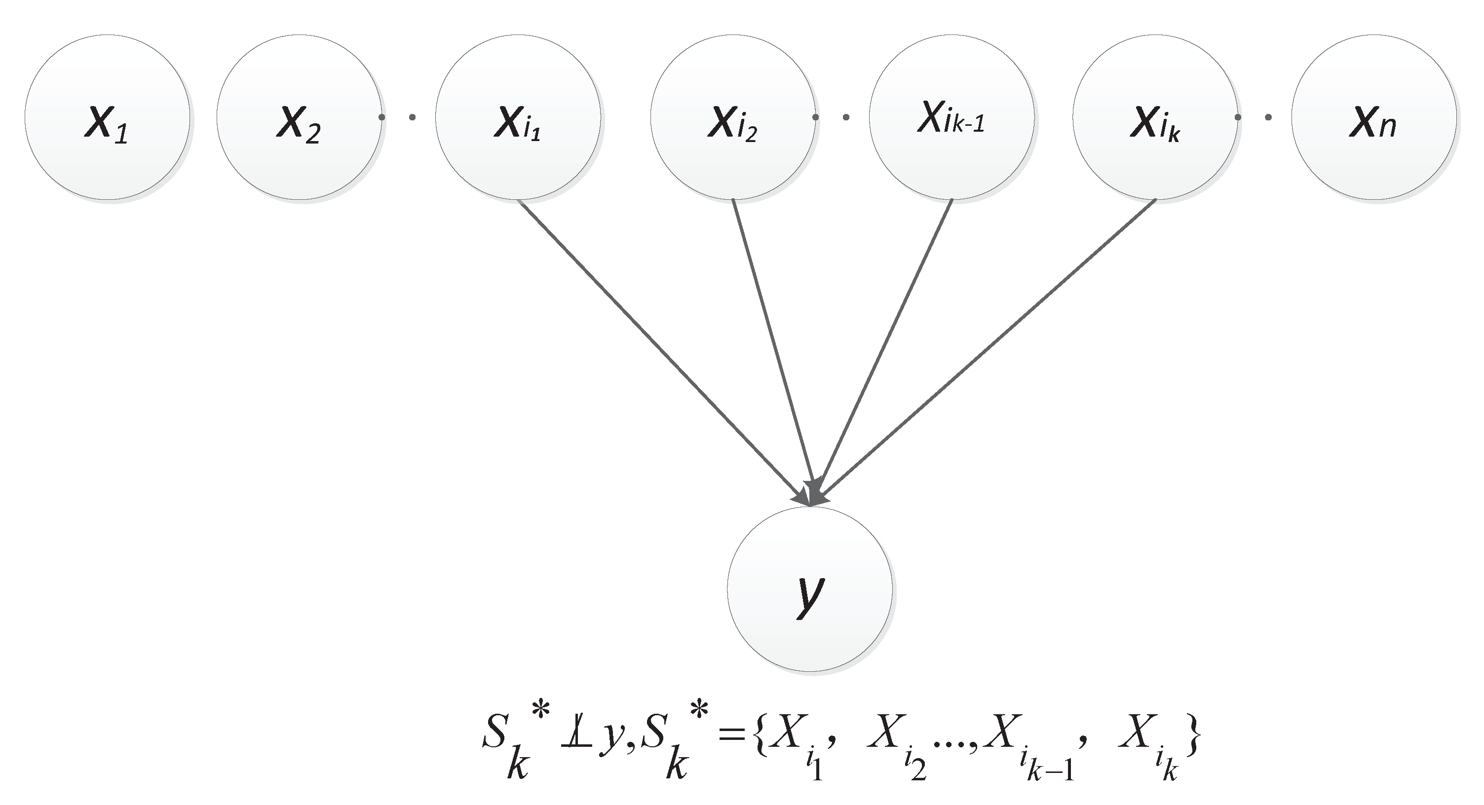
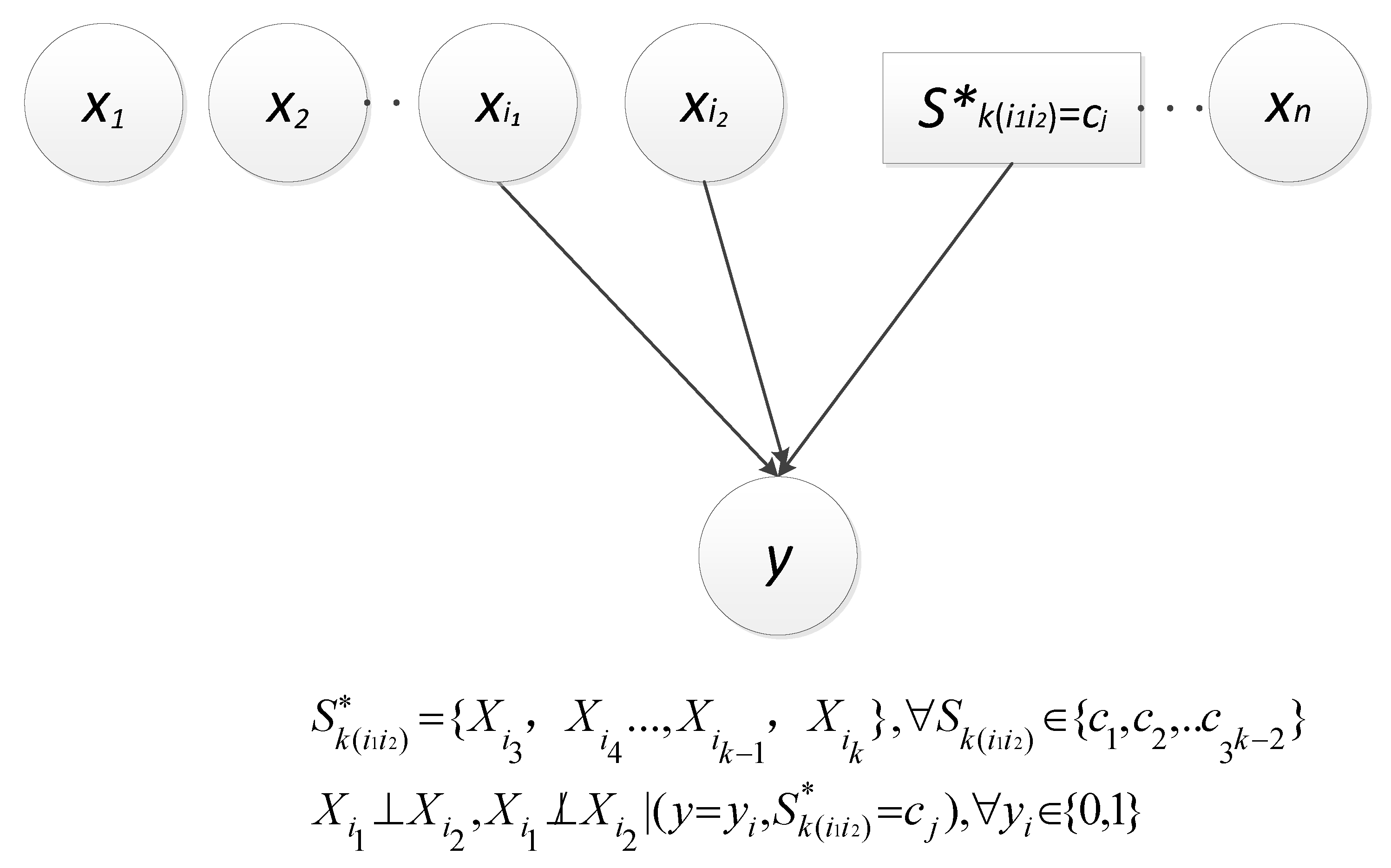
3.2. Causal Relationship

According to how the data are generated, the structural equation of the causal relationship between epistasis SNP combination and disease status can be modeled as [26]:
y = f ( s k ) + e y ,
where e y is the noise variable.
From the above equation, we can find that s k and e y are independent (denoted as s k e y ). In other words, among all s k S k , s k and e y have the lowest degree of dependency. However, it is unrealistic to measure the dependence degree of any s k and e y as the evaluation criterion for epistasis detection, because it requires too high a computational cost to obtain data generated by e y based on the regression method.
Thus, this paper herein let e y be the constant 0, i.e., y  f ( s k ) , which approximately introduces two kinds of dependencies as described in Figure 1 and Figure 2, respectively [25]. Obviously, the dependence between s and y is direct (denoted as s k y ); and the other is derived from the v-structure, i.e., x i 1 and x i 2 are dependent given a value of y and s k ( i 1 i 2 ) (denoted as x i 1 x i 2 | y = y i , s k ( i 1 i 2 ) = c j ). Let s k = { x i 1 , x i 2 , , x i k 1 , x i k } , s k ( i 1 i 2 ) represent s k \ { x i 1 , x i 2 } . In particular, the set s k ( i 1 i 2 ) is empty when k is equal to 2.

3.3. Scoring Criterion

These two kinds of dependencies described above inspire us to raise this scoring criterion, which integrates a widely used method of measuring statistical dependencies based on kernel functions (HSIC).
For s k S k , then, for x i 1 , x i 2 s k , given y = p ( p { 0 , 1 } ) and s k ( i 1 i 2 ) = q ( q { c 1 , c 2 , , c 3 k 2 } ), let D i 1 i 2 p q = ( X i 1 i 2 p q , Y i 1 i 2 p q ) be a slice of D on x i 1 , x i 2 under the constraint; m i 1 i 2 p q is the number of rows of the data slice ( m i 1 i 2 q = m i 1 i 2 0 q + m i 1 i 2 1 q ); HSIC ( X , Y ) is used to measure the degree of statistical dependence of two random variables (x and y) based on dataset (X, Y); the scoring criterion can be computed by the following Equations (2)–(6).
b i 1 i 2 q = m i 1 i 2 0 q m i 1 i 2 q HSIC ( X i 1 0 q , X i 2 0 q ) + m i 1 i 2 1 q m i 1 i 2 q HSIC ( X i 1 1 q , X i 2 1 q )
b q = i 1 i 2 , x i 1 , x i 2 s k ( m i 1 i 2 q i a i b , x i a , x i b s k m i a i b q b i 1 i 2 q )
m ¯ q = ( i a i b , x i a , x i b s k m i a i b q ) / c k 2
HSIC C R q = m m + m ¯ q HSIC ( X i 1 i 2 , i k , Y i 1 i 2 , i k ) + m ¯ q m + m ¯ q b q
HSIC C R ( X i 1 i 2 , i k , Y i 1 i 2 , i k : d a t a ) = q = 1 q = 3 k 2 HSIC C R q
To facilitate the reader’s understanding, we now define following notations:
1.
The value of b i 1 i 2 q is a linear weighted sum of HSIC ( X i 1 0 q , X i 2 0 q ) and HSIC ( X i 1 1 q , X i 2 1 q ) based on respective sample sizes;
2.
For all x i 1 , x i 2 s k , the value of b q is a linear weighted sum of all b i 1 i 2 q since there are c k 2 v-structures given s k ( i 1 i 2 ) = q ;
3.
The value of HSIC C R q is a linear weighted sum of HSIC ( X i 1 i 2 , i k , Y i 1 i 2 , i k ) and b q based on sample size of D i 1 i 2 , i k and average sample size of all D i a i b q , which is a component and basis of HSIC C R ;
4.
In particular, b i 1 i 2 q = b q as is HSIC C R q = HSIC C R when k = 2 ;
5.
For robustness purposes, let b i 1 i 2 q = 0 if and only if the denominator of the weighted factor term is 0, like b q ;
6.
The effort to calculate scoring criterion is reduced to calculate HSIC ( X i 1 i 2 , i k , Y i 1 i 2 , i k ) once, and is reduced up to C k 2 3 k 2 times to calculate the type of problem b i 1 i 2 q (fortunately, k { 2 , 3 , 4 , 5 } in practice).
Thus, our estimate of s k can eventually be obtained by solving the problem
m a x f ( D ) ( s k ) s k S k = HSIC C R ( X i 1 i 2 , i k , Y i 1 i 2 , i k )

3.4. Method for Measuring Statistical Dependence

3.4.1. HSIC

HSIC is a measuring statistical dependence criterion proposed by other authors [27,28] based on the eigenspectrum of covariance operators in reproducing kernel Hilbert spaces (RKHSs), denoted by HSIC P x y as follows:
HSIC P x y = E x , x , y , y k ( x , x ) l ( y , y ) +   E x , x k ( x , x ) E y , y l ( y , y )   2 E x , y [ E x [ k ( x , x ) ] E y [ l ( y , y ) ] ] ,
where k ( , ) and l ( , ) are two kernel functions.
Let X and Y be the separable sample spaces of random variables x and y, respectively, assuming that ( X , Γ ) and ( Y , Λ ) are furnished with probability measures p x , p y , respectively ( Γ being the Borel sets on X , and Λ the Borel sets on Y ); p x y is a joint measure over ( X × Y , Λ × Γ ) ; HSIC P x y 0 (the higher the degree of dependence of x and y, the greater the value) and HSIC P x y is zero if and only if x and y are independent.
In order to show that HSIC is a practical criterion for measuring independence or the degree of dependence given a finite number of observations, it consists of an empirical estimator with O ( m 1 ) expectation bias, denoted by HSIC D , formulated as follows:
HSIC D = ( m 1 ) 2 t r a c e ( K H L H ) ,
where D:= { ( x 1 , y 1 ) , , ( x m , y m ) } X × Y , K , H , L R m × m , K i , j : = k ( x i , x j ) , L i , j : = l ( y i , y j ) , H i , j : = δ i j m 1 .
An advantage of HSIC compared with other kernel-based independence criteria is that it can be computed in O ( m 2 ) time. However, such computational costs are too high as an integral part of the scoring criterion. Fortunately, the sample space of the disease status, SNP loci and k-order SNP combination is finite discrete. Thus, immediately below, we put forward an efficient HSIC calculation method for variables with a small sample, which can be approximately calculated in O ( m ) time. Thus, as k { 2 , 3 , 4 , 5 } , we can compute HSIC C R in O ( c k 2 × m ) O ( m ) time in practice.

3.4.2. Efficient Computation

Proposition 1
(Efficient computation). Let x and y be two random discrete variables with p and q states, respectively, where p 2 × q 2 < m , or p 2 × q 2 m . Then, we can compute t r a c e ( K H L H ) in O ( m ) time.
Proof. 
Let e be a column vector with a length of m, e = 1 . . 1 ,   L = l 1 t . . l m t , and I be an identity matrix with a size of m m ; we have H = I 1 m e e t and L H = L 1 m L e e t .
As 1 m L e = 1 m l 1 t e . . 1 m l m t e , which implies that each i-th element of 1 m L e is the mean of the corresponding row elements of L, we have L 1 m L e e t = l 1 t . . l m t 1 m l 1 ¯ . . 1 m l m ¯ e t , where each l i ¯ is the sum of the corresponding row elements of L.
Let L ¯ = 1 m l 1 ¯ . . 1 m l m ¯ e t be an m × m matrix ( L ¯ i j = 1 m l i ¯ ) and K ¯ = 1 m k 1 ¯ . . 1 m k m ¯ e t be an m × m matrix ( K ¯ i j = 1 m k i ¯ ); we have t r a c e ( K H L H ) = t r a c e ( ( K K ¯ ) ( L L ¯ ) ) .
Let P be an m × m row transformation matrix; we have t r a c e ( P K H P L H ) = t r a c e ( P ( K K ¯ ) P ( L L ¯ ) ) = t r a c e ( ( K K ¯ ) ( L L ¯ ) ) = t r a c e ( K H L H ) .
Thus, without a loss of generality, we can assume that: D= { ( c 1 , y i 1 ) , ( c 1 , y i 2 1 ) ,   ( c 2 , y i 2 ) , ( c 2 , y i 3 1 ) , ( c p , y i p ) , ( c p , y i m ) } , i.e., the number of observed instances of x with the value of c j (denoted as x t ( c j ) ) is i j + 1 i j ( i p + 1 = i m + 1 ); K can be viewed as a p × p partitioned matrix. Let K j l be the j × l th block having x t ( c j ) × x t ( c l ) elements, all having the same value ( k ( c j , c l ) ). Let K ^ = K K ¯ , where all elements in K ^ j l have the same value equal to k ( c j , c l ) n = 1 p x t ( c n ) × k ( c j , c n ) m (denoted as K ^ ( j , l ) ).
Let y x ( j , i ) be the number of observed instances with the value ( c i , d j ) ( 1 j q , d j is the j-th state of y); the definition of L ^ and L ¯ is similar to that of K ^ and K ¯ . We also view L ^ as a p × p partitioned matrix, where each L j l has the same number of rows and columns as K j l ; for p , 1 p m , 1 m l ¯ p = v = 1 q y t ( d v ) × k ( d h , d v ) m (denoted as l ¯ ( d h ) ), where y p = d h .
As t r a c e ( K ^ L ^ ) = i = 1 p j = 1 p < K ^ i j , ( L ^ j i ) T > (<.,.> denoted as inner product operator) and < K ^ i j , ( L ^ j i ) T > = K ^ ( i , j ) × u = 1 q y x ( u , j ) × v = 1 q ( y x ( v , i ) × ( l ( d u , d v ) l ¯ ( d u ) ) , we can obtain that the computational complexity of t r a c e ( K ^ L ^ ) is O ( p 2 q 2 ) .
As described above, we can know that the total computational complexity of x t , y t and y x is O ( m ) , and that those of K ¯ and L ¯ are O ( p 2 ) and O ( q 2 ) , respectively.
Hence, we have that the total computational complexity of HSIC is O ( m ) , where p 2 × q 2 < m , or p 2 × q 2 m .
The proof is complete.    □
In fact, the proof above gives the simplified process of efficient computation to HSIC . The detailed processes are shown in Algorithms 1–5. Algorithm 1 is the main process of the method, consisting of three functions:
  • (X, Y) is m observations of a tuple of x and y with p and q states, respectively;
  • k e r n e l s includes two kernel functions used to calculate K i , j and L i , j , the parameters of which are d e l t a ( 1 ) and d e l t a ( 2 ) , respectively;
  • G e t I n f o (see Algorithm 2) is used to calculate x t , y t and y x ;
  • For all 1 j , l p , K H (see Algorithm 3) is used to calculate K ^ ( j , l ) ;
  • T r a c e (see Algorithm 4) is used to calculate t r a c e ( K ^ L ^ ) ;
  • R o w A v e r a g e (see Algorithm 5) is used to calculate K ¯ and L ¯ .
Algorithm 1 Calculate v a l u e = HSIC ( X , Y , p , q , m , k e r n e l s , d e l t a s )
Require:
| X | = | Y | = m
1:
[ x t , y t , y x ] G e t I n f o ( X , Y , p , q , m )
2:
K ^ K H ( x t , p , k e r n e l s ( 1 ) , d e l t a s ( 1 ) , m )
3:
v a l u e T r a c e ( K ^ , y t , y x , p , q , k e r n e l s ( 2 ) , d e l t a s ( 2 ) , m )
Algorithm 2 Calculate [ x t , y t , y x ] = G e t I n f o ( X , Y , p , q , m )
  1:
x t z e r o s ( 1 , p )
  2:
y t z e r o s ( 1 , q )
  3:
y x z e r o s ( q , p )
  4:
c o l 1
  5:
while   c o l m  do
  6:
     s t x X ( c o l )
  7:
     s t y Y ( c o l )
  8:
     x t ( s t x ) x ( s t x ) + 1
  9:
     y t ( s t y ) y ( s t y ) + 1
10:
     y x ( s t y , s t x ) y x ( s t y , s t x ) + 1
11:
     c o l c o l + 1
12:
end while
Algorithm 3 Calculate K ^ = K H ( x t , p , k e r n e l , d e l t a , m )
  1:
K ¯ R o w A v e r a g e ( p , k , d e l t a , m , x t )
  2:
K ^ z e r o s ( p , p )
  3:
i 1
  4:
while   i p   do
  5:
     j 1
  6:
    while  j p  do
  7:
         K ^ ( i , j ) k e r n e l ( i , j , d e l t a ) K ¯ ( i )
  8:
         j j + 1
  9:
    end while
10:
     i i + 1
11:
end while
Algorithm 4 Calculate v a l u e = T r a c e ( K ^ , y t , y x , p , q , k e r n e l , d e l t a , m )
  1:
L ¯ R o w A v e r a g e ( q , k e r n e l , d e l t a , m , y t )
  2:
v a l u e 0
  3:
i 1
  4:
while   i p   do
  5:
     j 1
  6:
    while  j p  do
  7:
         u 1
  8:
         t 0
  9:
        while  u q  do
10:
            v 1
11:
            s 0
12:
           while  v q  do
13:
                s s + y x ( v , i ) × ( k e r n e l ( u , v , d e l t a ) L ¯ ( u ) )
14:
                v v + 1
15:
           end while
16:
            t t + y x ( u , j ) × s
17:
            u u + 1
18:
        end while
19:
         v a l u e v a l u e + K ^ ( i , j ) × t
20:
         j j + 1
21:
    end while
22:
     i i + 1
23:
end while
24:
v a l u e v a l u e / ( ( m 1 ) ( m 1 ) )
Algorithm 5 Calculate M ¯ = R o w A v e r a g e ( p , k e r n e l , d e l t a , m , y )
  1:
M ¯ z e r o s ( 1 , p )
  2:
i 1
  3:
while  i p  do
  4:
     j 1
  5:
    while  j p  do
  6:
         M ¯ ( i ) M ¯ ( i ) + y ( j ) k e r e n l ( i , j , d e l t a )
  7:
         j j + 1
  8:
    end while
  9:
     M ¯ ( i ) M ¯ ( i ) / m
10:
     i i + 1
11:
end while

4. Experiments

We employed representation of the data in a matrix X i j p q { 0 , 1 , 2 } m i j p q × 1 to calculate HSIC ( X i 1 p q , X i 2 p q ) by using a Gaussian kernel ( σ 2 = 0.1 ). In addition, we mapped X i 1 i 2 , i k { 0 , 1 , 2 } m × k onto X i 1 i 2 , i k { 0 , 1 } m × 3 k to compute HSIC ( X i 1 i 2 , i k , Y i 1 i 2 , i k ) by also using a Gaussian kernel ( σ 2 = 1 ), i.e., 0 ( 1 , 0 , 0 ) , 1 ( 0 , 1 , 0 ) and 2 ( 0 , 0 , 1 ) . The advantages and disadvantages of the two representations have been explained by the other authors [29].

4.1. Evaluation Criterion

The evaluation criterion that we adopted in the experiments is by [9]:
P o w e r = S T ,
where S is the number of found disease-causing SNP combinations (the epistasis SNPs score the highest) and T is the number of datasets. Each dataset includes one disease-causing SNP combination. P o w e r is a measure of the accuracies of scoring criteria from genome data.

4.2. Simulated Datasets

For any data set, the worst-case scenario for checking the correctness of the scoring criteria is extensive testing of all SNP combinations. It is too computationally expensive for k = 4 and k = 5 cases. Therefore, tests were only conducted for k = 2 and k = 3.

4.2.1. Disease Models with k = 2

For k = 2, we used thirty-five disease models without marginal effects (DNME1–35) and six disease models with marginal effects (DME1–6). The models were designed based on interaction structures with different diseases, MAFs, prevalence (p) and h (the parameter settings are described in the supplementary files). Each data set contains 1000 SNPs and includes pairs of interacting SNPs (M0P0 and M1P1) generated according to the disease model setting, while other SNPs are generated using MAFs uniformly selected in [0.05, 0.5). For each model, we generated two simulated 100 data sets using the software GAMETES2.1 [30] with sample sizes of 400 (200 controls and 200 cases) and with sample sizes of 800 (400 control and 400 cases) [31].

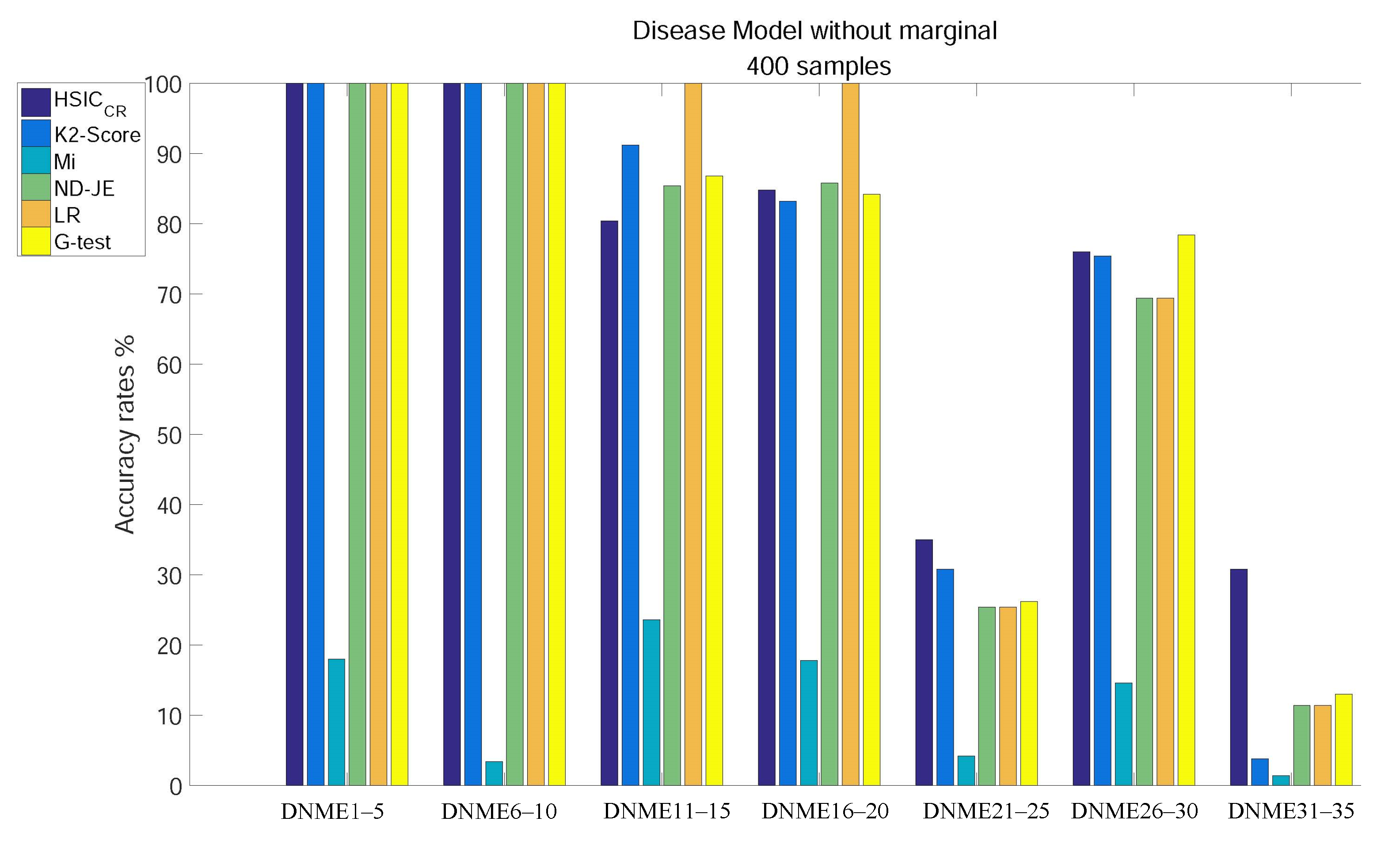
Disease Models without Marginal Effects

We divided all DNMEs into seven subgroups for analysis according to the different combined values of h and MAF (DNME1–5 MAF = 0.2, h = 0.2; DNME6–10 MAF = 0.4, h = 0.2; DNME11–15 MAF = 0.2, h = 0.1; DNME16–20 MAF = 0.4, h = 0.1; DNME21–25 MAF = 0.2, h = 0.05; DNME25–30 MAF = 0.4, h = 0.05; DNME1–5 MAF = 0.2, h = 0.025).
The analysis results of subgroups of DNME1–35, each of which has 400 samples, are shown in Figure 3:
  • Except for Mi, using tests on DNME1–10, the accuracy of all scoring criteria is close to 100%;
  • All criteria are not very accurate using tests on DNME21–25 and DNME31–35;
  • Mi has an extremely poor accuracy on all subgroup tests;
  • LR has the highest accuracy using tests on DNME11–15 and DNME16–20, close to 100%, but is only a little more accurate than Mi on DNME21–25, DNME26–30 and DNME31–35 tests;
  • The accuracy rates of both ND-JE and G-test rank in the middle overall, but G-test has the highest accuracy on the DNME26–30 test;
  • The accuracy rate of K2-Score ranks second on DNME11–15 and DNME21–25 tests, third on the DNME26–30 test and slightly worse than ND-JE, HS C R and G-test on the DNME16–20 test, but is only a little more accurate than Mi on the most difficult model (DNME31–35) test;
  • HSIC C R has the highest accuracy on the two most difficult model subgroup (DNME21–25 and DNME31–35) tests, especially on DNME31–35, where the accuracy is much higher than other criteria, and the overall accuracy on other model subgroups tests is similar to the other four criteria.
When the size of samples increased from 400 to 800, the accuracy of all criteria was greatly improved. The analysis results of subgroups of DNME1–35, each of which has 800 samples, are shown in Figure 4:
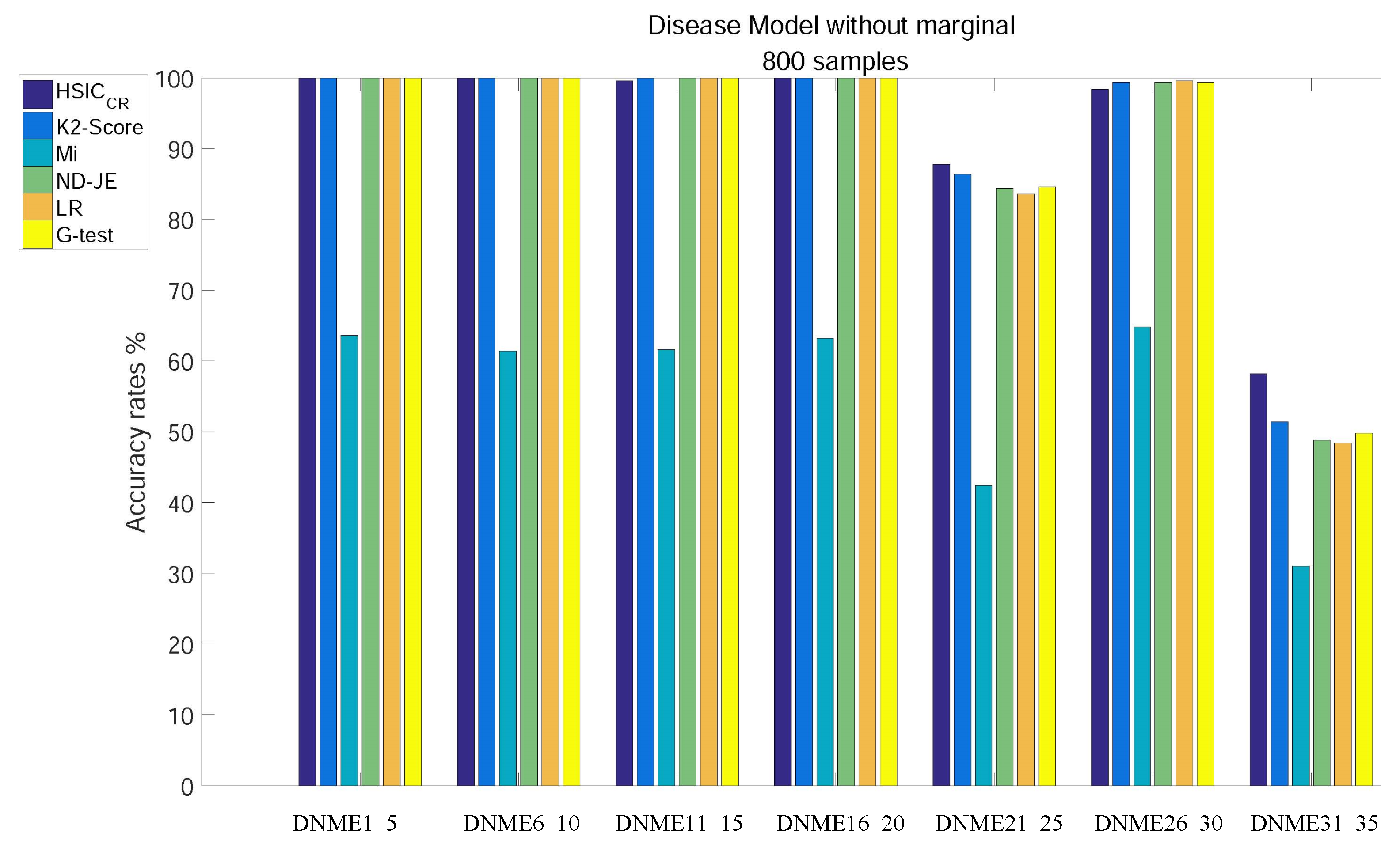
  • Except for Mi, the accuracy of all criteria is close to 100% excluding tests on the two most difficult model subgroups (DNME21–25 and DNME31–35);
  • Although the accuracy rate of Mi can be significantly improved with the increase in the size of samples, it is still relatively poor overall;
  • With the number of samples increasing, there is still no change in the overall ranking, but the accuracy of the K2-Score on the DNME31–35 test rises to second;
  • HSIC C R has the highest accuracy on the two most difficult model subgroup tests.
Table 1 reveals the total average accuracy. From Table 1, we can find that Mi has a poor average accuracy; HSIC C R has the best average accuracy regardless of the model’s sample scale of 400 or 800; although HSIC C R is only slightly higher than the other four criteria on the total average accuracy, and the average accuracy on the most difficult model subgroup test is much better than other criteria.

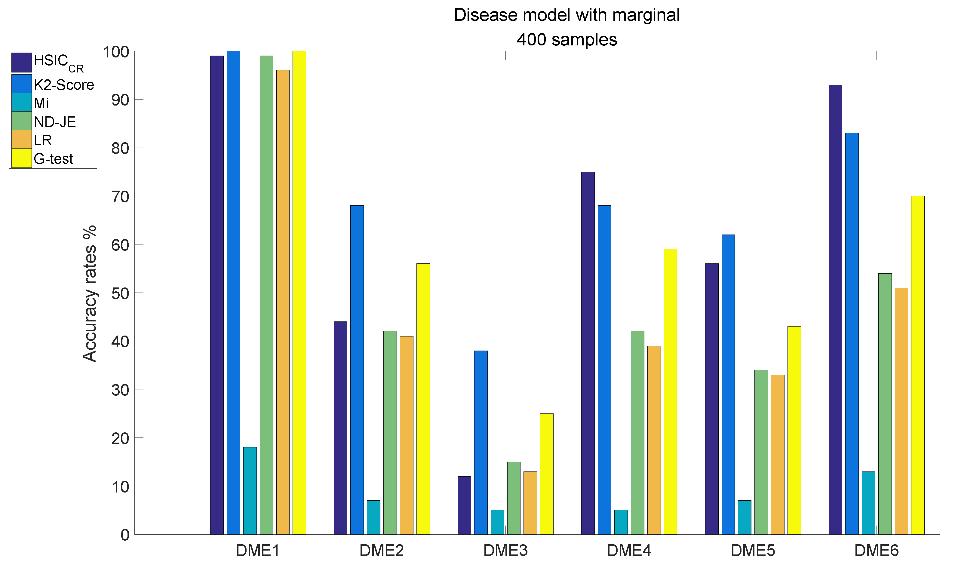
Disease Models with Marginal Effects

We tested six DMEs for analysis according to MAF = 0.1 and the different combined values of heritability and prevalence (DME1 h = 0.031 and p = 0.050; DME2 h = 0.014 and p = 0.050; DME3 h = 0.01 and p = 0.050; DME4 h = 0.016 and p = 0.046; DME5 h = 0.009 and p = 0.026; DME6 h = 0.008 and p = 0.017).
The analysis results of DME1–6, each of which has 400 samples, are shown in Figure 5:
  • The accuracy of all scoring criteria is close to 100% tested on DME1, except for Mi;
  • Mi has extremely poor accuracy on all six models tests;
  • Except for Mi, the accuracy rate of LR is worse than the other four criteria on DME2–6 tests, except that the accuracy on the DME3 test is nearly the same as that of HSIC C R ;
  • The accuracy rate of ND-JE ranks third on DME1 and DME3 tests, and fourth on the other four models tests;
  • The accuracy rate of G-test ranks first on the DME1 test, second on DME2 and DME3 tests and third on the other four models tests;
  • HSIC C R has the highest accuracy rate on DME4 and DME6 tests, its accuracy rate on the DME5 test is slightly worse than LR and the accuracy rate on DME1–2 tests ranks third, whereas the accuracy rate on the DME3 test is a little better than Mi;
  • K2-Score has the highest accuracy rate on DME1–3 and DME5 tests, its accuracy rate on DME4 and DME6 tests ranks second and it significantly outperforms the others on the most difficult model (DME3) test (although its accuracy rate in DME3 is below 50%).
When the size of samples increased from 400 to 800, the accuracy of all criteria was greatly improved. The analysis results of DME1–6, each of which has 800 samples, are shown in Figure 6:
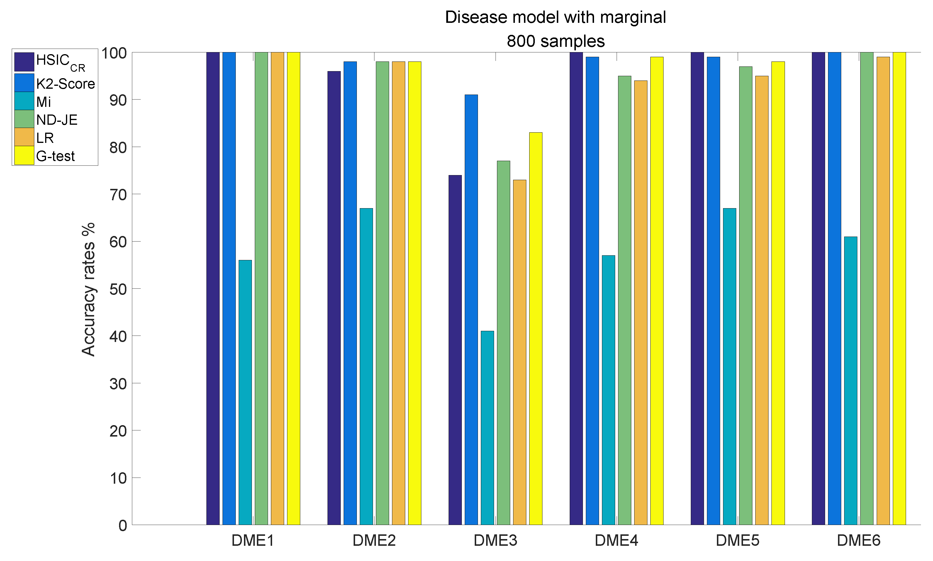
  • Although the accuracy of Mi can be significantly improved with the increase in the size of samples, it is still relatively poor overall;
  • The accuracy rates of the other five scoring criteria all exceed 95% tested by the models, except on DME3;
  • K2-Score has the highest accuracy rate on the most difficult model test (over 90%), the accuracy rate of G-test ranks second (over 80 %) and the accuracy rates of ND-JE, HSIC C R and LR are not good enough, at just over 70 % .
Table 2 reveals the total average accuracy. From Table 2, we can find that Mi has a poor average accuracy; the K2-Score has the best average accuracy rate regardless of the model’s sample scale of 400 or 800, where the main reason is that its accuracy rate on the DME3 test is much better than the other five scoring criteria; although the average accuracy of HSIC C R tested on DME3 is not good enough, it ranks second in the overall average accuracy rate.

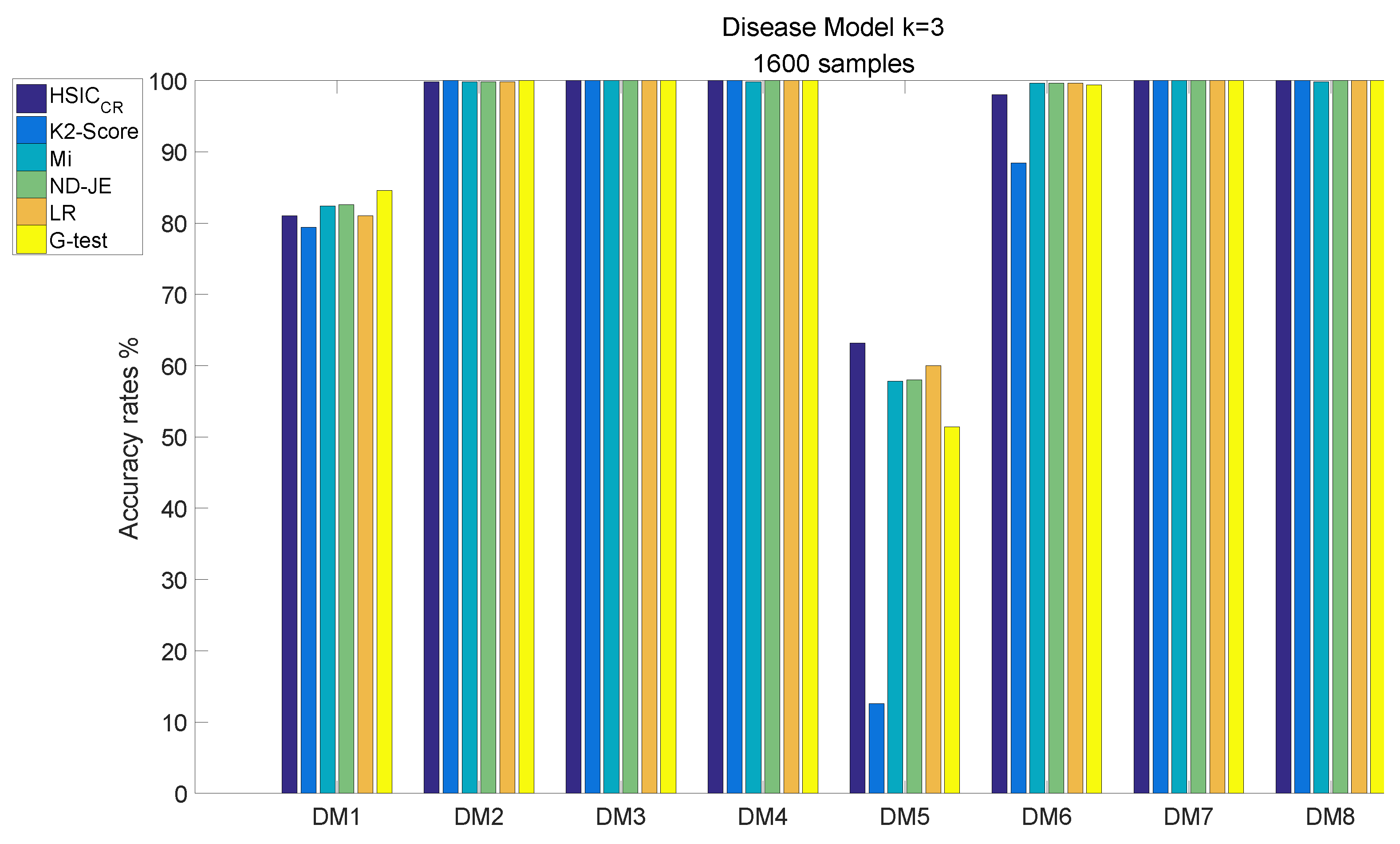
4.2.2. Disease Models with k = 3

For k = 3 , the data sets are generated by eight third-order epistasis pathogenic models (DM1–8), which are modeled by GAMETES2.1 according to the combinations of different MAFs ([0.2, 0.4]) and different heritability ([0.025, 0.05, 0.1, 0.2]) (DM1 MAF = 0.2, h = 0.025; DM2 MAF = 0.2, h = 0.05; DM3 MAF = 0.2, h = 0.1; DM4 MAF = 0.2, h = 0.2; DM5 MAF = 0.4, h = 0.025; DM6 MAF = 0.4, h = 0.05; DM7 MAF = 0.4, h = 0.1; DM8 MAF = 0.4 h = 0.2). The ♯quantiles of each combination is five. Every quantile of each pathogenic model corresponds to 100 simulated data files. Each file contains 100 SNPs and 1600 samples (800 normal, 800 diseased), and includes three interacting SNPs (M0P0, M1P1 and M2P2) generated according to the disease model settings, while other SNPs were generated using MAFs uniformly selected in [0.05, 0.5]. Therefore, the total number of the data sets is 4000 [6]. Detailed parameter settings are described in the supplementary file.
The analysis results of DM1–8, each of which has 1600 samples, are shown in Figure 7:
  • The accuracy of all scoring criteria is close to 100% tested on DM2, DM3–4 and DM7–8;
  • The accuracy of all scoring criteria is close to 80% on the DM1 test;
  • The K2-Score has a poor accuracy rate on the most difficult model (DM5) test, whose accuracy is just close to 10 % ;
  • The accuracy rates of the scoring criteria on the DM6 test are good enough, and the accuracy rates of the scoring criteria are close to 100%, except the K2-Score;
  • HSIC C R has the highest accuracy rate on the DM5 test, and its accuracy rate is the only one that exceeds 60% among all scoring criteria.
Table 3 reveals the total average accuracy. From Table 3, we can find that the K2-Score has a poor average accuracy on the most difficult model test; the total average accuracy rates for all scoring criteria are good enough, with all criteria except the K2-Score achieving over 90% accuracy. Although HSIC has the best total average accuracy, its accuracy is not significantly better than other four criteria; however, tested on the most difficult model, the accuracy rate of HSIC C R outperforms LR by 3.2%, and significantly outperforms the other four criteria, especially the K2-Score.

4.2.3. The Running Time Analysis

To demonstrate that our proposed method can be used as a lightweight scoring criterion, we proved in the previous section that its time complexity is O ( m ) . Furthermore, we calculated the average running time per dataset (unit in seconds) for the two-order with a sample size of 800 and the three-order in the simulation experiments, and we found that the average running time per dataset of our proposed method is between the other five lightweight methods (see Table 4). This further demonstrates the applicability of our proposed method as a lightweight scoring criterion.
In the experiment, all scoring criteria were implemented based on Matlab, and all tests were run on the environment of Windows 10 64 desktop computer with 11th Gen Intel(R) Core(TM) i7-1165G7 @ 2.80 GHz, and 16.0 GB memory.

4.3. Case Study: A Real Chronic Dialysis Data

A real data set of 193 cases and 704 controls was selected from the mitochondrial D-loop region of chronic dialysis patients who were observed in a study by other authors [32]. The genotypes and locations of 77 SNPs are presented in Table 5 [33].
The 77 SNPs contained in the subset of the chronic dialysis data set were used in the case study, which aims to give our readers more specificity regarding our proposed scoring criterion. First, for this dataset, we performed a full-space two-order SNP combination detection, meaning that the HSIC C R values were evaluated for 2926 ( C 77 2 ) possible combinations. Then, we selected the top ten HISC C R -valued combinations as candidate two-order epistasis SNP combinations to be raised for medical researchers, and the 10 candidate combinations are presented in Table 6.

5. Conclusions

In this paper, we verified with rigorous mathematical proof that HSIC C R can be computed in O ( m ) time. Moreover, we compared HSIC C R with five representative scoring criteria for 49 simulation disease models. The experimental results show that: Mi has a poor accuracy on two-order disease models; the K2-Score has a poor accuracy on three-order difficult disease models; the accuracy rates of LR are not good enough on two-order disease models tests; HSIC C R , G-test and ND-JE have a high accuracy on all three classes of disease models tests; the accuracy rates of HSIC C R rank first on two-order disease models without marginal effects tests and three-order disease model tests, and rank second on two-order disease models with marginal effects tests, although its advantage is not significant.
The advantages of HSIC C R are: the methodology used is different from other scoring criteria, which makes it more complementary to other scoring criteria; it has a high accuracy on most disease models.
In the future, we will further investigate proposing efficient SIO algorithms to solve this problem by combining HSIC C R and other effective lightweight criteria that already exist as weighted single or multi-objective functions. In addition, we will work with several local medical research institutions to use their real disease case-control study data to mine for disease-related SNP combinations by using our proposed approach. This will ultimately provide new guidance for drug development in complex diseases.

Supplementary Materials

The following supporting information can be downloaded at: https://www.mdpi.com/article/10.3390/math10214134/s1, Table S1: Model with marginal effects when k = 2; Table S2: Models 1 to 10 without marginal effects when k = 2; Table S3: Models 11 to 20 without marginal effects when k = 2; Table S4: Models 21 to 30 without marginal effects when k = 2; Table S5: Models 31 to 35 without marginal effects when k = 2.

Author Contributions

Conceptualization, J.Z. (Junxi Zheng); data curation, J.Z. (Junxi Zheng) and J.Z. (Jiaxian Zhu); formal analysis, J.Z. (Juan Zeng), J.Z. (Jiaxian Zhu) and F.W.; funding acquisition, J.Z. (Junxi Zheng); investigation, G.L. and F.W.; methodology, J.Z. (Junxi Zheng); project administration, D.T. and X.W.; supervision, D.T. and X.W.; validation, J.Z. (Junxi Zheng) and J.Z. (Juan Zeng); visualization, G.L.; writing—original draft, J.Z. (Junxi Zheng) and X.W. All authors have read and agreed to the published version of the manuscript.

Funding

This work was supported by the Guangdong provincial medical research foundation of China (No. A2022531), the national natural science foundation of China (No. 61976239), and the natural science foundation of Guangdong province, China (No. 2020A1515010783).

Data Availability Statement

The data that support the findings of this study can be acquired from the corresponding author.

Conflicts of Interest

No potential conflict of interest was reported by the authors.

Abbreviations

The following abbreviations are used in this manuscript:
SNPsingle-nucleotide polymorphism
GWASgenome-wide association analysis

References

  1. Carlson, C.S.; Eberle, M.A.; Kruglyak, L.; Nickerson, D.A. Mapping complex disease loci in whole-genome association studies. Nature 2004, 429, 446–452. [Google Scholar] [CrossRef] [PubMed]
  2. Wei, W.H.; Hemani, G.; Haley, C.S. Detecting epistasis in human complex traits. Nat. Rev. Genet. 2014, 15, 722–733. [Google Scholar] [CrossRef]
  3. Guo, X.; Meng, Y.; Yu, N.; Pan, Y. Cloud computing for detecting high-order genome-wide epistatic interaction via dynamic clustering. BMC Bioinform. 2014, 15, 102. [Google Scholar] [CrossRef] [Green Version]
  4. Guo, X.; Zhang, J.; Cai, Z.; Du, D.Z.; Pan, Y. Searching genome-wide multi-locus associations for multiple diseases based on bayesian inference. IEEE/ACM Trans. Comput. Biol. Bioinform. 2016, 14, 600–610. [Google Scholar] [CrossRef]
  5. Gyenesei, A.; Moody, J.; Semple, C.A.; Haley, C.S.; Wei, W.H. High-throughput analysis of epistasis in genome-wide association studies with BiForce. Bioinformatics 2012, 28, 1957–1964. [Google Scholar] [CrossRef] [Green Version]
  6. Liyan, S. The Research on Epistasis Detection Algorithm in Genome-wide Association Study. Ph.D. Thesis, Jilin University, Changchun, China, 2020. [Google Scholar]
  7. Ritchie, M.D.; Hahn, L.W.; Roodi, N.; Bailey, L.R.; Dupont, W.D.; Parl, F.F.; Moore, J.H. Multifactor-dimensionality reduction reveals high-order interactions among estrogen-metabolism genes in sporadic breast cancer. Am. J. Hum. Genet. 2001, 69, 138–147. [Google Scholar] [CrossRef] [PubMed] [Green Version]
  8. Wang, X.; Cao, X.; Feng, Y.; Guo, M.; Yu, G.; Wang, J. ELSSI: Parallel SNP–SNP interactions detection by ensemble multi-type detectors. Brief. Bioinform. 2022, 23, bbac213. [Google Scholar] [CrossRef] [PubMed]
  9. Tuo, S.; Liu, H.; Chen, H. Multipopulation harmony search algorithm for the detection of high-order SNP interactions. Bioinformatics 2020, 36, 4389–4398. [Google Scholar] [CrossRef]
  10. Sun, Y.; Shang, J.; Liu, J.X.; Li, S.; Zheng, C.H. epiACO—A method for identifying epistasis based on ant Colony optimization algorithm. BioData Min. 2017, 10, 23. [Google Scholar] [CrossRef] [Green Version]
  11. Tuo, S.; Zhang, J.; Yuan, X.; He, Z.; Liu, Y.; Liu, Z. Niche harmony search algorithm for detecting complex disease associated high-order SNP combinations. Sci. Rep. 2017, 7, 11529. [Google Scholar] [CrossRef]
  12. Aflakparast, M.; Salimi, H.; Gerami, A.; Dubé, M.; Visweswaran, S.; Masoudi-Nejad, A. Cuckoo search epistasis: A new method for exploring significant genetic interactions. Heredity 2014, 112, 666–674. [Google Scholar] [CrossRef] [PubMed] [Green Version]
  13. Jing, P.J.; Shen, H.B. MACOED: A multi-objective ant colony optimization algorithm for SNP epistasis detection in genome-wide association studies. Bioinformatics 2015, 31, 634–641. [Google Scholar] [CrossRef] [PubMed] [Green Version]
  14. Cheng, R.; Jin, Y.; Olhofer, M.; Sendhoff, B. A reference vector guided evolutionary algorithm for many-objective optimization. IEEE Trans. Evol. Comput. 2016, 20, 773–791. [Google Scholar] [CrossRef] [Green Version]
  15. Shouheng, T.; Hong, H. DEaf-MOPS/D: An improved differential evolution algorithm for solving complex multi-objective portfolio selection problems based on decomposition. Econ. Comput. Econ. Cybernet. Stud. Res. 2019, 53, 151–167. [Google Scholar]
  16. Verzilli, C.J.; Stallard, N.; Whittaker, J.C. Bayesian graphical models for genomewide association studies. Am. J. Hum. Genet. 2006, 79, 100–112. [Google Scholar] [CrossRef] [Green Version]
  17. Cooper, G.F.; Herskovits, E. A Bayesian method for the induction of probabilistic networks from data. Mach. Learn. 1992, 9, 309–347. [Google Scholar] [CrossRef] [Green Version]
  18. Jiang, X.; Neapolitan, R.E.; Barmada, M.M.; Visweswaran, S. Learning genetic epistasis using Bayesian network scoring criteria. BMC Bioinform. 2011, 12, 89. [Google Scholar] [CrossRef] [Green Version]
  19. Zhang, Y.; Liu, J.S. Bayesian inference of epistatic interactions in case-control studies. Nat. Genet. 2007, 39, 1167–1173. [Google Scholar] [CrossRef]
  20. Paninski, L. Estimation of entropy and mutual information. Neural Comput. 2003, 15, 1191–1253. [Google Scholar] [CrossRef] [Green Version]
  21. Lin, J. Divergence measures based on the Shannon entropy. IEEE Trans. Inf. Theory 1991, 37, 145–151. [Google Scholar] [CrossRef] [Green Version]
  22. Bush, W.S.; Edwards, T.L.; Dudek, S.M.; McKinney, B.A.; Ritchie, M.D. Alternative contingency table measures improve the power and detection of multifactor dimensionality reduction. BMC Bioinform. 2008, 9, 238. [Google Scholar] [CrossRef] [PubMed]
  23. Neyman, J.; Pearson, E.S. On the use and interpretation of certain test criteria for purposes of statistical inference: Part I. Biometrika 1928, 20A, 175–240. [Google Scholar]
  24. Stamatis, D.H. Essential Statistical Concepts for the Quality Professional; CRC Press: Boca Raton, FL, USA, 2012. [Google Scholar]
  25. Pearl, J. Models, Reasoning and Inference; Cambridge University Press: Cambridge, UK, 2000; Volume 19. [Google Scholar]
  26. Schaid, D.J. Genomic similarity and kernel methods I: Advancements by building on mathematical and statistical foundations. Hum. Hered. 2010, 70, 109–131. [Google Scholar] [CrossRef]
  27. Gretton, A.; Bousquet, O.; Smola, A.; Schölkopf, B. Measuring statistical dependence with Hilbert-Schmidt norms. In Proceedings of the International Conference on Algorithmic Learning Theory, Singapore, 8–11 October 2005; Springer: Berlin/Heidelberg, Germany, 2005; pp. 63–77. [Google Scholar]
  28. Gretton, A.; Fukumizu, K.; Teo, C.; Song, L.; Schölkopf, B.; Smola, A. A kernel statistical test of independence. Adv. Neural Inf. Process. Syst. 2007, 20, 585–592. [Google Scholar]
  29. Kodama, K.; Saigo, H. KDSNP: A kernel-based approach to detecting high-order SNP interactions. J. Bioinform. Comput. Biol. 2016, 14, 1644003. [Google Scholar] [CrossRef] [Green Version]
  30. Urbanowicz, R.J.; Kiralis, J.; Sinnott-Armstrong, N.A.; Heberling, T.; Fisher, J.M.; Moore, J.H. GAMETES: A fast, direct algorithm for generating pure, strict, epistatic models with random architectures. BioData Min. 2012, 5, 16. [Google Scholar] [CrossRef] [PubMed] [Green Version]
  31. Yang, C.H.; Chuang, L.Y.; Lin, Y.D. Multiobjective multifactor dimensionality reduction to detect SNP–SNP interactions. Bioinformatics 2018, 34, 2228–2236. [Google Scholar] [CrossRef] [Green Version]
  32. Chen, J.B.; Yang, Y.H.; Lee, W.C.; Liou, C.W.; Lin, T.K.; Chung, Y.H.; Chuang, L.Y.; Yang, C.H.; Chang, H.W. Sequence-based polymorphisms in the mitochondrial D-loop and potential SNP predictors for chronic dialysis. PLoS ONE 2012, 7, e41125. [Google Scholar] [CrossRef] [Green Version]
  33. Yang, C.H.; Kao, Y.K.; Chuang, L.Y.; Lin, Y.D. Catfish Taguchi-based binary differential evolution algorithm for analyzing single nucleotide polymorphism interactions in chronic dialysis. IEEE Trans. Nanobiosci. 2018, 17, 291–299. [Google Scholar] [CrossRef]
Figure 1. Direct dependence.
Mathematics 10 04134 g001
Figure 2. V-structure-related dependence.
Mathematics 10 04134 g002
Figure 3. Disease model without marginal effects, with 400 samples and with k = 2 .
Mathematics 10 04134 g003
Figure 4. Disease model without marginal effects, with 800 samples and with k = 2 .
Mathematics 10 04134 g004
Figure 5. Disease model with marginal effects, with 400 samples and k = 2 .
Mathematics 10 04134 g005
Figure 6. Disease model with marginal effects, with 800 samples and k = 2 .
Mathematics 10 04134 g006
Figure 7. Disease model with 1600 samples and k = 3 .
Mathematics 10 04134 g007
Table 1. The number of times, out of 3500 data sets generated by 35 models without marginal effects, where k = 2 , that each scoring criterion identified epistasis SNPs of snp1000 for sample sizes of 400 and 800. The fourth column gives the total accuracy over all sample sizes. The last column gives the accuracy over all sample sizes in the most difficult subgroup models. The scoring criteria are listed in descending order of total accuracy.
Scoring Criterion400 Samples800 SamplesTotal (%)DNME31–35 (%)
HSIC C R 253532205755 (82.2%)445 (44.5%)
K2-Score247931865665 (80.9%)336 (33.6%)
G-test244331695612 (80.2%)314 (31.4%)
ND-JE244031635603 (80.0%)301 (30.1%)
LR243731585595 (79.9%)297 (29.7%)
Mi49419712465 (35.2%)192 (19.2%)
Table 2. The number of times, out of 600 data sets generated by six models with marginal effects, where k = 2 , that each scoring criterion identified epistasis SNPs of snp1000 for sample sizes of 400 and 800. The fourth column gives the total accuracy over all sample sizes. The last column gives the accuracy over all sample sizes in the most difficult model. The scoring criteria are listed in descending order of total accuracy.
Scoring Criterion400 Samples800 SamplesTotal (%)DME3 (%)
K2-Score4195861005 (83.8%)159 (79.5%)
HSIC C R 379570949 (79.1%)86 (43%)
G-test353578931 (77.6%)108 (54%)
ND-JE286567853 (71.1%)92 (46%)
LR273559832 (69.3%)86 (43%)
Mi55349404 (33.7%)48 (24%)
Table 3. The number of times, out of 4000 data sets generated by eight models, where k = 3 , that each scoring criterion identified epistasis SNPs of snp100 for 1600 samples. The second column gives the total accuracy over a sample size of 1600. The last column gives the accuracy over a sample size of 1600 in the most difficult model. The scoring criteria are listed in descending order of total accuracy.
Scoring CriterionTotal (%)DM5 (%)
HSIC C R 3710 (92.8%)316 (63.2%)
LR3702 (92.6%)300 (60%)
ND-JE3700 (92.5%)290 (58%)
Mi3696 (92.4%)289 (57.8%)
G-test3677 (91.9%)257 (51.4%)
K2-Score3402 (85.1%)63 (12.6%)
Table 4. Average running time (s) for the six scoring criteria per dataset for both the two-order tests and the three-order tests in the simulation experiments.
Scoring Criterion2-Order (s)3-Order (s)
HSIC C R 120.242680.3045
LR77.305555.4438
ND-JE134.92276.5377
Mi78.355.6138
G-test77.658956.5221
K2-Score125.065581.4237
Table 5. Positions of chronic dialysis-associated 77 SNPS in mitochondrial d-loop region. a Left and right letters are major and minor genotypes, respectively. The number is the SNP position in the mitochondrial D-loop region.
SNP D-Loop Position
1∼5A16051G a T16086CT16092MT16093CC16108T
6∼10C16111TT16126CG16129AT16136CT16140C
11∼15G16145AC16148TT16157CA16162GA16164G
16∼20C16167TT16172CT16209CT16217CC16218T
21∼25T16223CA16227GC16234TA16235GT16243M
26∼30C16248TT16249CC16256TC16257WC16260T
31∼35C16261TC16266DA16272GG16274AC16278T
36∼40C16290TC16291TC16295TC16297TC16298T
41∼45C16304TA16309GT16311CA16316GG16319A
46∼50T16324CC16327TA16335GC16355TT16356C
51∼55T16357CT16362CG16390AA16399GA16463G
56∼60C16519TA93GG103AT146MC150T
61∼65C151TT152CA153GG185AA189G
66∼70C194TT195CT199CA200GT204C
71∼75G207AA210GT217CA234GA235G
76∼77T317CC461T
Table 6. The top ten highest HISC C R -valued two-order SNPs were used as ten candidate combinations.
RankCombinationHSIC CR
141,   210.035922
252,   210.033105
341,   170.019069
456,   210.018961
568,   390.018545
621,   190.017254
760,   210.014506
817,   80.011645
917,   140.0097405
1075,   360.0095467
Publisher’s Note: MDPI stays neutral with regard to jurisdictional claims in published maps and institutional affiliations.

