A Metaheuristic Optimization Approach to Solve Inverse Kinematics of Mobile Dual-Arm Robots

Abstract

This work presents an approach to solving the inverse kinematics of mobile dual-arm robots based on metaheuristic optimization algorithms. First, a kinematic analysis of a mobile dual-arm robot is presented. Second, an objective function is formulated based on the forward kinematics equations. The kinematic analysis does not require using any Jacobian matrix nor its estimation; for this reason, the proposed approach does not suffer from singularities, which is a common problem with conventional inverse kinematics algorithms. Moreover, the proposed method solves cooperative manipulation tasks, especially in the case of coordinated manipulation. Simulation and real-world experiments were performed to verify the proposal’s effectiveness under coordinated inverse kinematics and trajectory tracking tasks. The experimental setup considered a mobile dual-arm system based on the KUKA^® Youbot^® robot. The solution of the inverse kinematics showed precise and accurate results. Although the proposed approach focuses on coordinated manipulation, it can be implemented to solve non-coordinated tasks.

1. Introduction

The inverse kinematics of robot manipulators is an essential task to solve problems such as trajectory tracking, visual control, grasping, etc. Although robotic manipulators have many qualities, they have the drawback that they are fixed to a specific location with a limited workspace. To increase the manipulator’s workspace, the robot is attached to a mobile platform. These robots are called mobile manipulators and are used to solve robot manipulation tasks and mobile navigation simultaneously. However, the total degrees of freedom (DOFs) of both the manipulator and the platform give, as a result, a redundant robot [1]. The inverse kinematics for redundant robots is challenging to solve because redundancy admits several joint configurations to reach the same end-effector pose.

On the other hand, these robots allow us to solve complex tasks where just one manipulator is not enough, such as human-like tasks in domestic and industrial environments. It is important to remark that cooperative manipulation is a crucial task to solve for multiple manipulators that work together. Dual-arm systems are commonly used to deal with cooperative manipulation.

In general, there are non-coordinated manipulation and coordinated manipulation [2]. In non-coordinated manipulation, the robots perform different tasks, and the inverse kinematics can be solved independently. Robots interact with each other in coordinated manipulation, and the kinematics must be analyzed carefully to perform a task. Dual-arm systems increase the manipulation capabilities with greater accessibility. However, these systems are still fixed to a specific localization with a limited workspace. The dual-arm system is attached to a mobile platform to handle this inconvenience. The cooperative manipulation of mobile dual-arm systems is more challenging because the two manipulators interact on the same mobile platform. This inconvenience complicates the inverse kinematics, even in the case of non-coordinated manipulation.

Additionally, mobile dual-arm systems are often redundant. In this work, we introduce an approach to solve the inverse kinematics of mobile dual-arm robots. This approach deals with cooperative manipulation, especially in the case of coordinated manipulation. However, the proposed approach can also be applied to solve non-coordinated manipulation tasks. Some classical methods to compute the inverse kinematics of robot manipulators are closed-form methods and numerical approaches [3,4]. There is no guarantee of finding a closed-form solution with algebraic methods. Closed-form solutions with geometric approaches are given for simple kinematic structures. If a closed-form solution is not available, numerical approaches are often used. Most of the numerical methods are based on differential kinematics [5]. In this case, the inconvenience is given by kinematic singularities. A singularity occurs in a manipulator configuration in which a Jacobian matrix is rank-deficient. It is crucial to avoid singularities since they reduce the manipulator’s mobility, infinite solutions may exist, and inadmissible speeds may be computed.

Moreover, task priority inverse kinematics algorithms are used to solve cooperative tasks in dual-arm systems [6,7]. These methods are based on the relative Jacobian matrix, which considers the dual-arm system as a unique redundant manipulator. Then, differential kinematics can be used to solve the inverse kinematics. The disadvantage of these approaches is the task conflicts given by singularities. Due to all the drawbacks mentioned above, we propose using metaheuristics algorithms to solve the inverse kinematics of mobile dual-arm systems in this work.

The use of metaheuristic algorithms to solve inverse kinematics problems has become more common in recent years. Many versions of particle swarm optimization (PSO) have been applied to solve inverse kinematics for robotics manipulators [8,9], multi-DOF manipulators [10], and dual-arm space robots [11]. Moreover, many variants of differential evolution (DE) also have been implemented to solve the inverse kinematics of robotic manipulators [12,13] and human-like structures [14]. Artificial bee colony (ABC) and grey wolf optimization (GWO) have been also used to solve the inverse kinematics of the 4-DOF SCARA manipulator [15].

Table 1. State-of-the-art literature review. IK means inverse kinematics.

Reference	Metaheuristics	Robotic System	Application
[16]	ABC	7-DOF manipulator	IK solutions
[17]	PSO, DE, QPSO, IMPSO	6-DOF and 7-DOF manipulators	IK solutions
[18]	IMPSO	6-DOF manipulator	IK solutions
[19]	ISADE	7-DOF manipulator	IK solutions
[20]	QPSO	7-DOF manipulator	IK solutions
[21]	CPABC	7-DOF manipulator	IK solutions
[22]	EA	14-DOF dual-arm	Path planning
[23]	PLPSO	6-DOF manipulator	IK solutions
[24]	GA, DE	6-DOF manipulator	Path planning
[25]	DE	7-DOF manipulator	IK solutions
[26]	CS	6-DOF manipulator	Path planning

summarizes some state-of-the-art algorithms. As can be seen, most of the authors deal with redundant robots. Moreover, most of the applications are inverse kinematic solutions for robot manipulators. The metaheuristic algorithms are: ABC, quantum PSO (QPSO), improved PSO (IMPSO), improved self-adaptive DE (ISADE), chaotic and parallelized ABC (CPABC), evolutionary algorithms (EAs), parallel learning PSO (PLPSO), genetic algorithms (GAs), and cuckoo search (CS).

In previous works, we used the covariance matrix adaptation evolution strategy (CMA-ES) algorithm to solve the inverse kinematics of robotics arms [27]. The CMA-ES algorithm stands out over other algorithms such as the bat algorithm (BA), differential search (DS), GA, and PSO. In [28], we introduced the use of DE to solve the inverse kinematics of mobile manipulators. In this case, DE outperforms other metaheuristics such as CS, hybrid biogeography-based optimization (HBBO), and teaching–learning-based optimization (TLBO). Moreover, in [29], we used the DE algorithm to solve cooperative manipulation for dual-arm systems. Based on the reported results, DE performed better than other schemes, such as a hybrid strategy based on DE and PSO (DEMPSO), the imperialist competitive algorithm (ICA), and improved TLBO (ITLBO). Furthermore, we solved the inverse kinematics problem for cooperative mobile manipulators based on self-adaptive DE (SDE) [30]. In this case, SDE achieved better results than DE, constriction factor PSO (CFPSO), the flower pollination algorithm (FPA), and a variant of ABC called KABC. Recently, we introduced the use of metaheuristics for the trajectory tracking of robot manipulators [31]. The DE algorithm outperformed the whale optimization algorithm (WOA), sine cosine algorithm (SCA), PSO, and HBBO.

The contributions of this paper are given below:

• An approach to solve the inverse kinematics of mobile dual-arm robots is proposed for cooperative manipulation problems.
• A kinematic model for a mobile dual-arm robot based on the KUKA^® (KUKA is a registered trademark of KUKA Aktiengesellschaft Germany) Youbot^® (Youbot is a registered trademark of KUKA Aktiengesellschaft Germany) system is described.
• An objective function is formulated based on the forward kinematics equations to deal with coordinated manipulation.
• The proposed approach avoids singularity configurations since it does not require using any Jacobian matrix.
• A comparative study is included to compare the performance of the DE, CPABC, SDE, CS, QPSO, IMPSO, and CMA-ES algorithms.

This article is organized as follows: The next section describes the kinematic model of mobile dual-arm robots, especially for the KUKA^® Youbot^® system. The proposed approach is described in Section 3, where the objective function formulation and the inverse kinematics algorithm for cooperative manipulation tasks are presented. In Section 4, the experimental results for coordinated inverse kinematics and coordinated trajectory tracking tasks are given. A brief analysis of the obtained results and the future research directions are given in Section 5. Finally, conclusions are presented in Section 6.

2. Kinematic Analysis of Mobile Dual-Arm Robots

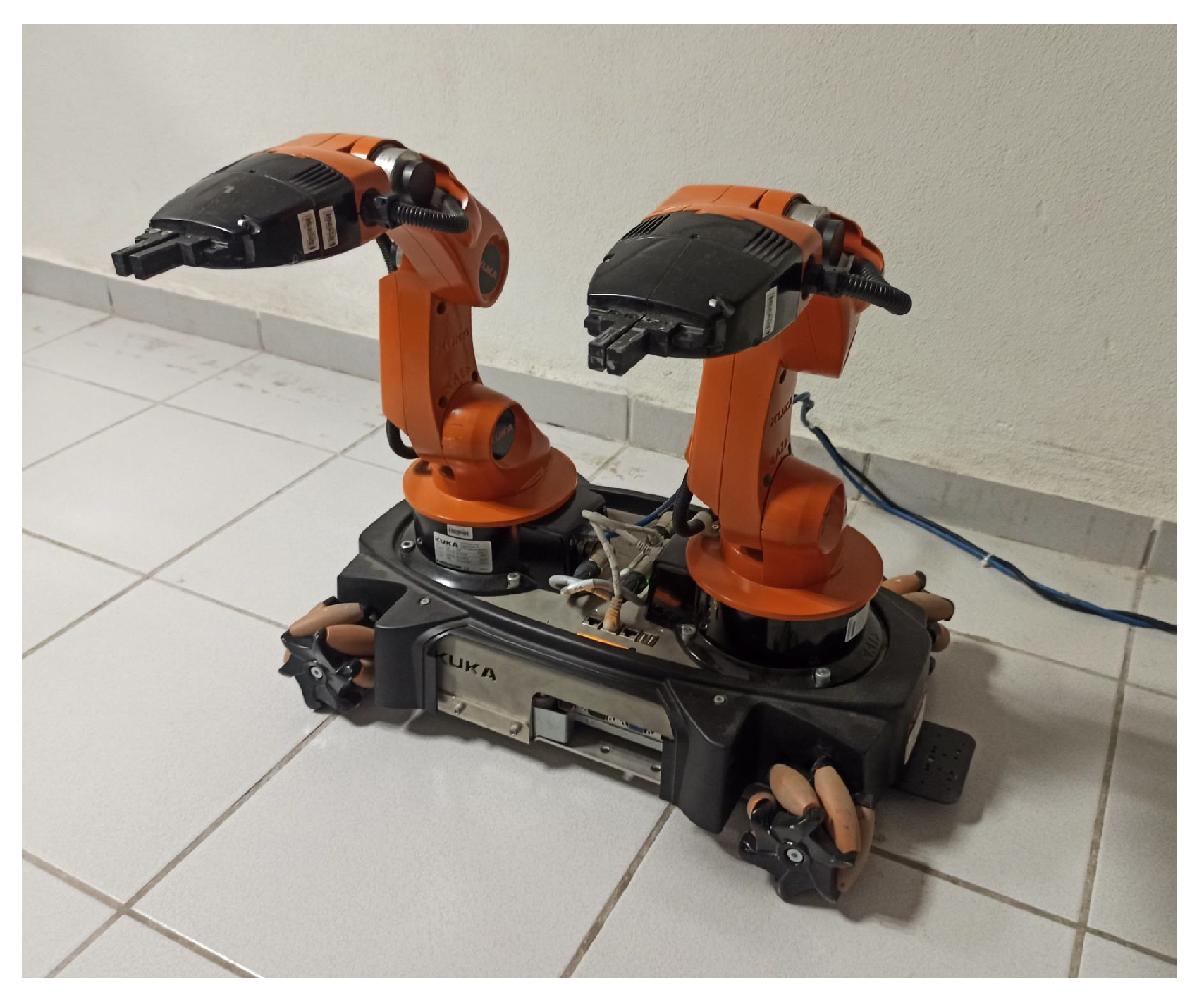
A mobile dual-arm system is composed of two manipulators attached to a mobile platform; see Figure 1. The two arms have similar kinematic structures, although they may be different. On the other hand, the mobile platform can represent a differential-drive robot, a car-like robot, or an omnidirectional robot. The advantage of using an omnidirectional robot over the other platforms is the movement capabilities that allow simultaneous displacements in any direction to reach any position and orientation in its operational space. In contrast, the differential-drive and car-like robots have limited movements due to their nonholonomic constraints [32].

In this work, we provide a kinematic model based on the KUKA^® Youbot^® robot [33]. This system is conformed by two identical manipulators of five DOFs composed of revolute joints and an omnidirectional mobile platform with three DOFs. Each manipulator is composed of revolute joints, and there is a gripper in the end-effector. The technical specification was carefully revised, and the kinematic analysis is given below.

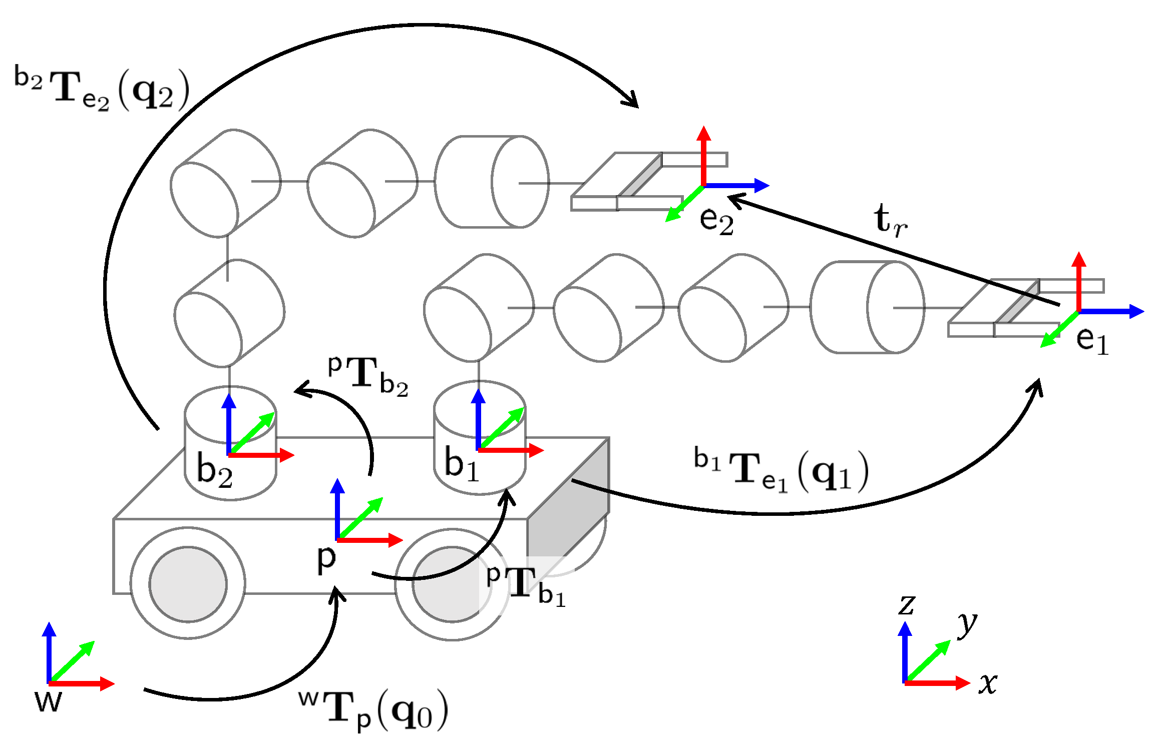
The kinematic chain of the considered mobile dual-arm system is described in Figure 2. Coordinate homogeneity is considered to establish the kinematic model. Then, the following frames are defined: $\left\{\mathsf{w}\right\}$ represents the world frame; $\left\{\mathsf{p}\right\}$ is a frame attached to the mobile platform; $\left\{{\mathsf{b}}_i\right\}$ is a frame attached to the beginning of the kinematic chain of the manipulator i; $\left\{{\mathsf{e}}_i\right\}$ is a frame attached to the end-effector, with $i=1,2$. Moreover, the pose of the mobile platform is represented by ${\mathbf{q}}_0$, and the homogeneous matrix ${}^{\mathsf{w}}{\mathbf{T}}_{\mathsf{p}}$ transforms the platform pose relative to the world frame $\left\{\mathsf{w}\right\}$. The matrix ${}^{\mathsf{p}}{\mathbf{T}}_{{\mathsf{b}}_i}$ is a constant transformation to adjust the distance among the $\left\{\mathsf{p}\right\}$ and $\left\{{\mathsf{b}}_i\right\}$ frames. Finally, ${\mathbf{q}}_i$ contains the joint configuration of the manipulator i, and the matrix ${}^{{\mathsf{b}}_i}{\mathbf{T}}_{{\mathsf{e}}_i}$ represents the forward kinematics of manipulator i. The vector ${\mathbf{t}}_r$ is defined for coordinated manipulation purposes, but we will talk about this in Section 3.

The pose of the mobile platform is described as

$${\mathbf{q}}_0={\left[\begin{array}{ccc}{x}_p& y_p& {\theta }_p\end{array}\right]}^T$$

(1)

where $x_p$ and $y_p$ are the platform position and ${\theta }_p$ its orientation. The matrix ${}^{\mathsf{w}}{\mathbf{T}}_{\mathsf{p}}$ can be defined as

$${}^{\mathsf{w}}{\mathbf{T}}_{\mathsf{p}}\left({\mathbf{q}}_0\right)=\left[\begin{array}{cccc}cos\left({\theta }_p\right)& -sin\left({\theta }_p\right)& 0& x_p\\ sin\left({\theta }_p\right)& cos\left({\theta }_p\right)& 0& y_p\\ 0& 0& 1& 0\\ 0& 0& 0& 1\end{array}\right]$$

(2)

The constant matrix ${}^{\mathsf{p}}{\mathbf{T}}_{{\mathsf{b}}_i}$ includes a rotation matrix ${}^{\mathsf{p}}{\mathbf{R}}_{{\mathsf{b}}_i}$ and a translation vector ${}^{\mathsf{p}}{\mathbf{t}}_{{\mathsf{b}}_i}$ to adjust the orientation and the position of frame $\left\{{\mathsf{b}}_i\right\}$ relative to frame $\left\{\mathsf{p}\right\}$. This transformation is shown below:

$${}^{\mathsf{p}}{\mathbf{T}}_{{\mathsf{b}}_i}=\left[\begin{array}{cc}{}^{\mathsf{p}}{\mathbf{R}}_{{\mathsf{b}}_i}& {}^{\mathsf{p}}{\mathbf{t}}_{{\mathsf{b}}_i}\\ \mathbf{0}& 1\end{array}\right]$$

(3)

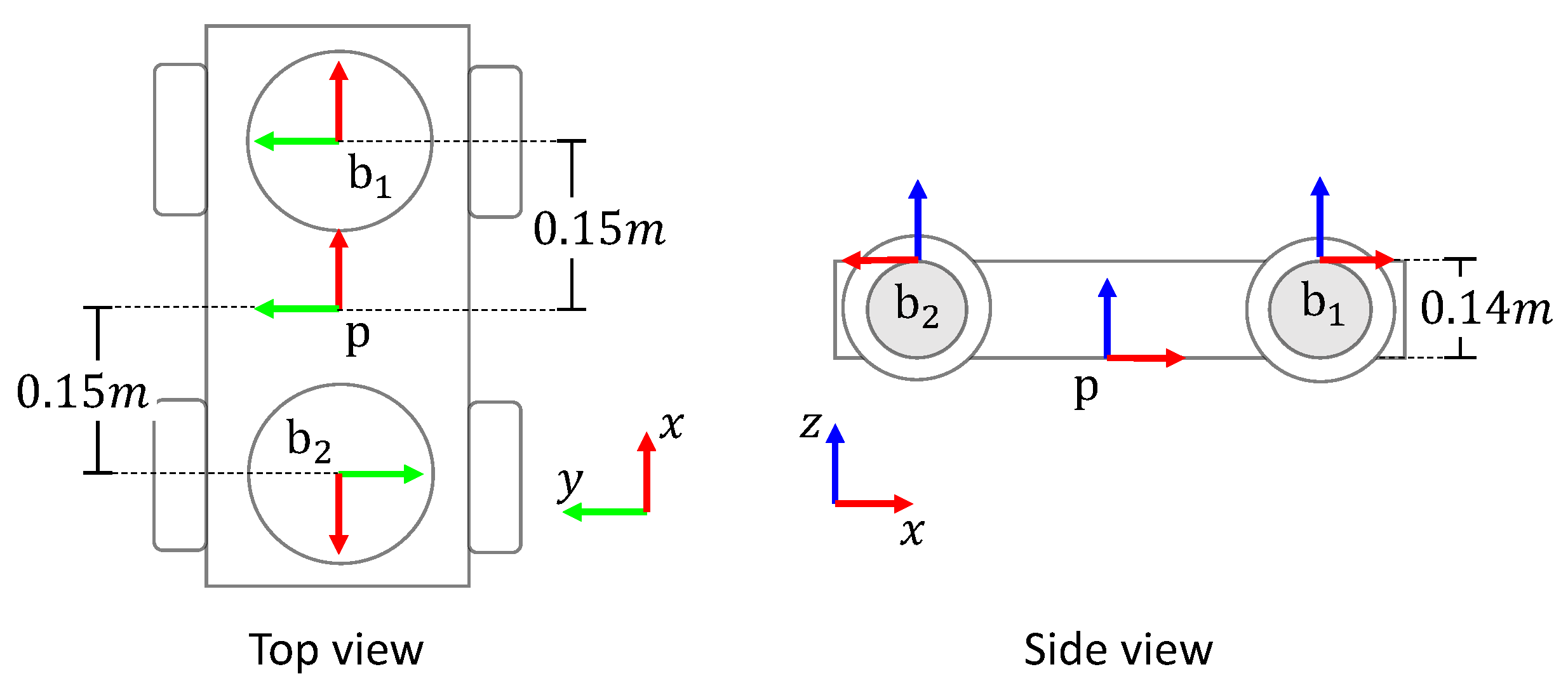
Figure 3 shows the coordinate frames assignment for the KUKA^® Youbot^® platform to obtain the matrices in (3). The frames $\left\{{\mathsf{b}}_i\right\}$ and $\left\{\mathsf{p}\right\}$ are also included. Based on the provided specifications, the following matrices are established:

$${}^{\mathsf{p}}{\mathbf{T}}_{{\mathsf{b}}_1}=\left[\begin{array}{cccc}1& 0& 0& 0.15\\ 0& 1& 0& 0\\ 0& 0& 1& 0.14\\ 0& 0& 0& 1\end{array}\right],{}^{\mathsf{p}}{\mathbf{T}}_{{\mathsf{b}}_2}=\left[\begin{array}{cccc}-1& 0& 0& -0.15\\ 0& -1& 0& 0\\ 0& 0& 1& 0.14\\ 0& 0& 0& 1\end{array}\right]$$

The joint configuration of manipulator i is described as

$${\mathbf{q}}_i={\left[\begin{array}{ccccc}{\theta }_1^i& {\theta }_2^i& {\theta }_3^i& {\theta }_4^i& {\theta }_5^i\end{array}\right]}^T$$

(4)

where ${\theta }_j^i$ represents the current joint value of the articulation j, where $j=1,2,3,4,5$. The forward kinematics ${}^{{\mathsf{b}}_i}{\mathbf{T}}_{{\mathsf{e}}_i}$ can be obtained based on the Denavit–Hartenberg (DH) model [5,34].

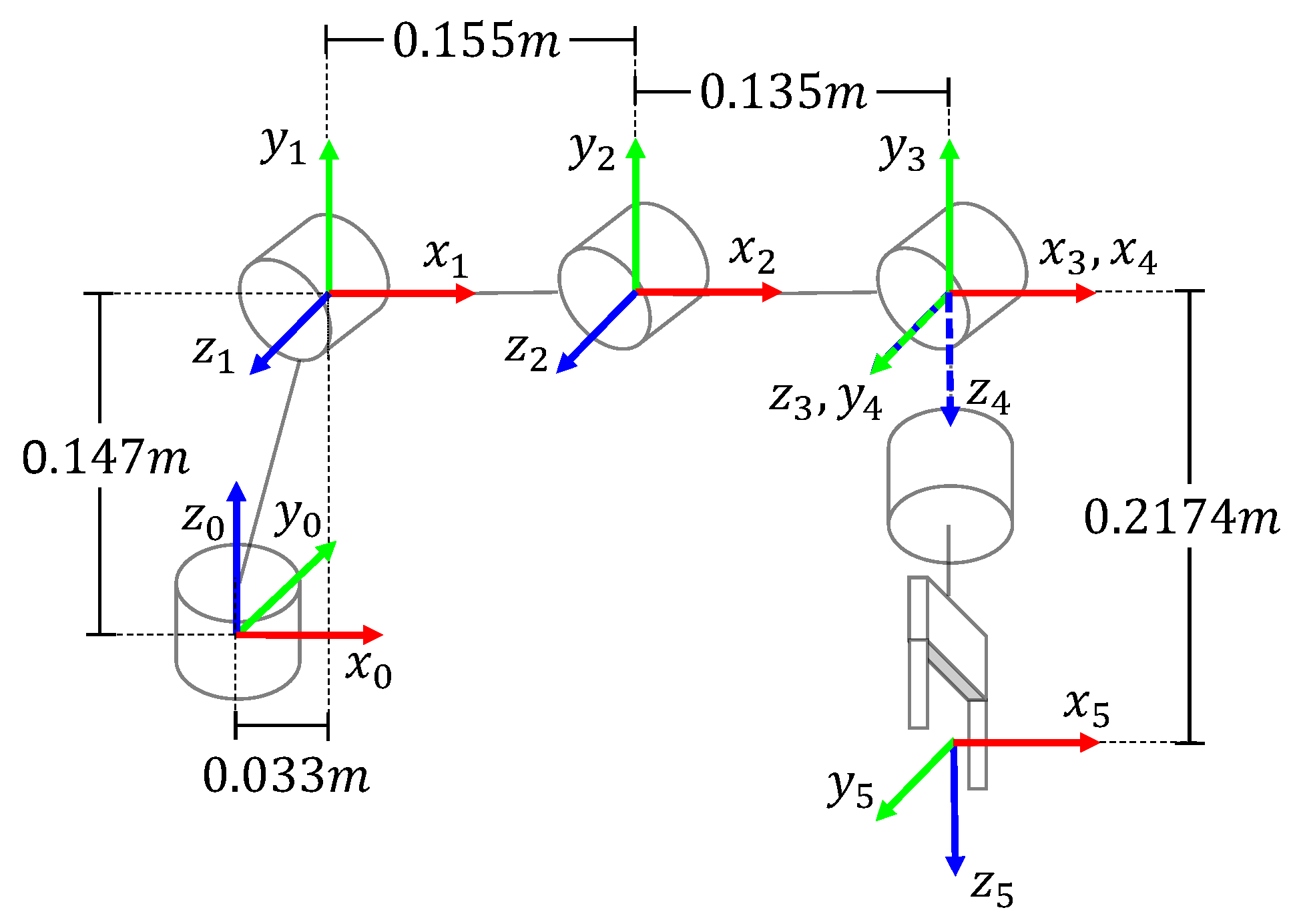
Figure 4 illustrates the coordinate frames’ assignment for the KUKA^® Youbot^® arm to obtain the DH table provided in

Table 2. DH table for the KUKA^® Youbot^® manipulator.

Link	a (m)	$\mathit{\alpha }$(rad)	d (m)	$\mathit{\theta }$ (rad)
1	0.033	$\pi /2$	0.147	${\theta }_1$
2	0.155	0	0	${\theta }_2$
3	0.135	0	0	${\theta }_3$
4	0	$\pi /2$	0	${\theta }_4$
5	0	0	0.2175	${\theta }_5$

. Each link j is represented by a homogeneous matrix ${}^{j-1}{\mathbf{T}}_j$, which transforms the frame attached to the link $j-1$ into the frame link j. The matrix ${}^{j-1}{\mathbf{T}}_j$ is expressed as

$${}^{j-1}{\mathbf{T}}_j=\left[\begin{array}{cccc}c{\theta }_j& -s{\theta }_{j}c{\alpha }_j& s{\theta }_{j}s{\alpha }_j& a_{j}c{\theta }_j\\ s{\theta }_j& c{\theta }_{j}c{\alpha }_j& -c{\theta }_{j}s{\alpha }_j& a_{j}s{\theta }_j\\ 0& s{\alpha }_j& c{\alpha }_j& d_j\\ 0& 0& 0& 1\end{array}\right]$$

(5)

where ${\theta }_j$ is a joint angle, $a_j$ is a link length, $d_j$ is a link offset, and ${\alpha }_j$ is a link twist. For brevity, the $sin$ and $cos$ operations are represented with the letters s and c, respectively.

Considering the parameters in Table 2 and using (5), the following matrices can be obtained:

$$\begin{array}{cc}\hfill {}^0{\mathbf{T}}_1\left({\theta }_1\right)& =\left[\begin{array}{cccc}cos\left({\theta }_1\right)& 0& sin\left({\theta }_1\right)& 0.033cos\left({\theta }_1\right)\\ sin\left({\theta }_1\right)& 0& -cos\left({\theta }_1\right)& 0.033sin\left({\theta }_1\right)\\ 0& 1& 0& 0.147\\ 0& 0& 0& 1\end{array}\right]\hfill \\ \hfill {}^1{\mathbf{T}}_2\left({\theta }_2\right)& =\left[\begin{array}{cccc}cos\left({\theta }_2\right)& -sin\left({\theta }_2\right)& 0& 0.155cos\left({\theta }_2\right)\\ sin\left({\theta }_2\right)& cos\left({\theta }_2\right)& 0& 0.155sin\left({\theta }_2\right)\\ 0& 0& 1& 0\\ 0& 0& 0& 1\end{array}\right]\hfill \\ \hfill {}^2{\mathbf{T}}_3\left({\theta }_3\right)& =\left[\begin{array}{cccc}cos\left({\theta }_3\right)& -sin\left({\theta }_3\right)& 0& 0.135cos\left({\theta }_3\right)\\ sin\left({\theta }_3\right)& cos\left({\theta }_3\right)& 0& 0.135sin\left({\theta }_3\right)\\ 0& 0& 1& 0\\ 0& 0& 0& 1\end{array}\right]\hfill \\ \hfill {}^3{\mathbf{T}}_4\left({\theta }_4\right)& =\left[\begin{array}{cccc}cos\left({\theta }_4\right)& 0& sin\left({\theta }_4\right)& 0\\ sin\left({\theta }_4\right)& 0& -cos\left({\theta }_4\right)& 0\\ 0& 1& 0& 0\\ 0& 0& 0& 1\end{array}\right]\hfill \\ \hfill {}^4{\mathbf{T}}_5\left({\theta }_5\right)& =\left[\begin{array}{cccc}cos\left({\theta }_5\right)& -sin\left({\theta }_5\right)& 0& 0\\ sin\left({\theta }_5\right)& cos\left({\theta }_5\right)& 0& 0\\ 0& 0& 1& 0.2175\\ 0& 0& 0& 1\end{array}\right]\hfill \end{array}$$

Then, the forward kinematics ${}^{{\mathsf{b}}_i}{\mathbf{T}}_{{\mathsf{e}}_i}\left({\mathbf{q}}_i\right)$ for each arm is calculated as

$${}^{{\mathsf{b}}_i}{\mathbf{T}}_{{\mathsf{e}}_i}\left({\mathbf{q}}_i\right)={}^0{\mathbf{T}}_5\left({\mathbf{q}}_i\right)={}^0{\mathbf{T}}_1{\left({\theta }_1^i\right)}^1{\mathbf{T}}_2{\left({\theta }_2^i\right)}^2{\mathbf{T}}_3{\left({\theta }_3^i\right)}^3{\mathbf{T}}_4{\left({\theta }_4^i\right)}^4{\mathbf{T}}_5\left({\theta }_5^i\right)$$

(6)

Given an actual pose of the platform ${\mathbf{q}}_0$ and a joint configuration of each manipulator ${\mathbf{q}}_i$, the forward kinematics of the mobile dual-arm system can be obtained as follows:

$${}^{\mathsf{w}}{\mathbf{T}}_{{\mathsf{e}}_i}\left({\mathbf{q}}_0,{\mathbf{q}}_i\right)={}^{\mathsf{w}}{\mathbf{T}}_{\mathsf{p}}\left({\mathbf{q}}_0\right){}^{\mathsf{p}}{\mathbf{T}}_{{\mathsf{b}}_i}{}^{{\mathsf{b}}_i}{\mathbf{T}}_{{\mathsf{e}}_i}\left({\mathbf{q}}_i\right)=\left[\begin{array}{cc}{}^{\mathsf{w}}{\mathbf{R}}_{{\mathsf{e}}_i}& {}^{\mathsf{w}}{\mathbf{t}}_{{\mathsf{e}}_i}\\ \mathbf{0}& 1\end{array}\right]$$

(7)

where ${}^{\mathsf{w}}{\mathbf{T}}_{{\mathsf{e}}_i}\left({\mathbf{q}}_0,{\mathbf{q}}_i\right)$ contains the position ${}^{\mathsf{w}}{\mathbf{t}}_{{\mathsf{e}}_i}$ and orientation ${}^{\mathsf{w}}{\mathbf{R}}_{{\mathsf{e}}_i}$ of the end-effector $\left\{{\mathsf{e}}_i\right\}$ with respect to the world frame $\left\{\mathsf{w}\right\}$.

The inverse kinematics of mobile dual-arm robots consists of computing the platform’s actual pose ${\mathbf{q}}_0$ and the joint configurations ${\mathbf{q}}_i$ given a desired end-effector pose ${}^{\mathsf{w}}{\mathbf{T}}_{{\mathsf{e}}_i}$ for each manipulator. This work proposes an algorithm to solve the inverse kinematics of mobile dual-arm robots for cooperative manipulation tasks.

3. Description of the Proposed Approach

In a mobile dual-arm cooperative system, the manipulators can interact with each other to solve coordinated manipulation or work independently to solve non-coordinated tasks. Moreover, both manipulators perform the manipulation tasks on board the same mobile platform. Indeed, this complicates the kinematics analysis for both coordinated and non-coordinated manipulation. The inverse kinematics for mobile dual-arm systems cannot be solved independently due to both manipulators sharing the same platform pose. This paper addresses the case of coordinated manipulation. However, this approach can also be applied to solve non-coordinated tasks.

The proposal is based on the forward kinematic equations considering the two manipulators and the mobile platform. Considering all as a whole system, the inverse kinematics gives the system configuration no matter if it is a coordinated or a non-coordinated task. On the other hand, considering the manipulators independently, they cannot achieve their objective due to the interaction with the robotic platform.

Let us consider the mobile dual-arm robot presented in Figure 2. For coordinated manipulation, we considered that manipulator 1 has the role of master. Then, a vector ${\mathbf{t}}_r$ is defined to compute the relative position of the end-effector $\left\{{\mathsf{e}}_2\right\}$ expressed with respect to the frame $\left\{{\mathsf{e}}_1\right\}$. Then, we define the desired position ${\mathbf{t}}_{{\mathsf{e}}_1}^{*}$ for the end-effector of arm 1. The desired position ${\mathbf{t}}_{{\mathsf{e}}_2}^{*}$ for the end-effector of arm 2 is given by

$${\mathbf{t}}_{{\mathsf{e}}_2}^{*}={\mathbf{t}}_{{\mathsf{e}}_1}^{*}+{\mathbf{t}}_r$$

(8)

For non-coordinated manipulation, the desired position ${\mathbf{t}}_{{\mathsf{e}}_2}^{*}$ is provided independently of the desired position ${\mathbf{t}}_{{\mathsf{e}}_1}^{*}$.

3.1. Objective Function Formulation

The aim of the proposed inverse kinematics algorithm is to minimize the error between the desired end-effector position of each arm and the actual end-effectors’ positions. Furthermore, it is considered to minimize the error between current and previous joints, including the mobile platform poses. This is useful to reduce the system motion, especially during coordinated trajectory tracking tasks.

The error between the desired position ${\mathbf{t}}_{{\mathsf{e}}_i}^{*}$ and the actual position ${}^{\mathsf{w}}{\mathbf{t}}_{{\mathsf{e}}_i}$ of manipulator i can be computed as

$$e_{t_i}=∥{\mathbf{t}}_{{\mathsf{e}}_i}^{*}-{}^{\mathsf{w}}{\mathbf{t}}_{{\mathsf{e}}_i}∥$$

(9)

where $∥·∥$ denotes the Euclidean norm. The position ${}^{\mathsf{w}}{\mathbf{t}}_{{\mathsf{e}}_i}$ is obtained based on the forward kinematics (7) for the actual system configuration $\left({\mathbf{q}}_0,{\mathbf{q}}_i\right)$.

To minimize the coordinated manipulation motion, we define errors between the actual configurations $\left({\mathbf{q}}_0,{\mathbf{q}}_i\right)$ and the previous configurations $\left({\mathbf{q}}_0^{prev},{\mathbf{q}}_i^{prev}\right)$. These errors are defined as

$$\begin{array}{cc}\hfill e_{q_0}& =∥{\mathbf{q}}_0-{\mathbf{q}}_0^{prev}∥\hfill \\ \hfill e_{q_i}& =∥{\mathbf{q}}_i-{\mathbf{q}}_i^{prev}∥\hfill \end{array}$$

(10)

The formulation of an objective function f, which includes the position and motion errors, is defined as

$$f=\alpha \left(e_{t_1}+e_{t_2}\right)+\beta e_{q_0}+\gamma \left(e_{q_1}+e_{q_2}\right)$$

(11)

where $\alpha$, $\beta$, and $\gamma$ are positive factors to scale the contribution of each term. The larger the value of $\alpha$ is, the higher the priority to minimize position errors. The larger the values of $\beta$ are, the less movement for the mobile platform. Similarly, the larger the values of $\gamma$ are, the less movement for the joints of each arm. These factors can be selected experimentally, but we recommend $\alpha >\gamma >\beta$. That is, we provide higher priority to position errors, less motion for the manipulators, and much for the platform.

3.2. Inverse Kinematics Based on Metaheuristics Optimization Algorithms

We propose to solve the objective function (11) using metaheuristics algorithms. Most metaheuristics strategies are population-based optimization algorithms, where every member represents a potential solution. In this case, a population member contains a candidate configuration of the mobile dual-arm system. Moreover, metaheuristics algorithms require random initializations inside of a search space.

The joint rotation limits bound the search space of metaheuristics algorithms. The KUKA^® Youbot^® technical specifications provide the following upper ${\mathbf{q}}_{i_u}$ and lower ${\mathbf{q}}_{i_u}$ joint limits.

$$\begin{array}{cc}\hfill {\mathbf{q}}_{1_l}& ={\mathbf{q}}_{2_l}={\left[\begin{array}{ccccc}-{169}^{\circ }& -{65}^{\circ }& -{150}^{\circ }& -{102.5}^{\circ }& -{167.5}^{\circ }\end{array}\right]}^T\hfill \\ \hfill {\mathbf{q}}_{1_u}& ={\mathbf{q}}_{2_u}={\left[\begin{array}{ccccc}{169}^{\circ }& {90}^{\circ }& {146}^{\circ }& {102.5}^{\circ }& {167.5}^{\circ }\end{array}\right]}^T\hfill \end{array}$$

The translations of the mobile platform and its rotation have no limits. However, we propose the following workspace to keep the platform movements bounded:

$$\begin{array}{cc}\hfill {\mathbf{q}}_{0_l}& ={\left[\begin{array}{ccc}-1.5m& -1.5m& -{180}^{\circ }\end{array}\right]}^T\hfill \\ \hfill {\mathbf{q}}_{0_u}& ={\left[\begin{array}{ccc}1.5m& 1.5m& {180}^{\circ }\end{array}\right]}^T\hfill \end{array}$$

where ${\mathbf{q}}_{0_l}$ and ${\mathbf{q}}_{0_u}$ are the lower and upper boundaries, respectively. All lower and upper boundaries are shown in degree values for clarity, although in the optimization process, the algorithms use radians. Then, we define the lower and upper boundaries of the whole mobile dual-arm system as ${\mathbf{q}}_l={\left[\begin{array}{ccc}{\mathbf{q}}_{0_l}^T& {\mathbf{q}}_{1_l}^T& {\mathbf{q}}_{2_l}^T\end{array}\right]}^T$ and ${\mathbf{q}}_u={\left[\begin{array}{ccc}{\mathbf{q}}_{0_u}^T& {\mathbf{q}}_{1_u}^T& {\mathbf{q}}_{2_u}^T\end{array}\right]}^T$, respectively. These boundaries are needed to randomly initialize candidate solutions. Moreover, ${\mathbf{q}}_l,{\mathbf{q}}_u\in {\mathbb{R}}^D$, where $D=13$ is the dimension of the optimization problem.

To generate random solutions, we propose to use the following equation:

$${\mathbf{q}}_r={\mathbf{q}}_l+\left({\mathbf{q}}_u-{\mathbf{q}}_l\right)\odot \mathbf{r}$$

(12)

where ⊙ indicates the elementwise product and $\mathbf{r}\in {\mathbb{R}}^D$ is a uniformly distributed random vector, where each element is in the range $[0,1]$. The random vector ${\mathbf{q}}_r$ represents an initial solution for a candidate configuration.

The lower and upper boundaries also represent constraints that must be considered for real-world implementations. We considered solving the inverse kinematics of mobile dual-arm robots as a global constrained optimization problem, which is expressed as

$$\begin{array}{c}\underset{\mathbf{q}}{arg\; min}f\left(\mathbf{q}\right),\mathrm{subject}\mathrm{to}{\mathbf{q}}_l<\mathbf{q}<{\mathbf{q}}_u\end{array}$$

(13)

where $\mathbf{q}$ defines the optimal configuration of the mobile dual-arm system with $\mathbf{q}={\left[\begin{array}{ccc}{\mathbf{q}}_0^T& {\mathbf{q}}_1^T& {\mathbf{q}}_2^T\end{array}\right]}^T$. The set of solutions that satisfy $\mathbf{F}=\left\{\mathbf{q}:{\mathbf{q}}_l<\mathbf{q}<{\mathbf{q}}_u\right\}$ is called the feasible solutions. In contrast, unfeasible solutions are given by $\overline{\mathbf{F}}=\left\{\mathbf{q}:\mathbf{q}\notin \mathbf{F}\right\}$. To deal with the constraints, we recalculated the vector $\mathbf{q}$ for those infeasible solutions using (12).

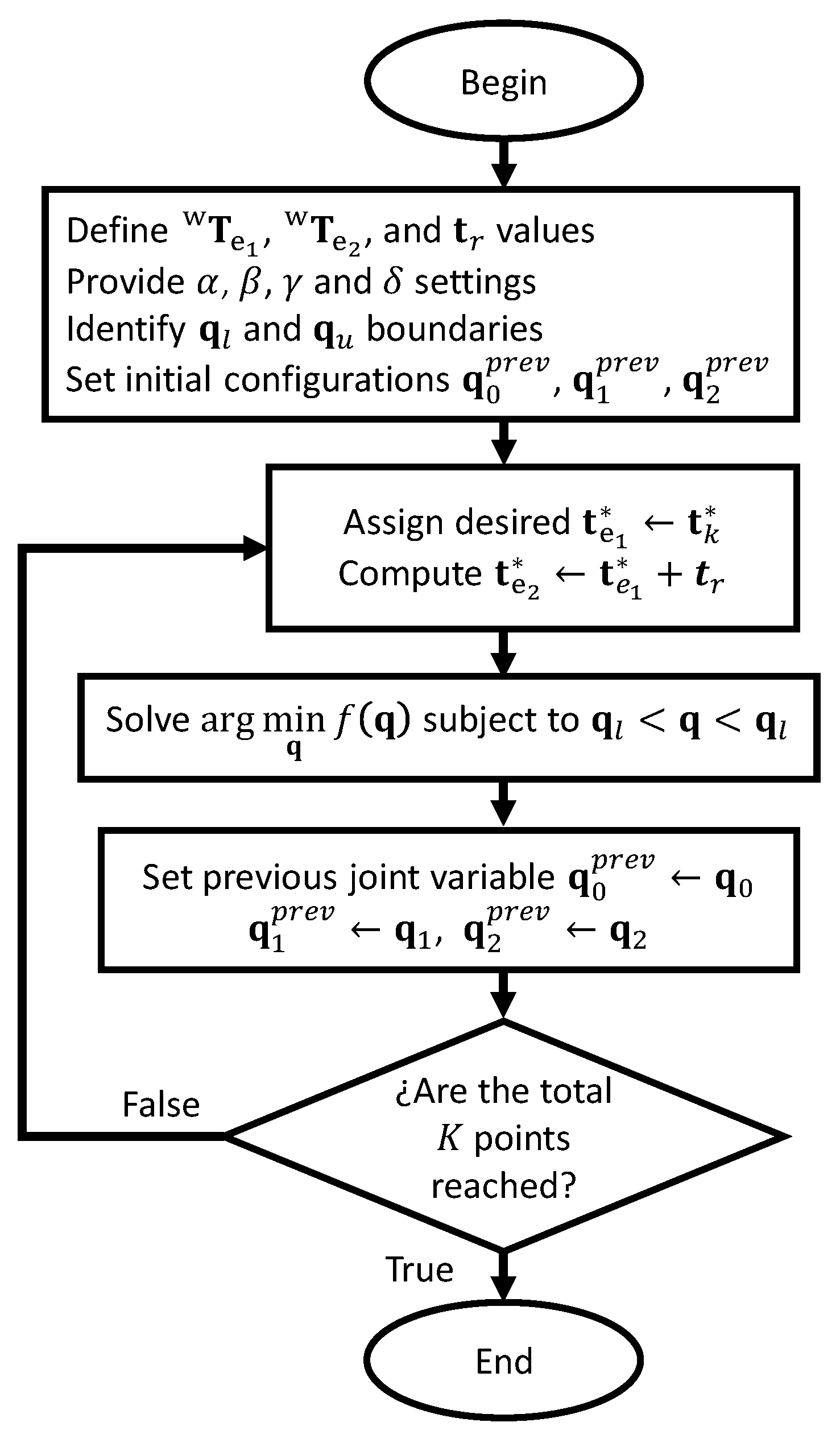
3.3. Coordinated Trajectory Tracking Algorithm

A path is divided into K points to solve coordinated trajectory tracking tasks. Every point $k=1,2,3,\cdots ,K$ becomes a desired position ${\mathbf{t}}_k^{*}$ for end-effector 1. The relative desired position for end-effector 2 is computed using (8). Then, the inverse kinematics is solved based on the optimization problem expressed in (13) to obtain an optimal configuration ${\mathbf{q}}_k$. The solution ${\mathbf{q}}_k$ becomes the previous configuration for the next desired point ${\mathbf{t}}_{k+1}^{*}$. The goal is to find the set of solutions $\mathbf{Q}=\left\{{\mathbf{q}}_1,{\mathbf{q}}_2,{\mathbf{q}}_3,\cdots ,{\mathbf{q}}_K\right\}$ that define the trajectory tracking. A summary of the proposed coordinated trajectory tracking algorithm is given in Figure 5.

4. Experimental Results

The experiments aimed to test the performance of the proposed inverse kinematics of mobile dual-arm robots for cooperative manipulation. The considered tasks are coordinated inverse kinematics and coordinated trajectory tracking. The applicability of the proposed approach is demonstrated using the mobile dual-arm system based on the KUKA^® Youbot^® robot. Moreover, the tests were conducted in simulations and real-world experiments.

For the coordinated inverse kinematics tests, we propose to use the following desired positions.

$$\begin{array}{cc}\hfill & \mathrm{Target}\mathrm{point}1:\hfill \\ \hfill {\mathbf{t}}_r& ={\left[\begin{array}{ccc}0.2& -0.3& -0.2\end{array}\right]}^T\hfill \\ \hfill {\mathbf{t}}_{{\mathsf{e}}_1}^{*}& ={\left[\begin{array}{ccc}0.5& -0.2& 0.45\end{array}\right]}^T\hfill \\ \hfill \\ \hfill & \mathrm{Target}\mathrm{point}3:\hfill \\ \hfill {\mathbf{t}}_r& ={\left[\begin{array}{ccc}-0.2& -0.5& -0.1\end{array}\right]}^T\hfill \\ \hfill {\mathbf{t}}_{{\mathsf{e}}_1}^{*}& ={\left[\begin{array}{ccc}0.5& 0.2& 0.4\end{array}\right]}^T\hfill \end{array}\begin{array}{cc}\hfill & \mathrm{Target}\mathrm{point}2:\hfill \\ \hfill {\mathbf{t}}_r& ={\left[\begin{array}{ccc}0.0& -0.5& 0.0\end{array}\right]}^T\hfill \\ \hfill {\mathbf{t}}_{{\mathsf{e}}_1}^{*}& ={\left[\begin{array}{ccc}0.3& 0.2& 0.5\end{array}\right]}^T\hfill \\ \hfill \\ \hfill & \mathrm{Target}\mathrm{point}4:\hfill \\ \hfill {\mathbf{t}}_r& ={\left[\begin{array}{ccc}0.0& -0.3& 0.2\end{array}\right]}^T\hfill \\ \hfill {\mathbf{t}}_{{\mathsf{e}}_1}^{*}& ={\left[\begin{array}{ccc}-0.25& 0.3& 0.3\end{array}\right]}^T\hfill \end{array}$$

Four trajectories with different difficulty degrees are defined for coordinate trajectory tracking. Each trajectory was divided into $K=200$ points. The vector ${\mathbf{t}}_k^{*}={\left[\begin{array}{ccc}{x}_k& y_k& z_k\end{array}\right]}^T$ defines the k-th trajectory point. The trajectories are

$$\begin{array}{cc}\hfill & \mathrm{Trajectory}1:\mathrm{Sinusoidal}\hfill \\ \hfill x_k& =0.5\hfill \\ \hfill z_k& =0.4+0.05sin\left(30y_k\right)\hfill \\ \hfill y_k& \in \left[-0.25,0.75\right]\hfill \\ \hfill \\ \hfill & \mathrm{Trajectory}3:\mathrm{Trapezoidal}\hfill \\ \hfill x_k& =0.5\hfill \\ \hfill r_k& =0.45+0.1sin\left(30y_k\right)\hfill \\ \hfill y_k& \in \left[-0.25,0.75\right]\hfill \\ \hfill z_k& =\left\{\begin{array}{ccc}0.5& & \mathrm{if}{r}_k>0.5\\ 0.4& & \mathrm{if}{r}_k<0.4\\ r_k& & \mathrm{otherwise}\end{array}\right.\hfill \end{array}\begin{array}{cc}\hfill & \mathrm{Trajectory}2:\mathrm{Circular}\hfill \\ \hfill x_k& =0.5\hfill \\ \hfill y_k& =0.25+0.05cos\left({\theta }_k\right)\hfill \\ \hfill z_k& =0.45+0.05sin\left({\theta }_k\right)\hfill \\ \hfill {\theta }_k& \in \left[0,2\pi \right]\hfill \\ \hfill \\ \hfill & \mathrm{Trajectory}4:\mathrm{Rose}\mathrm{curve}\hfill \\ \hfill x_k& =0.5\hfill \\ \hfill y_k& =0.25+r_{k}cos\left({\theta }_k\right)\hfill \\ \hfill z_k& =0.35+r_{k}sin\left({\theta }_k\right)\hfill \\ \hfill r_k& =0.035+0.015cos\left(3{\theta }_k\right)\hfill \\ \hfill {\theta }_k& \in \left[0,2\pi \right]\hfill \end{array}$$

For all experiments, the parameter settings related to the objective function were selected as $\alpha =1.2$, $\beta =0.1$, and $\gamma =0.4$. These values were selected experimentally, but we ensured that $\alpha >\gamma >\beta$. Moreover, the following initial configurations were fixed as

$$\begin{array}{cc}\hfill {\mathbf{q}}_0^{prev}& ={\left[\begin{array}{ccc}0& 0& \pi /2\end{array}\right]}^T\hfill \\ \hfill {\mathbf{q}}_1^{prev}& ={\left[\begin{array}{ccccc}-\pi /2& \pi /2& -\pi /4& \pi /4& 0\end{array}\right]}^T\hfill \\ \hfill {\mathbf{q}}_2^{prev}& ={\left[\begin{array}{ccccc}\pi /2& \pi /2& -\pi /4& \pi /4& 0\end{array}\right]}^T\hfill \end{array}$$

The performance of the proposed approach was analyzed and compared using the following metaheuristics algorithms: DE, CPABC, SDE, CS, QPSO, IMPSO, and CMA-ES. The comparisons were performed to find the algorithm that best minimizes the position and motion errors.

The parameter settings for the considered metaheuristics were conducted as follows: First, the common parameters were the population size of 30 members and a total of 1000 iterations. The particular parameter settings are given in

Table 3. Parameter settings in state-of-the-art literature review.

Reference	Algorithm	Parameter Settings
[28]	DE	DE/rand/1/bin, $F=0.6$, $C_R=0.9$
[21]	CPABC	Limits $L=40$, $M_R=0.8$, $S_F=0.6$
[30]	SDE	$F=0.5$, $C_R=0.8$
[26]	CS	Discover rate $P=0.25$
[20]	QPSO	${\beta }_0=0.5$, ${\beta }_1=1.0$
[17]	IMPSO	$w_i=\left\{0.2,0.4,0.6,0.8,1.0,1.2,1.4,1.6,1.8,2.0\right\}$, $C_1=1.4962$, $C_2=1.4962$
[27]	CMAES	Standard $(\mu ,\lambda )$-CMA-ES, $\lambda =30$

.

The metaheuristics algorithms presented in Table 3 were considered for comparison purposes because they have been used previously in the literature to solve the inverse kinematics of fixed robotics manipulators, as reported in the following works [17,18,21,26,27,28,30].

In all experiments, the specifications of the test machine were an Intel Core i7-4770^® (Intel i7 is a registered trademark of Intel Corporation USA) CPU $3.4$ GHz and 16 GB of RAM. Moreover, the experiments were performed in the Matlab R2021a environment^® (Matlab is a registered trademark of the MathWorks, Inc., USA).

4.1. Simulation Experiments for Coordinated Inverse Kinematics

This section presents a comparative analysis of different metaheuristics optimization algorithms for solving coordinated inverse kinematics tasks. The aim of the simulations was to identify those algorithms that best minimized the position errors $e_{t_1}$ and $e_{t_2}$. The best algorithms are compared later in coordinated trajectory tracking tasks to analyze the motion error results.

For comparison purposes, every metaheuristic ran 100 times independently. To qualify the results, the statistical performance was measured with the mean, standard deviation (STD), and the best and worst results. The best algorithms report a small mean value with a low standard distribution, which is a small difference between the best and worst results. These measures are shown in tables, where the position error reported is $e_{t_1}+e_{t_2}$, which is given in meters (m).

In these tests, we considered that a coordinated inverse kinematics task is successfully solved if the reported position error result is less than $1\times {10}^{-4}$, which is an error below $0.1$ mm. Then, a mean value below $1\times {10}^{-4}$ indicates accurate results. Moreover, a low STD value indicates better precision. Additionally, the difference between the best and the worst measures shows the amount of dispersion related to the accuracy.

The coordinated inverse kinematics results are provided in

Table 4. Position error results for target point 1. The best results are highlighted in bold.

	DE	CPABC	SDE	CS	QPSO	IMPSO	CMA-ES
Mean	5.136 $\times {10}^{-6}$	0.022031	5.440 $\times {10}^{-7}$	0.00013183	0.0008852	0.0018518	$\mathbf{7.965}\times {10}^{-15}$
STD	2.360 $\times {10}^{-5}$	0.097928	1.193 $\times {10}^{-6}$	6.929 $\times {10}^{-5}$	0.0037455	0.0084942	$\mathbf{1.509}\times {10}^{-14}$
Best	7.488 $\times {10}^{-9}$	1.717 $\times {10}^{-15}$	3.683 $\times {10}^{-9}$	2.513 $\times {10}^{-5}$	$\mathbf{6.245}\times {10}^{-17}$	8.370 $\times {10}^{-17}$	6.973 $\times {10}^{-16}$
Worst	0.00016689	0.58487	6.887$\times {10}^{-6}$	0.0003229	0.022734	0.055906	$\mathbf{1.03}\times {10}^{-13}$

,

Table 5. Position error results for target point 2. The best results are highlighted in bold.

	DE	CPABC	SDE	CS	QPSO	IMPSO	CMA-ES
Mean	1.036 $\times {10}^{-5}$	0.00051808	2.768 $\times {10}^{-6}$	0.0003566	0.0002991	0.0062474	$\mathbf{3.803}\times {10}^{-13}$
STD	2.287 $\times {10}^{-5}$	0.0018515	5.428 $\times {10}^{-6}$	0.00021011	0.00099298	0.035237	$\mathbf{1.469}\times {10}^{-12}$
Best	1.257 $\times {10}^{-8}$	7.467 $\times {10}^{-15}$	1.049 $\times {10}^{-8}$	9.012 $\times {10}^{-5}$	1.875 $\times {10}^{-13}$	$\mathbf{1.746}\times {10}^{-16}$	4.616$\times {10}^{-16}$
Worst	0.00010999	0.011715	3.109 $\times {10}^{-5}$	0.0010176	0.0062429	0.24645	$\mathbf{8.107}\times {10}^{-12}$

,

Table 6. Position error results for target point 3. The best results are highlighted in bold.

	DE	CPABC	SDE	CS	QPSO	IMPSO	CMA-ES
Mean	8.119 $\times {10}^{-6}$	0.0036393	2.754 $\times {10}^{-6}$	0.00026886	0.0002542	0.0034882	$\mathbf{8.839}\times {10}^{-13}$
STD	1.843 $\times {10}^{-5}$	0.021661	5.134 $\times {10}^{-6}$	0.00016798	0.001258	0.020727	$\mathbf{2.685}\times {10}^{-12}$
Best	5.514 $\times {10}^{-8}$	7.992 $\times {10}^{-15}$	2.743 $\times {10}^{-8}$	3.107 $\times {10}^{-5}$	1.257 $\times {10}^{-13}$	$\mathbf{2.310}\times {10}^{-16}$	1.994 $\times {10}^{-15}$
Worst	0.00011067	0.15316	2.599 $\times {10}^{-5}$	0.00074317	0.0085917	0.14618	$\mathbf{1.523}\times {10}^{-11}$

and

Table 7. Position error results for target point 4. The best results are highlighted in bold.

	DE	CPABC	SDE	CS	QPSO	IMPSO	CMA-ES
Mean	4.213 $\times {10}^{-6}$	0.02832	3.229 $\times {10}^{-6}$	0.00043625	0.023282	0.040247	$\mathbf{8.710}\times {10}^{-14}$
STD	5.632 $\times {10}^{-6}$	0.087143	1.264 $\times {10}^{-5}$	0.00028418	0.015985	0.09733	$\mathbf{2.608}\times {10}^{-13}$
Best	8.997 $\times {10}^{-8}$	1.023 $\times {10}^{-15}$	1.919 $\times {10}^{-9}$	5.754 $\times {10}^{-5}$	5.658 $\times {10}^{-12}$	$\mathbf{7.850}\times {10}^{-17}$	8.01 $\times {10}^{-16}$
Worst	2.941 $\times {10}^{-5}$	0.39983	8.697 $\times {10}^{-5}$	0.0014147	0.064859	0.4156	$\mathbf{1.488}\times {10}^{-12}$

. CMA-ES showed the highest precision and accuracy in all cases. It showed the lowest mean and STD values. It also showed the smallest worst measures. Clearly, CMA-ES outperformed the other algorithms. The performances of DE and SDE were quite similar. Their results were precise and accurate. DE and SDE stood out with all measured values below $1\times {10}^{-4}$. The worst results of Table 4, Table 5 and Table 6 indicated that SDE performed slightly better than DE. QPSO presented the best measure in Table 4. Moreover, IMPSO showed the bests measures in Table 5, Table 6 and Table 7. The performances of QPSO and IMPSO were similar, but not the best. All mean and STD measures of IMPSO were higher than $1\times {10}^{-4}$, which means low precision and accuracy. Table 7 indicates that QPSO also had low precision and accuracy. CS showed balanced results. The results were accurate even if they did not demonstrate the best mean and STD values. In all tests, those results are provided below $1\times {10}^{-4}$. CPABC performed poorly in all tests. It did not provide precise nor accurate results. In almost all cases, the measured values presented were above $1\times {10}^{-4}$.

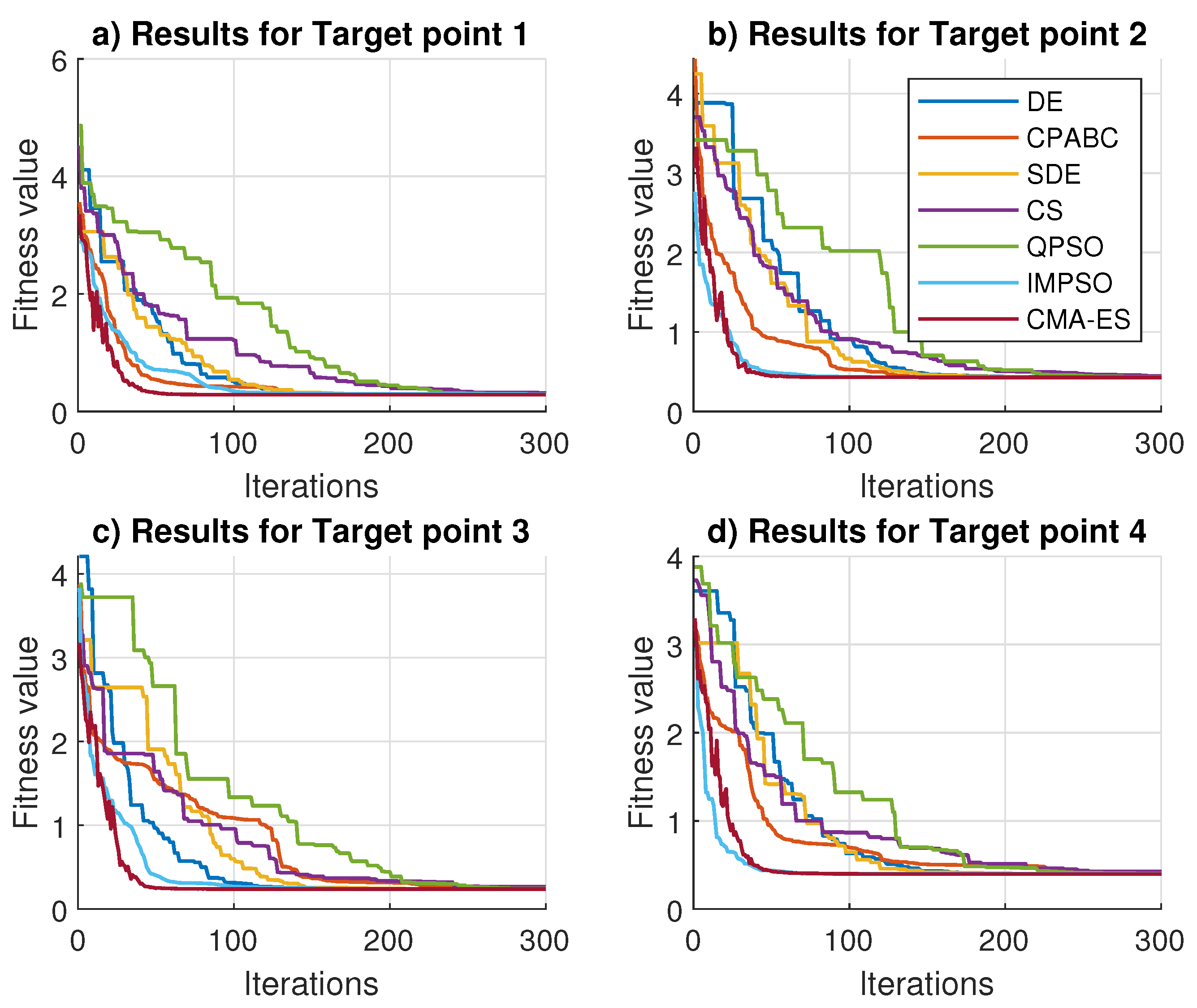
Figure 6 illustrates the convergence curves of all compared algorithms. These results were the fitness convergence rates for the best position error results. The graphs show the first 300 iterations because posterior results did not report significant differences. As can be seen, the fastest convergence rates were given by CMA-ES. IMPSO also had fast convergence, as shown in Figure 6b–d. Moreover, the converge curves of DE, CS, CPABC, and SDE were similar. Finally, the slowest convergence rate was provided by QPSO.

Based on the results of these tests, we noticed that CMA-ES outperformed the other algorithms. It showed the highest accuracy and precise results with faster convergence rates. Moreover, the performances of DE and SDE were also remarkable. The performance of CS stood out over IMPSO, QPSO, and CPABC. Finally, the IMPSO, QPSO, and CPABC algorithms were not considered for further comparison tests because of their poor performance.

4.2. Simulation Experiments for Coordinated Trajectory Tracking

This section presents the simulation results for coordinated trajectory tracking tasks. We compared the performance of the metaheuristics algorithms that best performed in the coordinated inverse kinematics tests. The compared algorithms were DE, SDE, CS, and CMA-ES. We were interested in finding the algorithm that best minimized the position errors $e_{t_1}$ and $e_{t_2}$, but also presented minimum motion errors $e_{q_0}$, $e_{q_1}$, and $e_{q_2}$. The best algorithm was used for the real-world implementations.

For the comparison analysis, the position errors are reported as $e_{t_1}+e_{t_2}$ and the motion errors as $e_{q_0}+e_{q_1}+e_{q_2}$. We used boxplots to graphically show the statistical variation of the inverse kinematics results related to each point in the trajectory. The best algorithms show a small data dispersion with a low median value. In addition, these results should present the fewest outliers.

In these simulations, the position and motion errors were compared using boxplots. To qualify the position error results, the statistical performance was measured with the mean, STD, and min and max value results. Moreover, the motion errors are illustrated with graphs to visually analyze the motion during the training tasks. Additionally, the desired trajectory and the actual trajectory provided by the optimization algorithms are also compared with graphs. Finally, each metaheuristics algorithm used a total of 300 iterations.

The position error results of the coordinated trajectory tasks are given in Figure 7. Clearly, CS showed the worst results. It had a larger data dispersion with the presence of outliers. In all cases, the reported median value was around $0.01$ m, which is not adequate for trajectory tracking. Moreover, it seems that DE, SDE, and CMAES performed similarly. They provided a small data dispersion with lower median values. However, these results are analyzed in tables for a fair comparison. Such results are given in

Table 8. Position error results for sinusoidal trajectory. The best results are highlighted in bold.

	DE	SDE	CS	CMA-ES
Mean	5.104 $\times {10}^{-5}$	5.5523 $\times {10}^{-5}$	0.0099478	$\mathbf{1.1142}\times {10}^{-8}$
STD	7.5244 $\times {10}^{-5}$	3.94 $\times {10}^{-5}$	0.0055781	$\mathbf{2.9257}\times {10}^{-8}$
Min	6.0195 $\times {10}^{-6}$	4.3216 $\times {10}^{-6}$	0.0028493	$\mathbf{2.6832}\times {10}^{-13}$
Max	0.00087922	0.00026586	0.036553	$\mathbf{3.7112}\times {10}^{-7}$

,

Table 9. Position error results for circular trajectory. The best results are highlighted in bold.

	DE	SDE	CS	CMA-ES
Mean	4.0829 $\times {10}^{-5}$	5.2769 $\times {10}^{-5}$	0.009863	$\mathbf{3.4473}\times {10}^{-9}$
STD	2.9189 $\times {10}^{-5}$	3.8536 $\times {10}^{-5}$	0.0046131	$\mathbf{6.085}\times {10}^{-9}$
Min	3.7308 $\times {10}^{-6}$	6.9321 $\times {10}^{-6}$	0.0025768	$\mathbf{3.7374}\times {10}^{-15}$
Max	0.00021541	0.0002404	0.027738	$\mathbf{4.8502}\times {10}^{-8}$

,

Table 10. Position error results for trapezoidal trajectory. The best results are highlighted in bold.

	DE	SDE	CS	CMA-ES
Mean	4.1641 $\times {10}^{-5}$	4.6393 $\times {10}^{-5}$	0.010247	$\mathbf{7.3893}\times {10}^{-9}$
STD	3.4045 $\times {10}^{-5}$	3.4973 $\times {10}^{-5}$	0.0047796	$\mathbf{2.0364}\times {10}^{-8}$
Min	4.1663 $\times {10}^{-6}$	5.7924 $\times {10}^{-6}$	0.0015987	$\mathbf{3.4801}\times {10}^{-16}$
Max	0.00024229	0.00019833	0.030391	$\mathbf{1.2199}\times {10}^{-7}$

and

Table 11. Position error results for rose curve trajectory. The best results are highlighted in bold.

	DE	SDE	CS	CMA-ES
Mean	3.5829 $\times {10}^{-5}$	4.2613 $\times {10}^{-5}$	0.0092417	$\mathbf{2.3824}\times {10}^{-9}$
STD	2.8703 $\times {10}^{-5}$	2.9939 $\times {10}^{-5}$	0.0048608	$\mathbf{3.9706}\times {10}^{-9}$
Min	5.3653 $\times {10}^{-6}$	4.1256 $\times {10}^{-6}$	0.0014107	$\mathbf{3.6486}\times {10}^{-12}$
Max	0.0001964	0.00018327	0.031768	$\mathbf{2.4175}\times {10}^{-8}$

.

Based on the results provided in Table 8, Table 9, Table 10 and Table 11, we noticed that the CMA-ES algorithm outperformed the others. It had the best mean, STD, and min and max results. These demonstrated that CMA-ES provided accurate and precise coordinate tracking results. DE and SDE also provided acceptable results with high accuracy and precision. They performed similarly in all cases, with measures below $1\times {10}^{-4}$. The performance of CS was poor. All reported measures were bigger than $1\times {10}^{-4}$, which demonstrated low accuracy and precision.

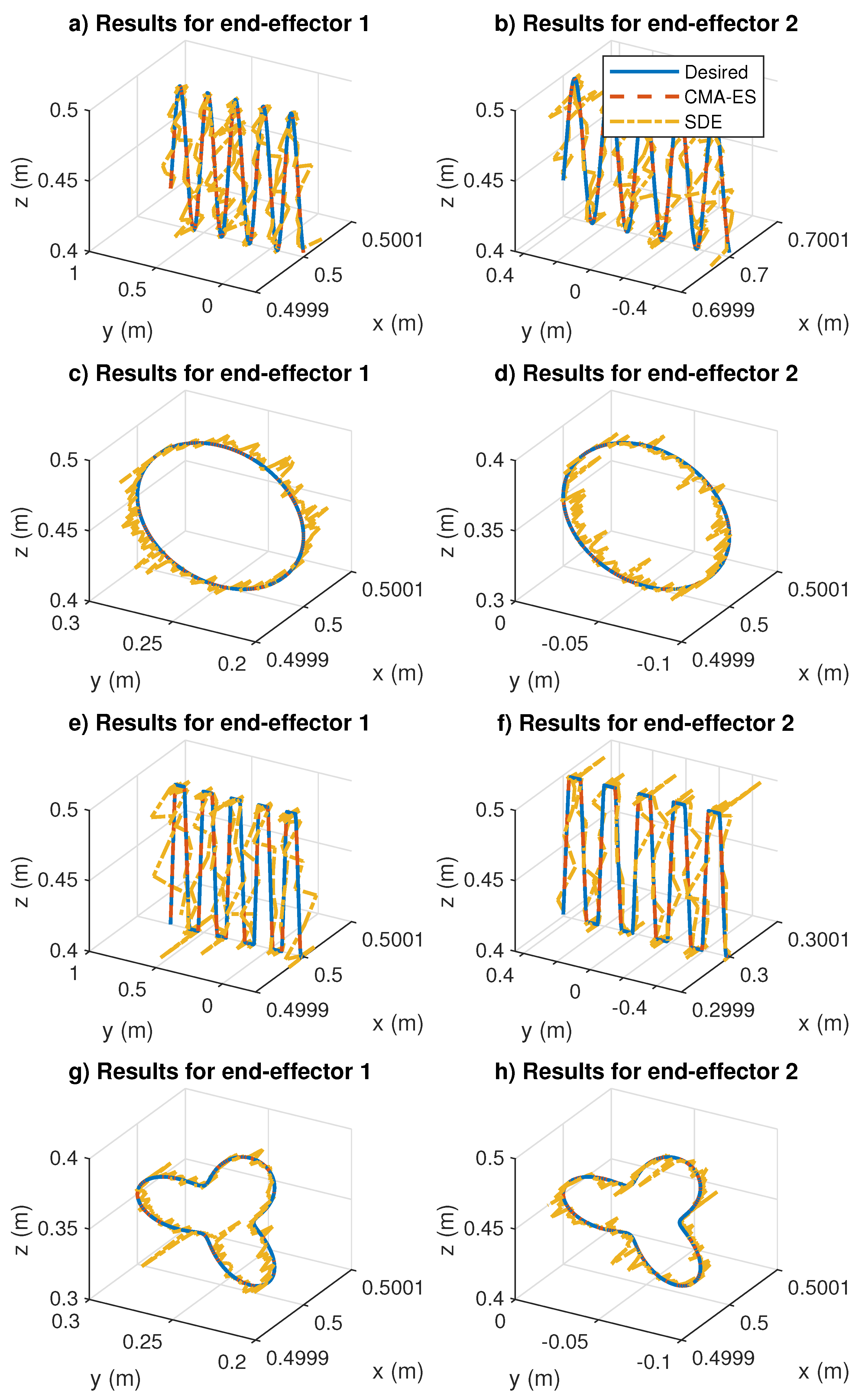
To visually see the differences in the position errors between CMA-ES and SDE, we considered including trajectory tracking graphs. The coordinated trajectory tracking results are provided in Figure 8. These results illustrate the successful trajectory tracking for all tests. As can be seen, the CMA-ES results fit perfectly in all given trajectories. Moreover, CMA-ES performed better than SDE. However, both algorithms provided excellent results.

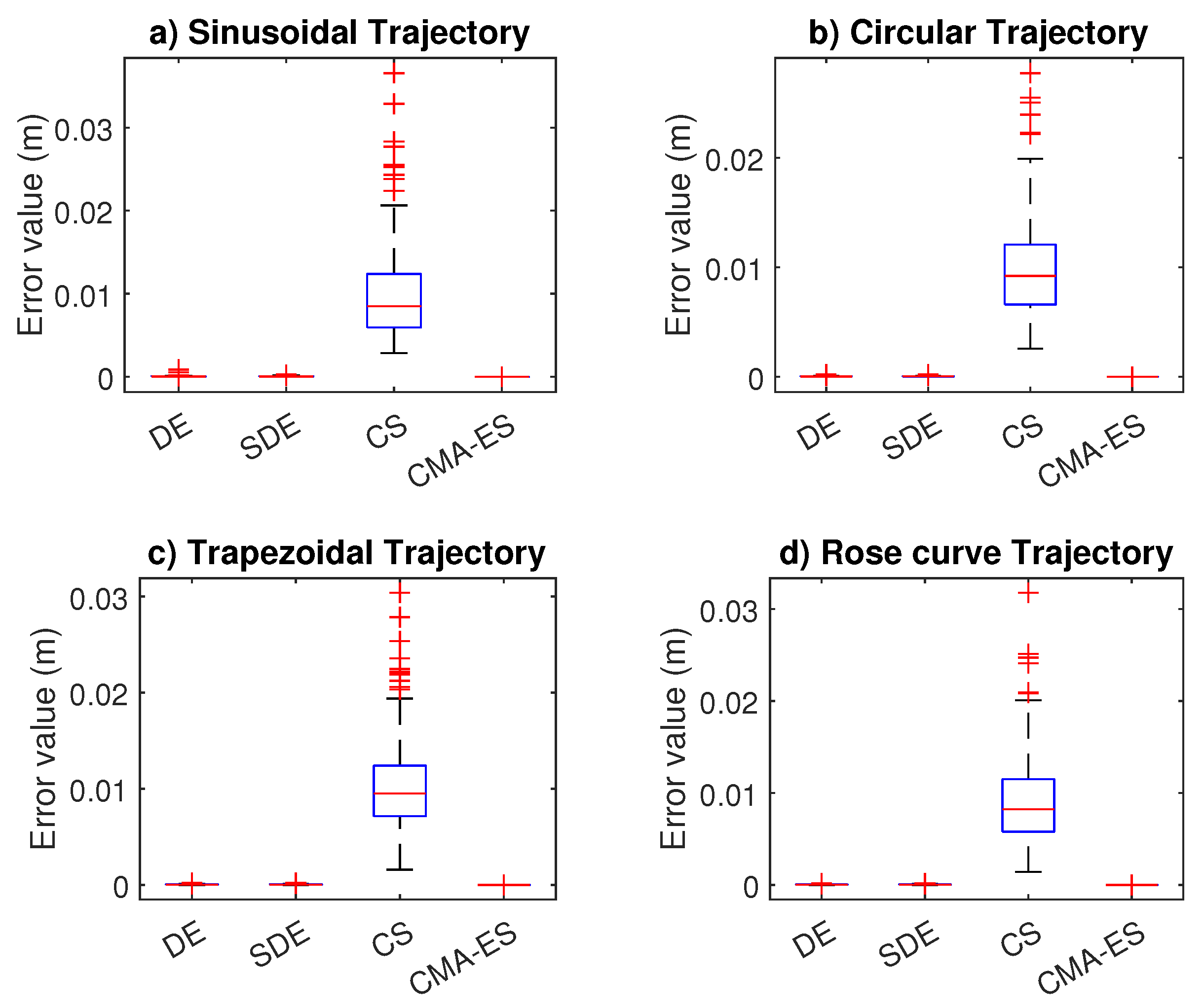
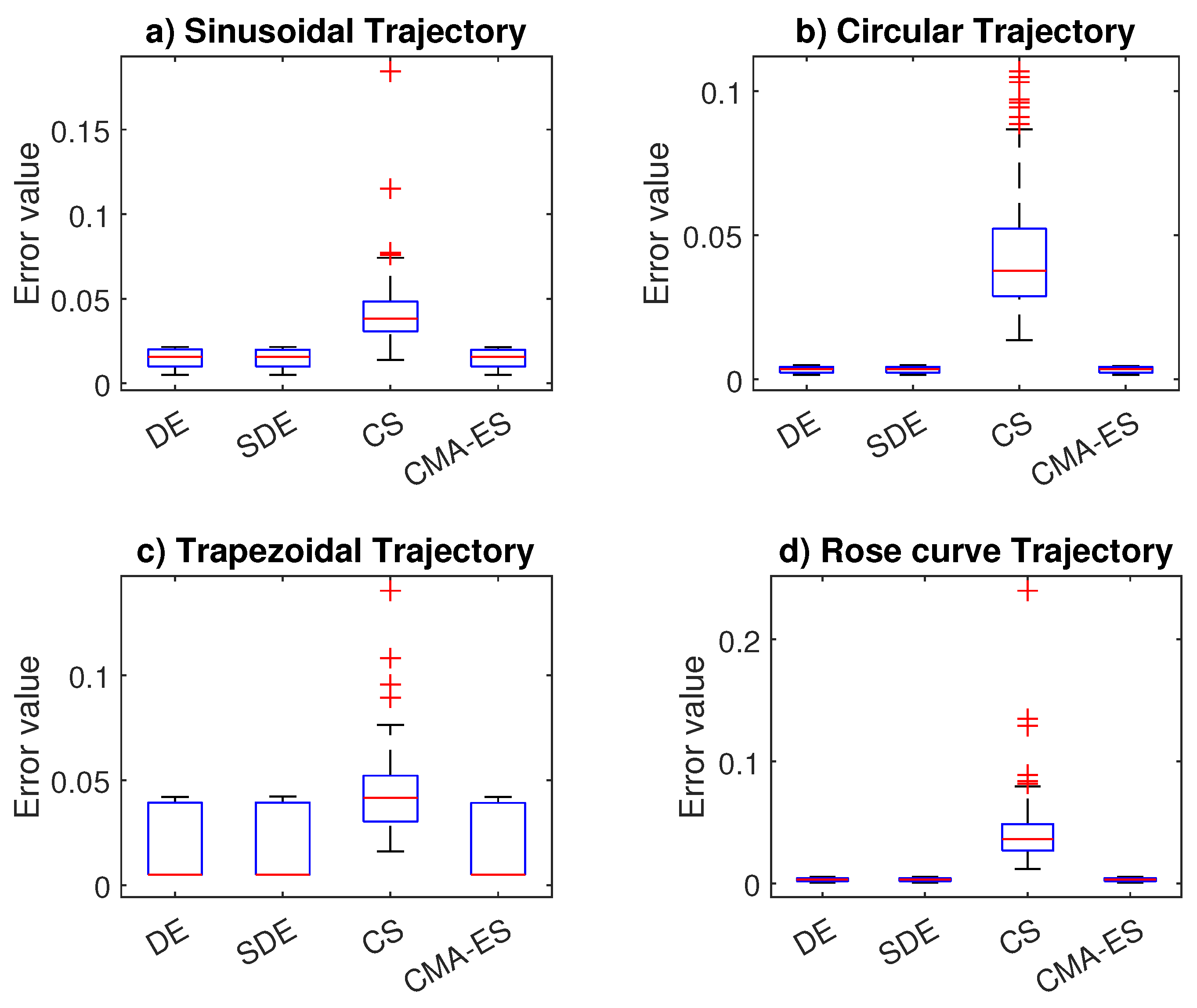
The motion error results from the coordinate trajectory tracking tasks are given in Figure 9. As expected, CS reported the worst results. It had the largest data dispersion with the presence of outliers in all tests. In contrast, DE, SDE, and CMA-ES performed similarly. Their data dispersion was small for the results in the sinusoidal, circular, and rose curve trajectories; see Figure 9a, Figure 9b, and Figure 9d, respectively. 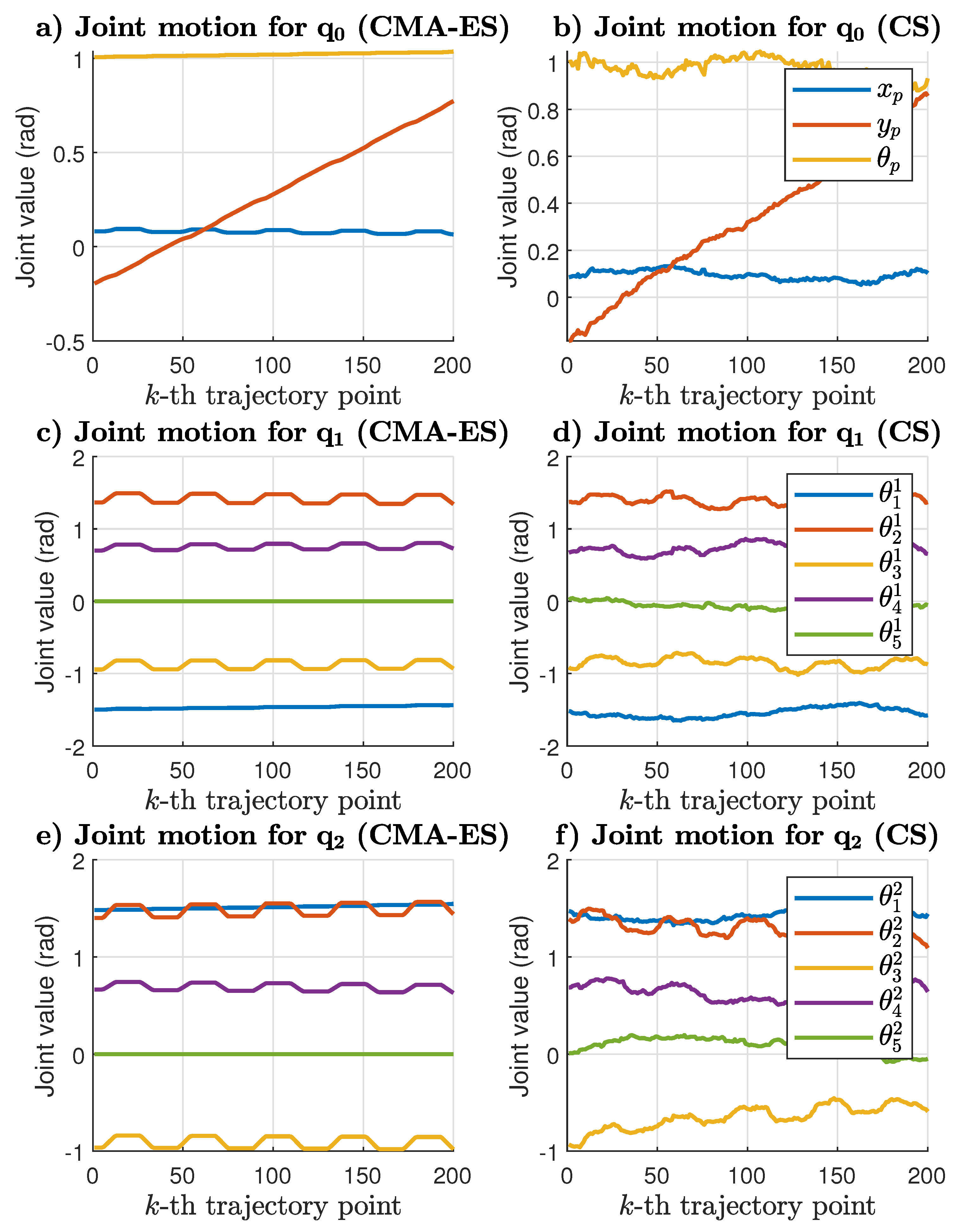Moreover, their results in Figure 9c indicated that the trapezoidal trajectory was more difficult to solve since more movement is required to follow the trajectory. Indeed, we considered including motion comparison graphs to analyze the performance of CMA-ES against CS for the trapezoidal trajectory. We did not consider including DE nor SDE for comparison because they performed similarly.

Figure 10 shows the motion results for the coordinate trapezoidal tracking. We compared the performance of CMA-ES against CS to emphasize the need for small motion errors. As we can see, CMA-ES showed smooth tracking results. In contrast, CS presented discontinuous motions. In real-world applications, it is important to avoid these rough motions since they can seriously damage and wear out the joints.

Based on the presented results, the CMAES algorithm was the most reliable method to solve coordinated trajectory tracking tasks. However, the DE and SDE algorithms are also recommended.

4.3. Real-World Experiments for Coordinated Trajectory Tracking

In this section, we are interested in presenting the applicability of the proposed approach in a real-world implementation. We propose to solve coordinated trajectory tracking based on the CMA-ES algorithm. The applicability was demonstrated using the KUKA^® Youbot^® system; see Figure 1.

The experiments were performed using the Robot Operating System (ROS) toolbox for Matlab. There exists an ROS component to access the KUKA^® Youbot^® hardware. This component provides a PID algorithm to control the joint positions of each manipulator. Moreover, this component also provides the current state of the joints based on encoder measures, and the current pose is given by odometry. To control the mobile platform pose, we used an adaptive PID scheme [35].

The coordinated trapezoidal trajectory task was considered for this test. The optimal solution found by CMA-ES represented a reference configuration ${\mathbf{q}}^{*}$. Indeed, we had a reference for the platform ${\mathbf{q}}_0^{*}$, a joint reference configuration for manipulator 1 ${\mathbf{q}}_1^{*}$, and a reference for manipulator 2 ${\mathbf{q}}_2^{*}$.

The presented results in this test were the comparative motion results between the reference and actual system configuration and the coordinated trajectory tracking results.

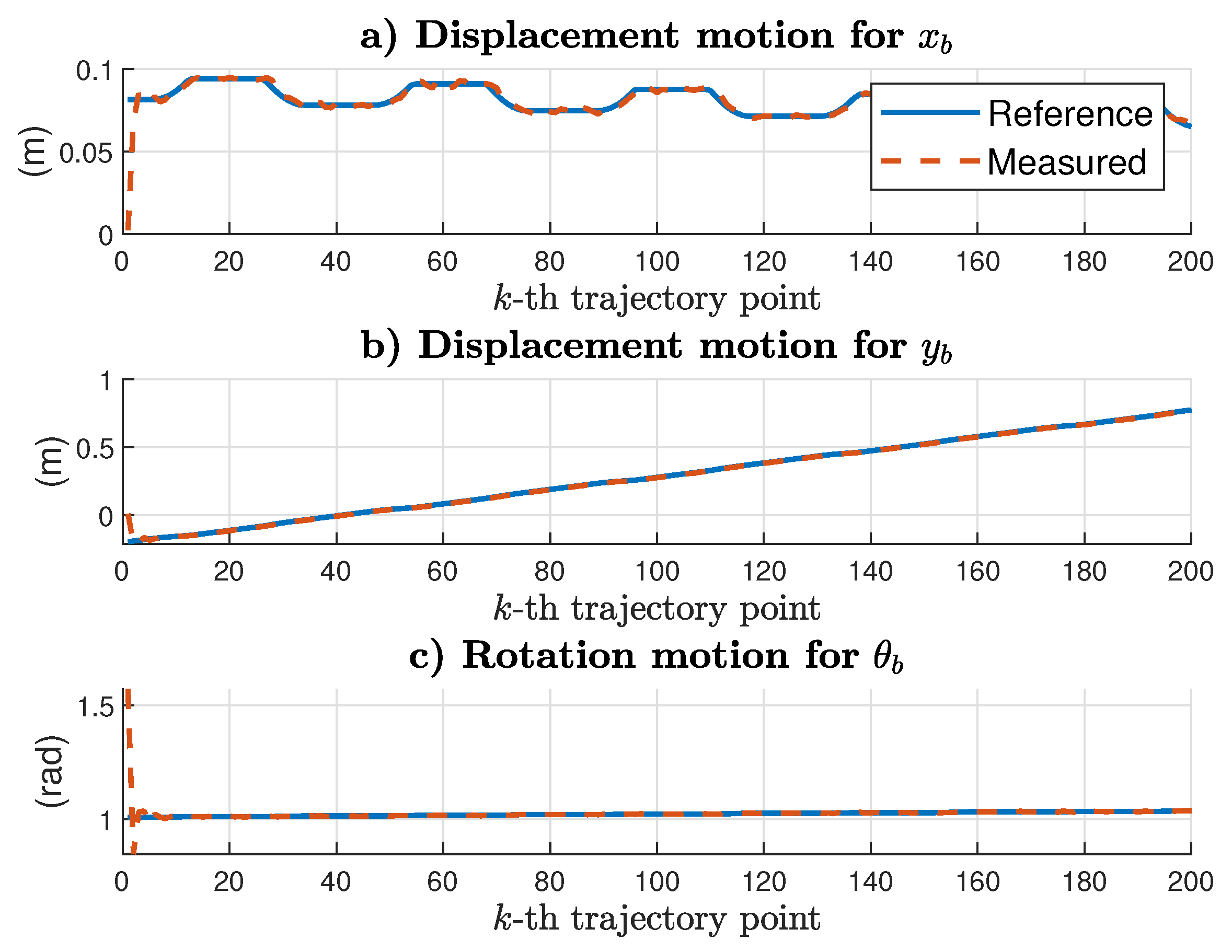
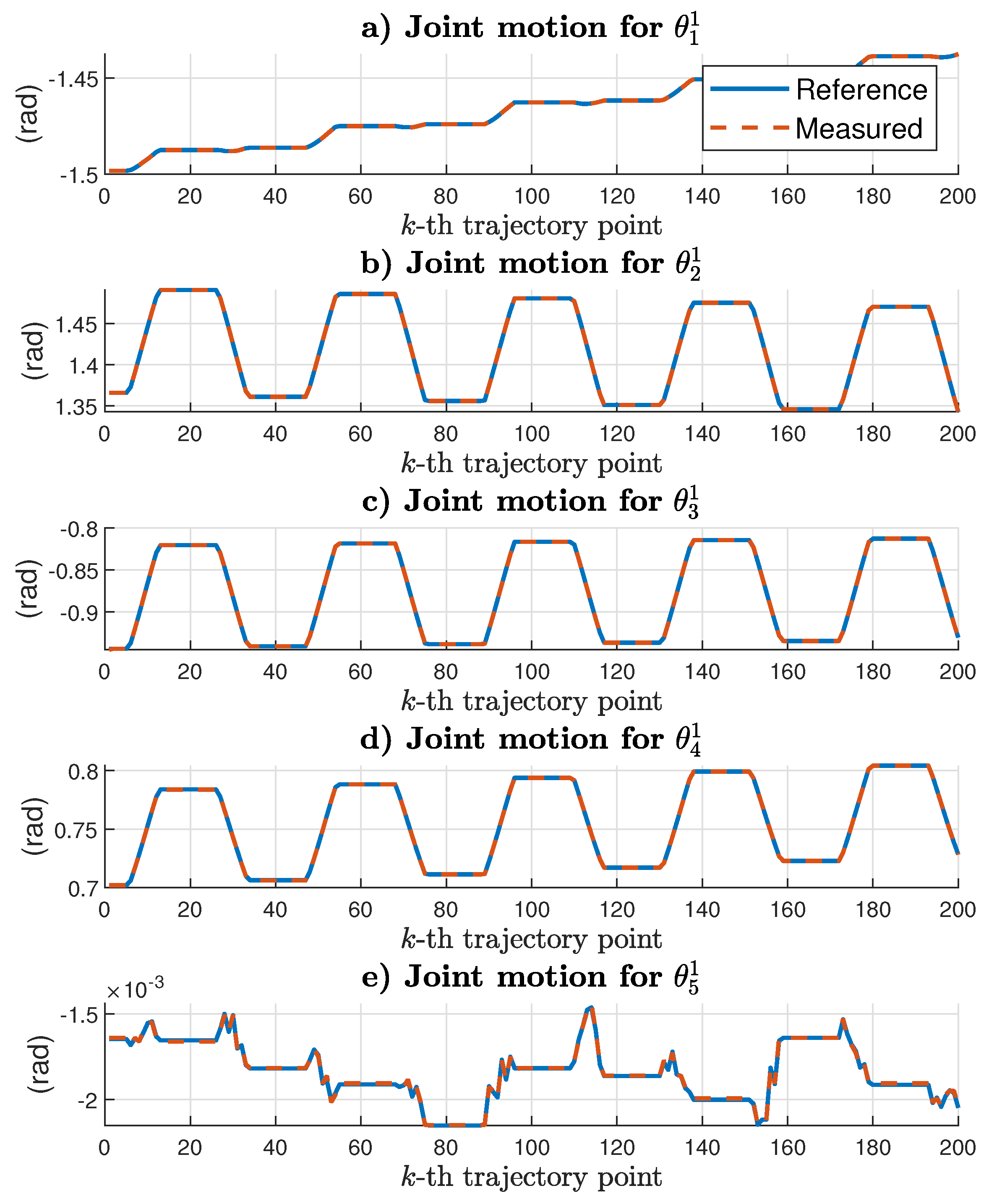
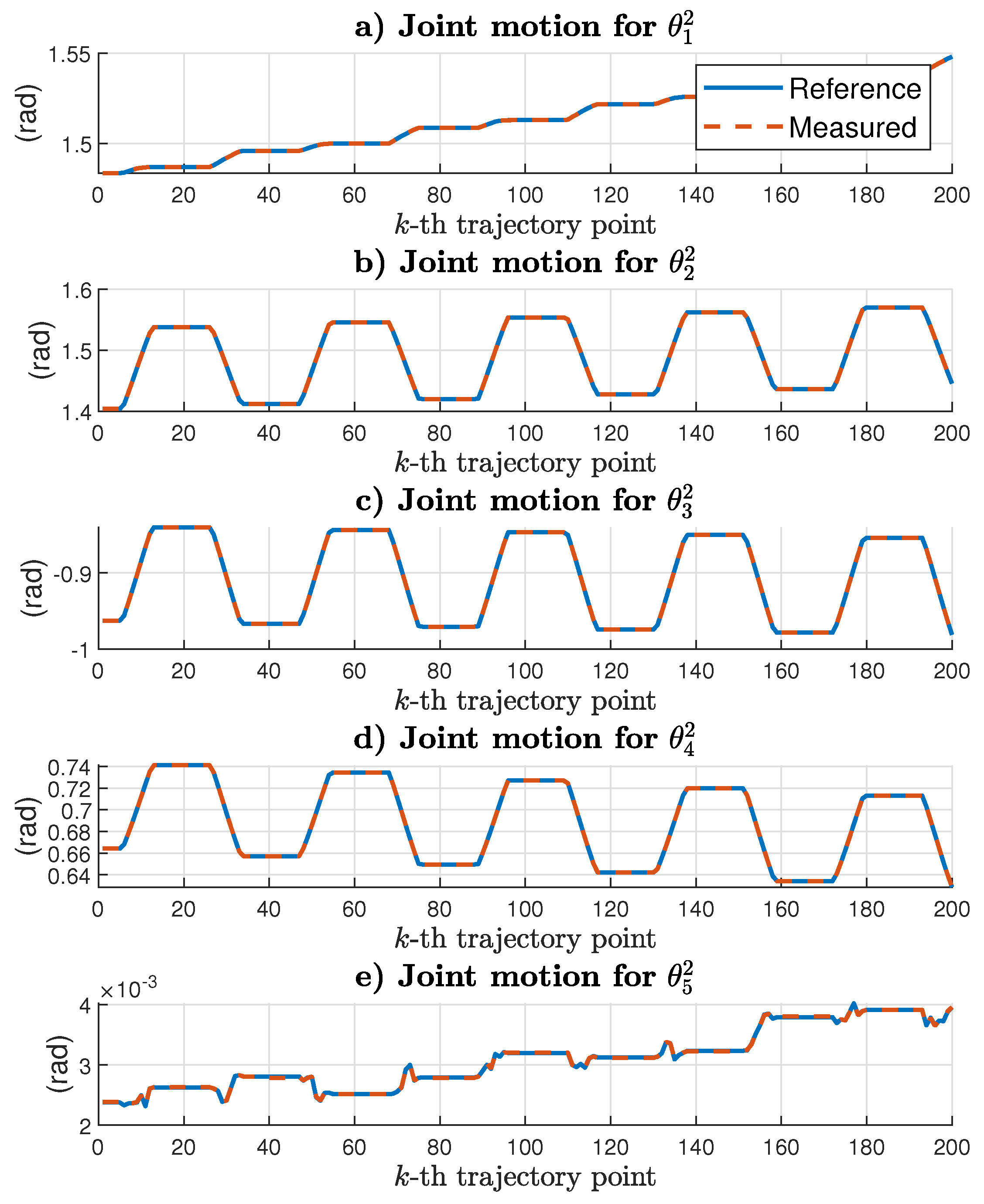
The motion control results for the mobile platform are given in Figure 11. Moreover, the motion control results for manipulator 1 and manipulator 2 are given in Figure 12 and Figure 13, respectively. For some of the first reference values, there was a greater following error. However, after the control laws reached the references, the following error was minimal. The reported results suggested that the reference and the actual values were practically the same. If the current system configuration were the same as the reference values, then the coordinate trajectory tracking should succeed.

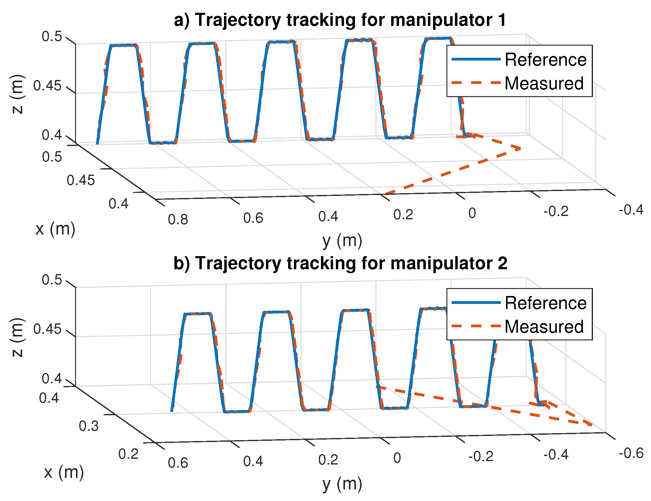
The coordinated trajectory tracking results are provided in Figure 14. As can be seen, both manipulators on board the same mobile platform succeeded in following the references as expected. We noticed that there were bigger tracking errors at the beginning of the trajectory, but this is normal since the actual position related to the initial system configuration was not close to the first reference point. When the control algorithm reached the reference, both trajectories were practically the same. We concluded that the coordinated trapezoidal tracking was successful.

5. Discussion

Gradient-based optimization algorithms are used to compute the minimum of a differentiable function. In the presence of multiple minima, these approaches may fail to find a global minimum. On the other hand, metaheuristics algorithms achieve global solutions, and the definition of the objective function does not necessarily have to be differentiable [36]. Metaheuristics algorithms are commonly used to solve the inverse kinematics of robotic manipulators. In this work, we proposed to solve the inverse kinematics of mobile dual-arm robots for coordinated manipulation. We considered including a comparative analysis among DE, CPABC, SDE, CS, QPSO, IMPSO, and CMA-ES to solve the inverse kinematics problems.

The comparative analyses indicated that CMA-ES outperformed the other algorithms with the highest accuracy and precise results. In the coordinated inverse kinematics tests, CMA-ES reported the smallest position error results with values below $1\times {10}^{-12}$ m. In the coordinated trajectory tracking tests, CMA-ES also reported the smallest position error results with values below $1\times {10}^{-8}$ m. In both tests, it also reported the smallest STD values and fastest convergence rates. Additionally, CMA-ES showed a minimal motion error, which is a smooth movement during trajectory tracking. For these reasons, we considered the CMA-ES algorithm the most reliable method for solving coordinated manipulation tasks.

The comparative analyses also indicated that DE and SDE stood out in both the coordinated inverse kinematics and coordinated trajectory tracking tests. Their performances were similar with position error values below $1\times {10}^{-5}$ m in both tests. Their STD values results were also remarkable. DE and SDE provided accurate and precise results with low movement errors.

The performance of CS was quite good in the coordinated inverse kinematics tasks, but its performance was poor in coordinated trajectory tracking. It seems that CS required more iterations to improve its performance. Moreover, the performance of CPABC, QPSO, and IMPSO was poor in both tests. The performance of these algorithms can be improved by carefully modifying their parameter settings. We concluded that these algorithms are not convenient to solve coordinated manipulation tasks.

Closed-form solutions give exact solutions for simple systems; for complex systems, they do not ensure a solution. In this case, the use of iterative methods is advised, which gives an approximate solution. The small position errors provided by the CMA-ES approach indicate highly precise results. It is important to note that such results are achieved in simulations. However, a position error of less than $1\times {10}^{-12}$ meters is difficult to achieve in real-world experiments due to hardware limitations. The use of industrial robots with the capability of high precision is required. Moreover, macro-robots are often used for medical proposes, which can achieve highly precise positions [37].

Although the proposed algorithm focuses on solving coordinate manipulation problems, this approach can also be applied to solve non-coordinated tasks. In non-coordinated manipulation, it is required to provide two independent inverse kinematics targets. The users need to provide the values of ${\mathbf{t}}_{{\mathsf{e}}_1}^{*}$ and ${\mathbf{t}}_{{\mathsf{e}}_2}^{*}$ independently. The rest of the inverse kinematics algorithm is practically the same.

This paper introduced a kinematic model for mobile dual-arm robots, using as the case of study the KUKA^® Youbot^® system. This system is composed of two 5-DOF manipulators attached to a 3-DOF omnidirectional platform. However, it is important to remark that the proposed scheme is not limited to this system; other manipulator configurations can be used to replace the ones used in this work. Since the forward kinematics is based on the DH model, no modifications to the inverse kinematics algorithm are required.

The proposed approach only considers the kinematic analysis to compute the mobile platform pose and the joint configuration of each arm to reach their desired end-effector position. Since the proposed approach is based on the forward kinematics equations, then the dynamical analysis is not required. Moreover, the optimal obtained configuration by the proposal was used as a reference for control purposes. Then, control strategies based on dynamic analysis can be used to control the system. Since the proposed approach computes the mobile and manipulators’ references, the control strategies can be implemented independently, with the advantage that the dynamic analysis of the complete system is not required.

To show the applicability of the proposed approach, real-world experiments were performed using the mobile dual-arm KUKA^® Youbot^® system to solve a coordinated trajectory tracking task. Moreover, we used a generic PID algorithm to control each manipulator’s joint position and an adaptive neuron PID to control the mobile platform pose. The reported results showed that the error references were close to zero, which implies that the cooperative task was successful.

Additional objectives in the optimization problems to solve the inverse kinematics of robotic manipulators have been proposed in recent years. Repulsive potential fields can be considered in the formulation of the objective function to deal with collision avoidance [38]. The use of the penalty function can also be used to handle joint limit constraints [29,30]. Moreover, the combination of metaheuristics algorithms and artificial neural networks provides the capacity to reduce time consumption [39,40]. Indeed, the use of recurrent neuronal networks is an appealing topic to deal with real-time inverse kinematics, and this has been proven to solve the control of redundant manipulators [41].

As a final remark, metaheuristics algorithms are often used for offline applications because they are time-consuming. However, the use of dedicated hardware such as the NVIDIA CUDA parallel architecture presents an interesting framework to significantly reduce time consumption, which is appealing for online and real-time applications [42].

6. Conclusions

This work introduced an approach for solving the inverse kinematics of mobile dual-arm robots for cooperative manipulation. Simulation and real-world experiments were performed to prove the effectiveness of the proposed approach for solving coordinated inverse and coordinated trajectory tracking tasks. Moreover, to solve the inverse kinematics, we used metaheuristics optimization algorithms. Then, comparative analyses were performed among the DE, CPABC, SDE, CS, QPSO, IMPSO, and CMA-ES algorithms. The experimental setup considered a mobile dual-arm system based on the KUKA^® Youbot^® system, which is composed of two 5-DOF manipulators attached to a 3-DOF omnidirectional platform.

Based on the comparative results, we can conclude that CMA-ES outperformed the other algorithms in all experiments. It reported the highest accuracy and precise results with the fastest convergence rates for coordinated inverse kinematics tasks. CMA-ES also provided the smoothest joint motions during coordinated trajectory tracking tasks. The performance of DE and SDE was also remarkable. They performed similarly in all tests with high accuracy and precision. They also provided smooth joint motions. CS performed better than CPABC, QPSO, and IMPSO in coordinated inverse kinematics tasks. However, it is not recommended for coordinated trajectory tracking due to its high motion errors. The CPABC, QPSO, and IMPSO algorithms are not recommended to solve the inverse kinematics of mobile dual-arm robots.

Additionally, the CMA-ES algorithm was tested for coordinated trajectory tracking in real-world experiments. The obtained optimal configurations were used as references. Then, ROS components were used to control the system. Since the references and the actual robot configuration perfectly matched, the results proved the applicability of the proposed approach.

Although the proposed approach focuses on solving coordinated inverse kinematics and coordinated trajectory tracking tasks, it can be implemented to solve non-coordinated manipulation as well. In future research, this work can be extended to solve the inverse kinematics of mobile dual-arm robots with non-holonomic platforms. Additionally, we propose to design a control scheme based on the dynamic model for the manipulator and the mobile platform to reach the references provided by the presented proposed approach.

The presented kinematic model considers an omnidirectional platform. It is appealing to propose an approach for mobile dual-arm robots with differential-drive or car-like platforms. However, the inverse kinematics approach must consider the non-holonomic constraints. We leave this approach for future research.