Article

Coupling Chemotaxis and Growth Poromechanics for the Modelling of Feather Primordia Patterning

1
Department of Mathematics, Università di Pavia, Via Ferrata 1, 27100 Pavia, Italy
2
Laboratory of Artificial & Natural Evolution (LANE), Department of Genetics and Evolution, University of Geneva, 30 Quai Ernest Ansermet, 1211 Geneva, Switzerland
3
SIB Swiss Institute of Bioinformatics, 1211 Geneva, Switzerland
4
School of Mathematics, Monash University, 9 Rainforest Walk, Melbourne, VIC 3800, Australia
5
Research Core on Natural and Exact Sciences, Universidad Adventista de Chile, Casilla 7-D, Chillán 3780000, Chile
*
Author to whom correspondence should be addressed.
Mathematics 2022, 10(21), 4096; https://doi.org/10.3390/math10214096
Submission received: 14 October 2022 / Revised: 28 October 2022 / Accepted: 28 October 2022 / Published: 3 November 2022
(This article belongs to the Special Issue Mathematical Modelling in Biomedicine III)

Abstract

:
In this paper we propose a new mathematical model for describing the complex interplay between skin cell populations with fibroblast growth factor and bone morphogenetic protein, occurring within deformable porous media describing feather primordia patterning. Tissue growth, in turn, modifies the transport of morphogens (described by reaction-diffusion equations) through diverse mechanisms such as advection from the solid velocity generated by mechanical stress, and mass supply. By performing an asymptotic linear stability analysis on the coupled poromechanical-chemotaxis system (assuming rheological properties of the skin cell aggregates that reside in the regime of infinitesimal strains and where the porous structure is fully saturated with interstitial fluid and encoding the coupling mechanisms through active stress) we obtain the conditions on the parameters—especially those encoding coupling mechanisms—under which the system will give rise to spatially heterogeneous solutions. We also extend the mechanical model to the case of incompressible poro-hyperelasticity and include the mechanisms of anisotropic solid growth and feedback by means of standard Lee decompositions of the tensor gradient of deformation. Because the model in question involves the coupling of several nonlinear PDEs, we cannot straightforwardly obtain closed-form solutions. We therefore design a suitable numerical method that employs backward Euler time discretisation, linearisation of the semidiscrete problem through Newton–Raphson’s method, a seven-field finite element formulation for the spatial discretisation, and we also advocate the construction and efficient implementation of tailored robust solvers. We present a few illustrative computational examples in 2D and 3D, briefly discussing different spatio-temporal patterns of growth factors as well as the associated solid response scenario depending on the specific poromechanical regime. Our findings confirm the theoretically predicted behaviour of spatio-temporal patterns, and the produced results reveal a qualitative agreement with respect to the expected experimental behaviour. We stress that the present study provides insight on several biomechanical properties of primordia patterning.

1. Introduction

Transport of species in tissue is a key process ubiquitous in biological systems. In particular, chemotaxis models [1] describe the directed movement of cells in response to chemicals (attractants or repellents), and can predict the formation of clustered structures. This mechanism has been observed in a variety of embryogenesis processes, such as gastrulation [2] and feather development [3]. In the latter, we refer to the buds that then give origin to feathers as primordia, and their origin has captured the attention of many theoretical and experimental studies. Mathematical models of different complexity have been used for primordia pattern formation, mainly based on the well-known Keller–Segel and Patlak–Keller–Segel-type chemotaxis equations considering fibroblast growth factor (FGF) and bone morphogenic protein (BMP) [4,5,6].
Poroelasticity refers to mixture models in which a solid phase coexists with (at least) one fluid phase/fluid particles [7]. In classical poroelastic structures composed by solid and fluid, the stress of the mixture is the sum of the interstitial pressure of the fluid and the stress of the (hyper)elastic solid phase, and both the fluid and solid phases are assumed to be incompressible. Biological organs and tissues are naturally porous at the tissue level, as they are heterogeneously composed, for example, of both muscle and blood, or of interstitial cerebrospinal fluid and cells, or collagen fibres and extracellular matrix in systems such as cartilage tissue. This phase separation persists even up to the cellular level, as there is the cytoskeleton and the cytoplasm. For this reason, poroelastic models have become very pervasive in the modelling of soft living tissue, such as in oedema formation [8,9], cardiac perfusion [10,11], lung characterisation [12], and brain injury [13].
In the context of biologically-oriented problems, experiments have shown that the rheology of cytoplasm within living cells exhibits a poroelastic behaviour [14], and in turn, the composition of cells and the extracellular matrix constitutes an overall poromechanical system. Using only fluid models lacks in general the possibility of producing heterogeneous proliferation patterns thanks to the stress localisation shear properties observed in deformable solids or solid-fluid mixtures. The presence of chemical solutes locally modifies morphoelastic properties and these processes can be homogenised to obtain macroscopic models of poroelasticity coupled with advection-reaction-diffusion equations (see e.g., [15,16]). In the proposed model we assume that the poroelastic growth tensor incorporates the contribution from the elongation of other structures in the skin such as collagen fibres. In this work we complement and extend the equations for feather primordia spatial organisation proposed by Painter et al. [6].
With this biological basis, the scope of our work is twofold: on one hand, we extend the existing pattern formation models for primordia, by considering their interaction with the intracellular space in the outset of growth. For this, in the regime of infinitesimal strains we incorporate an active stress in the solid phase which is regulated by morphogens. In the finite-strain regime we use a growth model which is consistent with the remodelling theory from, e.g., [17,18,19]. On the other hand, we perform a thorough stability analysis to understand the coupling mechanisms in the model and to investigate the conditions that give rise to pattern formation. The governing equations are of nonlinear nature, and they involve many vector and scalar fields. Attempting to solve them or to extract useful insight from their structure without further simplifications is very complicated. We first simplify and linearise the coupled system and carry out a thorough stability analysis based on non-trivial homogeneous steady states. We also derive appropriate base-case dispersion relations that serve to understand the coupling mechanisms in the proposed model, and they allow us to investigate the conditions that give rise to pattern formation. For this we follow the classical approach from, e.g., [13,20,21,22], where the so-called Routh–Hurwitz assumptions for stability are verified with the aim of further characterising relevant parametric spaces. These investigations allow us to conclude that an oscillatory Turing instability exists above a critical value of the mechanochemical coupling strength, for example.
It is important to mention that our paper also focuses on the numerical simulation of coupled chemotaxis-poromechanics models in 2D and 3D, which validate and extend the analytical results from the linear stability analysis. Many robust methods exist already for poroelasticity, see, e.g., [11,23,24,25,26,27] and the references therein. On the other hand, the theoretical numerical analysis of the properties of finite element discretisations for coupled poromechanics and two-species chemotaxis has been addressed in [28] using total pressure, and in [29] using conservative schemes; all these works focusing on the regime of linear poroelasticity. The modification of the analysis to accommodate the finite-strain framework has been recently conducted in [8,30]. Here we extend the latter formulations to include other morphogens and additional nonlinearities, and focus on a stronger two-way coupling required for the case of primordia patterns. The development of efficient preconditioners for chemotaxis has not yet been addressed in literature, whereas nonlinear poromechanics has already been studied [31,32] albeit only in a small deformations regime. In this work we provide efficient and scalable for both chemotaxis and large deformations poroelasticity.
We have structured the remainder of this paper in the following manner. Section 2 describes the coupled model for poro-mechano-chemical interactions, restricting the presentation to the regime of linear poroelasticity. We give an adimensional form of the governing equations, making precise boundary and initial conditions. In Section 3 we perform a linear stability analysis addressing pattern formation according to Turing instabilities. We separate the discussion in some relevant cases and derive and portray patterning spaces. Section 4 is devoted to extending the model to the case of nonlinear (finite-strain) poroelasticity and material growth, stating also the coupling with chemotaxis in the undeformed configuration. Some numerical examples are given in Section 5 and we close with a summary and discussion of model extensions and perspectives for future work in Section 6.

2. A Coupled Model of Linear Poroelasticity and Chemotaxis

Let us consider a piece of soft material as a porous medium in R d , d = 2 , 3 , composed by a mixture of incompressible grains and interstitial fluid, whose description can be placed in the context of the classical Biot consolidation problem (see e.g., [33]). In the absence of gravitational forces, of body loads, and of mass sources or sinks, we seek for each time t ( 0 , t final ] , the displacement of the porous skeleton, u ( t ) : Ω R d , and the pore pressure of the fluid, p ( t ) : Ω R , such that
t C 0 p + α B W div u 1 η div { κ p } = 0 in Ω × ( 0 , t final ] ,
σ = σ poroelast + σ act in Ω × ( 0 , t final ] ,
ρ t t u div σ = 0 in Ω × ( 0 , t final ] ,
where κ ( x ) is the hydraulic conductivity of the porous medium, ρ is the density of the solid material, η is the constant viscosity of the interstitial fluid, C 0 is the constrained specific storage coefficient, α B W is the Biot–Willis consolidation parameter. In (1b) we are supposing that the poromechanical deformations are also actively influenced by microscopic tension generation. A very simple description is given in terms of active stresses: we assume that the total Cauchy stress contains a passive and an active component, where
σ poroelast = λ ( div u ) I + 2 μ ε ( u ) α B W p I ,
and σ act is specified in (5), below. The tensor ε ( u ) = 1 2 ( u + u ) is that of infinitesimal strains, I denotes the second-order identity tensor, and  μ , λ are the Lamé constants (shear and dilation moduli) of the solid structure. Equations (1a)–(1c) represent the conservation of mass, the constitutive relation, and the conservation of linear momentum, respectively.
In addition, let us consider a modified Patlak–Keller–Segel model for the distribution of chemotactic cell populations of mesenchymal cells, m, epithelium activation state, e, fibroblast growth factor (FGF), f, and bone morphogenetic protein (BMP), b. The base-line model has been developed in [6] and (after being properly modified to account for the motion of the underlying deformable porous media) it can be summarised as follows
t m + t u · m div D m m α m exp ( γ m ) f = 0 in Ω × ( 0 , t final ] ,
t e [ κ 1 w ( x , t ) h 1 ( m ) + κ 2 h 2 ( m ) ] ( 1 e ) + [ 1 h 1 ( m ) ] ( κ 3 + κ 4 b ) e = 0 in Ω × ( 0 , t final ] ,
t f + t u · f div ( D f f ) κ F e + δ F f + ξ f div u = 0 in Ω × ( 0 , t final ] ,
t b + t u · b div ( D b b ) κ B h 3 ( m ) m + δ B b = 0 in Ω × ( 0 , t final ] ,
where D m , D f , D b are positive definite diffusion matrices, and the spatio-temporal and nonlinear coefficients (in this case, the priming wave responsible for the generation of spatial patterns and the degree of clustering of mesenchymal cells, respectively) are defined as
w ( x , t ) = ω 1 2 { 1 + tanh ( ω 2 [ t x 2 / ω 3 ] ) } , h i ( m ) = m P i [ K i P i + m P i ] 1 ,
where κ i , ω i , P i , γ , δ i , ξ f are positive model constants. Note that the mechano-chemical feedback (the process where mechanical forces modify the reaction-diffusion effects) is here assumed only through an additional reaction term in the FGF Equation (3c), depending linearly on volume change. Since ξ f > 0 , this contribution acts as a local sink of FGF during dilation.
On the other hand, we assume that the active stress component acts isotropically on the medium (see e.g., [17]), and it depends nonlinearly on the concentration of mesenchymal cells, as proposed for instance in [21]
σ act = λ + 2 μ 3 τ m 1 + ζ m 2 I ,
with τ a model constant to be specified later on, which can be positive (implying that the function modifies the motion of the medium as a local dilation) or negative (isotropically distributed compression).
In order to reduce the number of model parameters, we focus on a dimensionless counterpart of systems (1a)–(1c) and (3a)–(3d), which can be derived using the following transformation, suggested in [6]
m = m * γ , e = e * , f = κ F f * δ B , b = κ B b * γ , u = D b δ B u * , p = p * , t = t * δ B , x = D b δ B x * ,
where hereafter the stars are dropped for notational convenience. The adimensional coupled system is then equipped with appropriate initial data at rest
m ( 0 ) = m 0 , e ( 0 ) = e 0 = κ 1 w ( x , 0 ) h 1 ( m 0 ) + κ 2 h 2 ( m 0 ) κ 1 w ( x , 0 ) h 1 ( m 0 ) + κ 2 h 2 ( m 0 ) + [ 1 h 1 ( m 0 ) ] ( κ 3 + κ 4 b ) , f ( 0 ) = e 0 δ F , b ( 0 ) = h 3 ( m 0 ) m 0 , u ( 0 ) = 0 , t u ( 0 ) = 0 , p ( 0 ) = 0 ,
defined in Ω ; and boundary conditions in the following manner
{ D m m α m exp ( γ m ) f } · n = D f f · n = b · n = 0 on Ω × ( 0 , t final ] ,
u = u Γ and κ η p · n = 0 on Γ × ( 0 , t final ] ,
σ = t and p = p 0 on Σ × ( 0 , t final ] ,
where denotes the outward unit normal on the boundary, and  Ω = Γ Σ is disjointly split into Γ and Σ where we prescribe clamped boundaries and zero fluid normal fluxes; and a given traction t together with constant fluid pressure p 0 , respectively.

3. Linear Stability Analysis and Dispersion Relation

3.1. Preliminaries

We proceed to derive a linear stability analysis for the coupled problem (1a)–(5). As usual the analysis is performed on an infinite domain in R d , with  d = 2 , 3 . The first step consists in linearising the poro-mechano-chemical system around a steady state, defined in (6). The linearised dimensionless equations are given by
t C 0 p + α B W div u 1 η div { κ p } = 0 , ρ t t u div σ poroelast + σ act lin = 0 , t m div { D m m α m 0 e m 0 f } = 0 , t e A m ( m 0 , e 0 ) m + A e ( m 0 , b 0 ) e + A b ( m 0 , e 0 ) b = 0 , t f div { D f f } e + δ F f + ξ f div u = 0 , t b Δ b H 3 ( m 0 ) m + δ B b = 0 ,
where
σ act lin = λ + 2 μ 3 τ 1 ζ m 0 2 1 + ζ m 0 2 2 m I ,
and A m , A e , A b , H 3 are functions of the steady state values, which will be made precise in Definition 1, below. We look then for solutions of the form u , p , m , e , f , b e i k · x + ϕ t , where k is the wave vector (a measure of spatial structure) and ϕ is the linear growth factor. By substituting this ansatz on the system (8), we get a system of linear equations for the vector w = u , p , m , e , f , b , where the associated complex eigenvalues ϕ , give information on occurrence of instability of the steady state (i.e., pattern formation), when its real component is positive. It is worth pointing out that the present analysis will only address Turing patterning (Hopf bifurcations or other forms of instability that relate to analysing the imaginary part of ϕ , are not considered). In order to specify the aforementioned system of equations for w , we collect in Proposition 1 some useful preliminary relations. The proof is postponed to the Appendix A.
 Proposition 1. 
Let g, v be sufficiently regular scalar and vector functions defined by g = exp ( i k · x + ϕ t ) and v = v 0 exp ( i k · x + ϕ t ) (with v 0 , a constant vector), respectively. Let us also set θ = div v . Then
f = i k f , Δ f = i 2 f k · k = k 2 f , t f = ϕ f , v = i v k , div v = i v · k , t v = ϕ v ,
div ε ( v ) = ( v · k ) k + k 2 v 2 , t ε ( v ) = ϕ ε ( v ) , div ( θ I ) = ( v · k ) k , t θ = ϕ θ .
The sought system is defined next, starting from (8).
 Definition 1. 
Let w = u , p , m , e , f , b R d + 5 , d = 2 , 3 be the vector of independent variables. Then the associated linear system is given by M w = 0 d + 5 , where the matrix M ( d + 5 ) × ( d + 5 ) adopts the form
M = M 11 M 12 M 21 M 22 ,
with the blocks defined as
M 11 = A 1 k 1 + B A 1 k 2 A 1 k d i k 1 A 2 k 1 A 2 k 2 + B A 2 k d i k 2 A d k 1 A 1 k 2 A d k d + B i k d i α B W ϕ k 1 i α B W ϕ k 2 i α B W ϕ k d C , M 12 = i λ + 2 μ 3 τ 1 ζ m 0 2 1 + ζ m 0 2 2 k 1 0 0 0 i λ + 2 μ 3 τ 1 ζ m 0 2 1 + ζ m 0 2 2 k d 0 0 0 , M 21 = 0 0 0 0 i ξ f k 1 i ξ f k d 0 0 , M 22 = ϕ + D m k 2 0 α m 0 e m 0 k 2 0 A m ϕ + A e 0 A b 0 1 ϕ + D f k 2 + δ F 0 H 3 0 0 ϕ + k 2 + 1 ,
and where the relevant entries are defined as B = ρ ϕ 2 + μ k 2 , C = C 0 ϕ + κ η k 2 , and 
A i = μ + λ k i , for all i in { 1 , , d } , A m = κ 1 ω 1 h 1 ( m 0 ) + κ 2 h 2 ( m 0 ) ( 1 e 0 ) + h 1 ( m 0 ) ( κ 3 + κ 4 b 0 ) e 0 , A e = κ 1 ω 1 h 1 ( m 0 ) + κ 2 h 2 ( m 0 ) + ( 1 h 1 ( m 0 ) ) ( κ 3 + κ 4 b 0 ) , A b = ( 1 h 1 ( m 0 ) ) κ 4 e 0 , H 3 = h 3 ( m 0 ) + h 3 ( m 0 ) m 0 .
We then proceed to obtain a dispersion relation associated with the characteristic polynomial P ( ϕ ) = det ( M ) of the matrix described in Definition 1. We obtain
P ( ϕ ; k 2 ) = B ( ϕ ; k 2 ) d 1 P 1 ( ϕ ; k 2 ) + P 2 ( ϕ ; k 2 ) P 3 ( ϕ ; k 2 ) ,
where B ( ϕ ; k 2 ) = ρ ϕ 2 + μ k 2 is a polynomial with pure imaginary roots. Consequently, it does not have an influence on the stability of the steady state of system (1a)–(5). The polynomials P i , i = 1 , 2 , 3 , are given in what follows.
 Definition 2. 
The polynomials conforming the characteristic Equation (10) are
P 1 ( ϕ ; k 2 ) = b 3 ϕ 3 + b 2 ϕ 2 + b 1 ϕ + b 0 , P 2 ( ϕ ; k 2 ) = a 4 ϕ 4 + a 3 ϕ 3 + a 2 ϕ 2 + a 1 ϕ + a 0 , P 3 ( ϕ ; k 2 ) = c 3 ϕ 3 + c 2 ϕ 2 + c 1 ϕ + c 0 ,
where all coefficients in (11) adopt the following forms
a 0 = D m D f ( k on + k off ) k 6 + ( D m δ B + D m D f ) ( k on + k off ) α m 0 e m 0 A m k 4 + D m δ B ( k on + k off ) + α m 0 e m 0 H 3 A b α m 0 e m 0 A m k 2 , a 1 = D m D f k 6 + ( D m D f + D m + D f ) ( k on + k off ) + D m δ B + D m D f k 4 + ( D m δ B + δ B + D m + D f ) ( k on + k off ) + D m δ B α m 0 e m 0 A m k 2 + δ B ( k on + k off ) , a 2 = D m D f + D m + D f k 4 + D m δ B + ( D m + D f + 1 ) ( k on + k off ) + δ + D m + D f k 2 + ( δ B + 1 ) ( k on + k off ) + δ B , a 3 = D m + D f + 1 k 2 + δ B + k on + k off + 1 , a 4 = 1 , b i = ξ f λ + 2 μ 3 τ 1 ζ m 0 2 1 + ζ m 0 2 2 α m 0 e m 0 k 2 b ^ i , b ^ 0 = κ η k on + k off k 2 + 1 k 2 , b ^ 1 = κ η k 4 + C 0 + κ η k on + k off + κ η k 2 + C 0 k on + k off , b ^ 2 = C 0 + κ η k 2 + C 0 k on + k off + 1 , b ^ 3 = C 0 , c 0 = κ η ( 2 μ + λ ) k 4 , c 1 = C 0 ( 2 μ + λ ) + α B W k 2 , c 2 = ρ κ η k 2 , c 3 = ρ C 0 , k on = κ 1 ω 1 h 1 ( m 0 ) + κ 2 h 2 ( m 0 ) , k off = ( 1 h 1 ( m 0 ) ) ( κ 3 + κ 4 b 0 ) .
From Definition 2 we immediately see that the characteristic polynomial is of up to seventh degree, making it difficult to determine analytically the main features of the system.
Next we concentrate on addressing some specific scenarios of particular interest. Unless specified otherwise, we will employ the parameter values provided in Box 1. Note that the term σ act lin vanishes for m 0 = 1 , so, differently from [6], we modify the steady state for mesenchymal cells concentration to m 0 = 2 .
Box 1. Model parameters used in the linear stability analysis of the poro-mechano-chemical system
m 0 = 2 , D m = 0.01 , D f = 0.1 , α = 4 , κ 1 = 0.05 , κ 2 = 0.025 , κ 3 = 1 , κ 4 = 1 ,
K 1 = 1 , K 2 = 2 , K 3 = 5 , P 1 = P 2 = P 3 = 2 , δ F = 1 , ω 1 = 1 , ω 2 = 5 , ω 3 = 0.04
E = 3 · 10 4 , ν = 0.4 , C 0 = 10 3 , κ = 10 4 , α B W = 0.1 , τ = 60 , η = 0.1 , ξ f = 0.15 , ρ = 1 , ζ = 1

3.2. Spatially Homogeneous Distributions

If k 2 = 0 then the characteristic polynomial P ( ϕ ; k 2 ) is
P ( ϕ ; 0 ) = ρ C 0 ϕ 8 [ ϕ 3 + δ B + k on + k off + 1 ϕ 2 + ( δ B + 1 ) ( k on + k off ) + δ B ϕ + δ ( k on + k off ) ] .
The well-known Routh–Hurwitz conditions (see e.g., [34]) state that for any polynomial of order 3, a necessary and sufficient set of conditions should be satisfied in order to ensure that all the roots are in the space of complex non-positive real values, C = { z C : ( z ) 0 } . For a general polynomial P ( ϕ ) = α 3 ϕ 3 + α 2 ϕ 2 + α 1 ϕ + α 0 , where all the α i > 0 , we have
α 2 α 1 α 3 α 0 > 0 .
In our case, α 2 α 1 α 3 α 0 = ( δ B + 1 ) ( k on + k off ) + δ B δ B + k on + k off + δ B + k on + k off , which is a real positive constant. This indicates that the steady state is stable in a spatially homogeneous system, irrespective of the value of the model parameters.

3.3. Zero Chemotaxis

When α = 0 , all the coefficients b i from Definition 2 are zero. Consequently, the characteristic polynomial is defined by the sub-polynomials P 2 and P 3 only. As all the parameters implied in c i are positive and the Routh–Hurwitz condition (12) is satisfied, we know that the P 3 polynomial has only non-positive real part complex solutions and therefore does not influence the stability of the steady state. Thus, the instability condition can only come from P 2 , related only to the chemotaxis model analysed in [6]. Substituting α = 0 in the sub-matrix M 22 leads to a dispersion relation
P ( ϕ ) = ( ϕ + D m k 2 ) ( ϕ + A e ) ( ϕ + D f k 2 + δ F ) ( ϕ + k 2 + 1 ) ,
and consequently the roots are negative real numbers. The absence of chemotaxis prevents then any pattern formation irrespective of the presence or absence of poro-mechanical coupling.

3.4. Uncoupled System

Similarly as in the no-chemotaxis scenario above, imposing τ = 0 or ξ f = 0 leads to P 1 ( ϕ ; k 2 ) = 0 for all ϕ , k 2 . Additionally, as  P 3 ( ϕ ; k 2 ) has only non-positive roots, only the chemotaxis sub-polynomial enables us to find eigenvalues that lead to unstable systems. For  P 2 the Routh–Hurwitz conditions are given by
a i > 0 , a 2 a 3 a 1 a 4 > 0 and a 1 a 2 a 3 a 0 a 3 2 a 1 2 a 4 > 0 .
Then, from Definition 2, we can readily observe that a 4 , a 3 and a 2 are real positive coefficients for any positive parameter value. A complete analysis of (13) is analytically quite involved. Nevertheless, and in accordance with the analysis in [6], we can restrict the discussion to the conditions that break a 0 > 0 .
We first observe, from its definition, that a 0 is a polynomial of even order with respect to k 2 , guaranteeing that it has at least one local extrema. Consequently, we look for the critical wave number, k c 2 > 0 , defined by the equation a 0 ( k 2 ) = 0 , that substituting in a 0 will lead exactly to be at zero for the associated critical parameter θ c that we want to analyse (i.e.,  a 0 ( θ c ; k c 2 ) = 0 ). In the uncoupled scenario, a 0 is a quadratic polynomial with respect to k 2 and roots can be easily obtained. Nonetheless, in order to have a 0 negative for positive k 2 , one has to satisfy the following three conditions
( D m δ B + D m D f ) ( k on + k off ) α m 0 e m 0 A m < 0 ,
D m δ B ( k on + k off ) + α m 0 e m 0 H 3 A b α m 0 e m 0 A m < 0 , 4 ( D m δ B + D m D f ) ( k on + k off ) α m 0 e m 0 A m 2
12 D m D f ( k on + k off ) D m δ B ( k on + k off ) + α m 0 e m 0 H 3 A b α m 0 e m 0 A m > 0 .
Either (14a) or (14b) enforces that k 2 has a real positive part, while (14c) is necessary to have a real wave number. These conditions are similar to the ones stated in [6]. The inequality (14b) emphasises how the positive feedback mechanism of the accumulation of mesenchymal cells through chemotaxis leads to stimulate further FGF secretion, based on the activation of the epithelium. When the condition is satisfied, patterning is achieved.
Condition (14a) indicates that the steady state is destabilised when A m > 0 , occurring when the clustering-mediated activation is sufficiently strong. Figure 1 (panels (A1)–(B1)) present the patterning space based on the implicit functions defined in (14a)–(14c) for the ( m 0 , α ) and ( κ 1 , κ 4 ) space. The conditions are represented in both Figures by a plain-green curve (14a), a red-dot-dashed curve (14b), and a blue-dashed curve (14c). The boundaries present very similar results to the linear analysis from [6]. Here, we accentuate the region by filling it with light grey. Panels (A2)–(A3) and (B2)–(B3) in Figure 1 portray the functions a 0 ( k 2 ) (parameter condition) and λ ( k 2 ) (dispersion relation) for the studied parameters m 0 and κ 4 . We present in different colours the behaviour of the system for the critical parameter value (green curve), as well as parameter values obtained by increasing and decreasing by 25% and 50% the critical value, where we recall that fixed parameters are taken from Box 1. We see that moving above or below the critical value results in a finite interval of wave numbers for which the complex eigenvalue presented positive real component and thus leading to instability (patterning). As illustrated also in [6], for a specific parameter set, panels (A1)–(A3) from Figure 1 show that a sufficiently dense dermis cells concentration is necessary to produce instability. While increasing the chemotaxis sensibility of the system we spread the range of possible mesenchymal cells density, by the u-shape form of the boundary, a sufficiently high density of cells can prevent pattern formation (see Figure 1(A1)). The capacity of BMP to deactivate the epithelium by increasing κ 4 , rapidly decreases the patterning ability of the system.

3.5. Zero Activation/Inactivation of Epithelium

Different scenarios are possible in such case: only zero activation ( κ 1 = κ 2 = 0 , e 0 = 0 ), only zero inactivation ( κ 3 = κ 4 = 0 , e 0 = 1 ) or both zero activation and inactivation of the epithelium. Contrary to [6], the coupling with the poroelastic structure leads to a more involved analysis of the system and, in particular, it does not guarantee emerging patterns. In any case, the coefficients A m and A b will be zero and bring the coefficients of P 2 to be strictly positive. As the coefficients of P 3 are also non-negative, P ( ϕ ; k 2 ) can only lead to negative eigenvalues if the coefficients of P 1 are negative. By Definition 2, we know that the b i ’s are negative only if the coupled-dependent constant is itself negative, and this phenomenon occurs if one of the following conditions is satisfied
λ + 2 μ 3 τ 1 ζ m 0 2 1 + ζ m 0 2 2 > 0 { τ > 0 and m 0 < 1 ζ τ < 0 and m 0 > 1 ζ .
If one of the condition is satisfied, the formation of patterns is expected. This is an opposite conclusion as that drawn in the case of chemotaxis only [6].

3.6. General Case

The thorough analysis of the coupled system involves a seventh-order polynomial. Analytical Routh–Hurwitz conditions in this case are hardly accessible and the crossed effects due to multiple parameters and conditions will inevitably make difficult the interpretation of the system behaviour. We can however restrict then the analysis to ϕ 0 , with coefficients d 0 = a 0 c 0 + b 0 , where a 0 , b 0 , c 0 are as in Definition 2. After some algebraic manipulations, we derive d 0 with respect to k 2 and obtain
d 0 ( k 2 ) = θ 4 k 8 + θ 3 k 6 + θ 2 k 4 + θ 1 k 2 ,
where
θ 1 = 2 ξ f λ + 2 μ 3 τ 1 ζ m 0 2 1 + ζ m 0 2 2 α m 0 e m 0 ( k on + k off ) , θ 2 = 3 [ ( 2 μ + λ ) D m δ B ( k on + k off ) + α m 0 e m 0 H 3 A b α m 0 e m 0 A m ξ f λ + 2 μ 3 τ 1 ζ m 0 2 1 + ζ m 0 2 2 α m 0 e m 0 ( k on + k off ) ] , θ 3 = 4 ( 2 μ + λ ) ( D m δ B + D m D f ) ( k on + k off ) α m 0 e m 0 A m , θ 4 = 5 D m D f ( 2 μ + λ ) ( k on + k off ) .
In contrast with the uncoupled case studied above, here k c 2 is found by solving a quartic polynomial (employing the intrinsic MATLAB function roots, after constructing the associated vector of polynomial coefficients). In addition, one needs to satisfy some additional conditions leading to d 0 < 0 for any positive k 2 . More specifically, the constraints consist of at least one of the Routh–Hurwitz conditions [34], stated as
θ 1 > 0 , θ 2 > 0 , θ 3 > 0 ,
θ 2 θ 3 θ 1 θ 4 > 0 ,
θ 1 θ 2 θ 3 θ 1 2 θ 4 > 0 ,
or the discriminant
27 θ 4 2 θ 1 4 + 18 θ 4 θ 3 θ 2 θ 1 3 4 θ 4 θ 2 3 θ 1 3 4 θ 3 3 θ 1 3 + θ 3 2 θ 2 2 θ 1 2 > 0 .
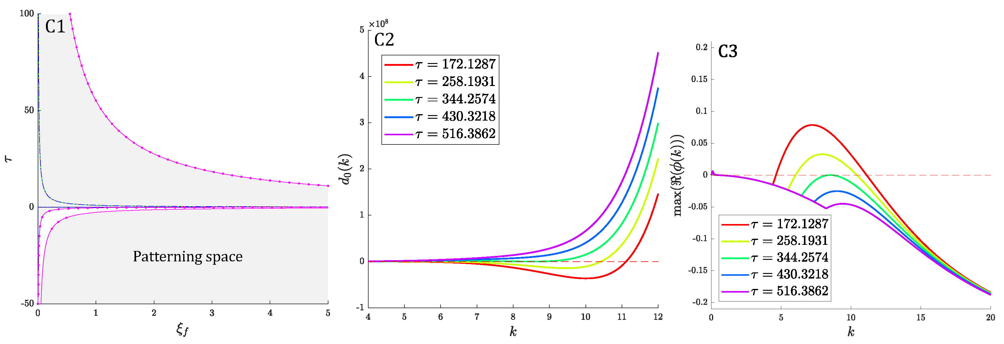
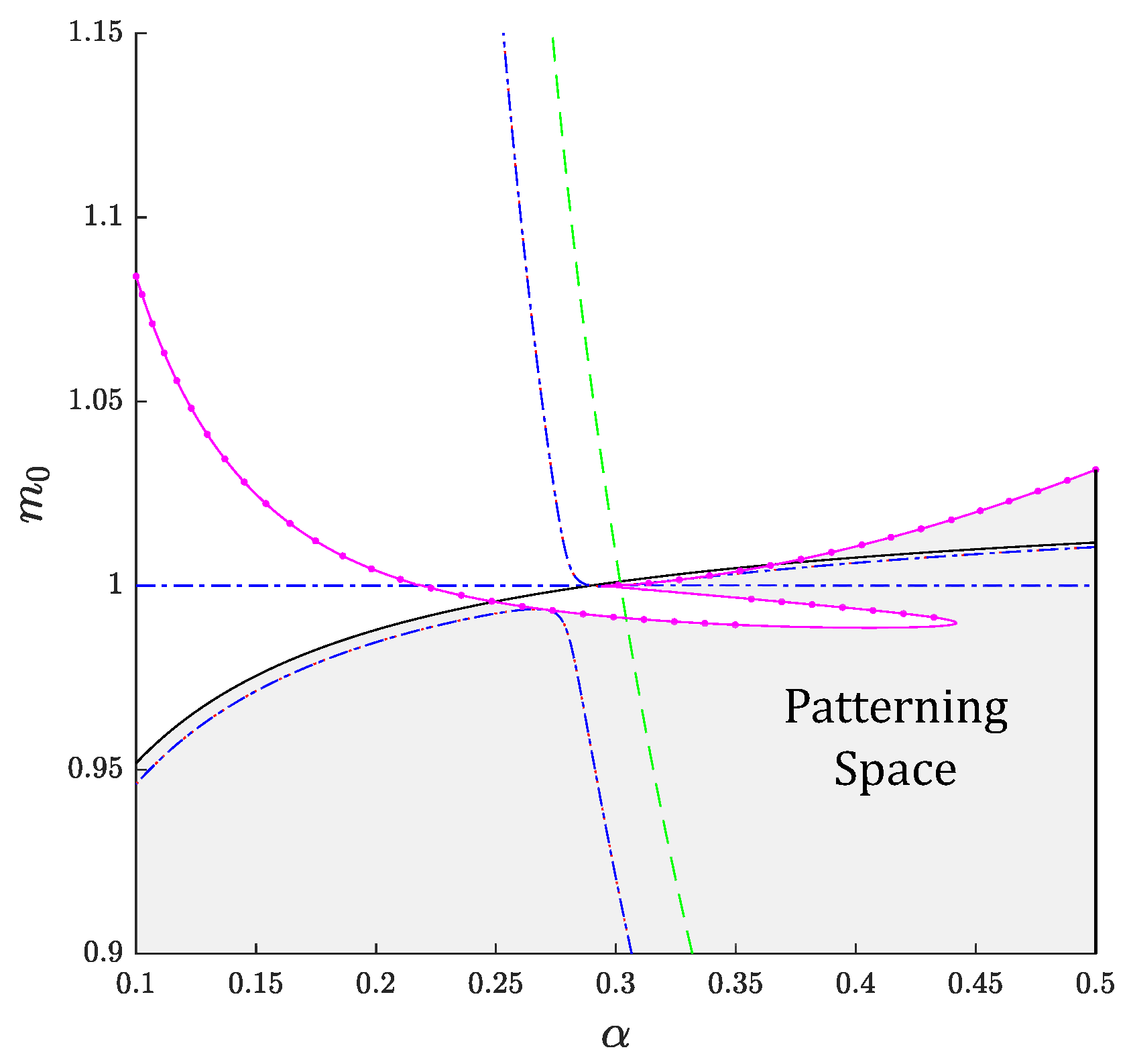
Condition (15b) highlights the effect of poromechanics towards the instability of the system, in comparison against the uncoupled cased. Increasing the influence of the mesenchymal cells through τ , or the influence of mechanics on f through ξ f , can relax the requirement that the feedback-positive loop from (14b) should be sufficiently strong to create instability. As mentioned in the activation/inactivation of epithelium scenario, this will depend mostly on the sign of the active stress component of the coefficient, and thus on the sign of τ and the value of m 0 , see Figure 2(C1). The dispersion relation for the ( m 0 , α ) - and ( κ 1 , κ 2 ) – parameter spaces illustrates how, for the same fixed set of parameters from Box 1, the poromechanical coupling leads to a decrease of the critical parameter value (Figure 2(A3,B3)). Unfortunately, the ease to push the system to instability is counter-balanced by a more restrictive space of parameters values where patterns can be formed (more precisely, compared to Figure 1(A1,B1) and Figure 2(A1,B1,C1)). This can increase the difficulty in tuning parameters to produce specific patterns. Indeed, zooming into the parameter pair ( m 0 , α ) on the region where the boundary conditions cross (see Figure 3), exposes how easily the patterns can disappear after a relatively small variation in parameter values.

4. Extension to Finite-Strain Poroelasticity and Growth

We briefly recall some kinematic considerations, needed in order to incorporate growth effects. Thorough reviews of mechanical models for growth of soft living tissues can be found in [17,18]. Let us denote by X the position of a material point in the reference (or initial) configuration (region Ω 0 with boundary Ω 0 = Γ 0 Σ 0 and outward pointing unit normal N 0 ) and let x = φ ( X ) denote its position at time t in the current configuration of the domain, Ω , determined by the deformation mapping φ ( · , t ) : Ω 0 Ω . We adopt the notation Div , Div for the divergence of tensor and vector fields, and Grad , Grad for the gradients of vector and scalar fields, respectively; all with respect to the material coordinates. The geometric deformation tensor is F = Grad φ = I + Grad u and its Jacobian is J = det F > 0 . The velocity in Lagrangian coordinates is denoted as v = u ˙ , and  C = F F is the right Cauchy–Green strain tensor.
As in the linearised regime, we assume that the region occupied by the tissue is fully saturated, and consisting of a fluid and of a solid phase:
ϕ f + ϕ s = 1 ,
where the ϕ j ’s denote the volume fraction of each phase. The phase s is assumed a neo–Hookean solid whereas the liquid phase is considered as an ideal fluid. Both phases are assumed intrinsically incompressible. The expected growth is due to proliferation of cells, and implying a mass exchange between the phases. The mass balances in the Eulerian framework assume the form
ϕ s t + div ( ϕ s v s ) = r s in Ω × ( 0 , t final ] ,
ϕ f t + div ( ϕ f v f ) = r s in Ω × ( 0 , t final ] ,
with v s , v f the Eulerian velocities in each phase, and  r s = α 0 ϕ s ( 1 ϕ s ) ( m m 0 ) being the mass growth rate (net proliferation rate of cells in the solid phase), here assumed linearly dependent on the concentration of mesynchemal cells and decreasing as the available space decreases. In turn, the general form of the momentum balances is
div ( ϕ s σ eff , s ) ϕ s p + f s f = 0 in Ω × ( 0 , t final ] , div ( ϕ f σ eff , f ) ϕ f p + f f s = 0 in Ω × ( 0 , t final ] ,
where the σ eff , j ’s are the respective effective Cauchy stresses, p is the average pressure of the liquid phase, and 
f s f = p ϕ s + η / κ ϕ s ϕ f ( v f v s ) , f f s = p ϕ f η / κ ϕ f ϕ s ( v f v s ) ,
denote drag terms and net sources of momentum, where κ , η are the permeability and dynamic viscosity, respectively. The effective stress of the liquid phase σ eff , f is assumed negligible with respect to the interstitial pressure gradient and therefore the mixture stress is σ eff = σ eff , s . In addition, Darcy’s law gives
v f v s = κ η ϕ f p ,
and then the mixture momentum balance is written as
div ( σ eff ) + p = 0 in Ω × ( 0 , t final ] .
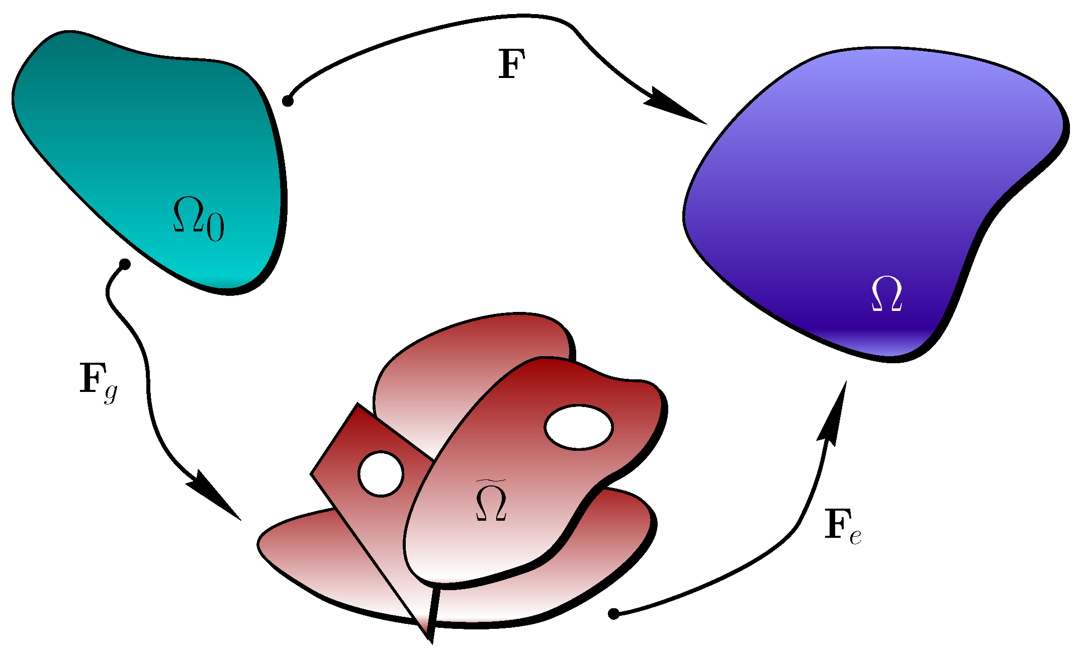
The deformation mapping can be decomposed into a purely growth part and the remainder, elastic, deformation. Such splitting implies that there exists an intermediate configuration Ω ˜ between Ω 0 and Ω which is not necessarily compatible (and which we assume is completely stress free, see sketch in Figure 4), and consequently a multiplicative decomposition of the deformation gradient into a growth deformation gradient (describing local generation or removal of material points) and an elastic deformation gradient tensor is admitted (see, for instance, [35,36,37]).
F = F e F g ,
and therefore J = J e J g with J e : = det F e , J g : = det F g . Note also that since F is assumed nonsingular, so are the tensors F e , F g .
Since the intermediate configuration is considered stress-free, stresses are exerted only by the elastic deformation, and the constitutive relations between a given strain energy function Ψ (that characterises the material response of the solid for hyperelastic materials) and the measures of stress can be stated with respect to the intermediate configuration Ω ˜ . For the Cauchy stress this gives
σ eff = 2 J e 1 F e Ψ C e F e ,
where C e = F e F e and J e = det ( F F g 1 ) is the reversible part of the Jacobian. This constitutive equation requires to describe also F and F g , but from the relation F ˙ F 1 = v s , we realise that only F g needs to be specified.
In order to translate Equations (18a)–(22) into Lagrangian form, we recall the change in volume and area relations d V = J d V 0 and d S = J F d S 0 together with the transformation of unit outward normal vectors = F N 0 . For the solid mass balance (18a) it suffices to apply Reynolds transport theorem, the change of coordinates, and Maxwell’s localisation to obtain
J ϕ s ¯ ˙ = J r s .
The Lagrangian form of Darcy’s law
v f v s = F κ η ϕ f C 1 Grad p ,
results from (19) in combination with transport, localisation, as well as pull-back operations. For the liquid mass balance (18b), one can apply the generalised Reynolds transport theorem (24), divergence’s theorem, and localisation, to arrive at
J ϕ f ¯ ˙ + Div ( J κ η C 1 Grad p ) = J r s .
Summing up (23) and (25) and taking an approximation of the fluid volume fraction in terms of fluid pressure and volume change we obtain (28b), below.
For transforming the momentum balance (20) we use the divergence theorem, the change of coordinates, we recall the relation between Cauchy and first Piola–Kirchhoff stress P = J σ F , and use again the divergence theorem to get (28a), below. The hyperelastic component to the stress is
P e = Ψ F | Ω ˜ ,
and for a neo–Hookean material, Equations (21)–(26) imply that the effective stress tensor is
P e = J ( μ B e ψ I ) F ,
where μ is the shear modulus, ψ denotes a Lagrange multiplier, and B e = F e F e is the right Cauchy–Green deformation tensor associated with the intermediate configuration Ω ˜ . Note that in this context, rather than material incompressibility of the mixture, the Lagrange multiplier ψ enforces a mass conservation kinematic constraint of the form J e = 1 , confirming that for a hyperelastically incompressible material all volume changes are solely due to growth factors ( J g = det F g is in turn irreversible) [38]. If  J g > 1 the body undergoes growth.
In summary, the equations of nonlinear poroelasticity with growth (including momentum conservation of the solid-fluid mixture, fluid mass balance, and incompressibility of elastic deformations) read as follows
ρ u ¨ Div ( P e + P f ) = 0 in Ω 0 × ( 0 , t final ] ,
C 0 p + α B W [ tr C d ] ¯ ˙ 1 J Div κ η J C 1 Grad p = in Ω 0 × ( 0 , t final ] ,
J e = 1 in Ω 0 × ( 0 , t final ] ,
where the stress exerted by the fluid (when pulled back to the reference configuration) is simply P f = α B W J p F , and the divergence and gradient operators are now understood with respect to the undeformed coordinates. In contrast with the model from Section 2, now the fluid has a source that we relate to the growth process and make it precise below. The divergence of displacement accompanying the Biot–Willis constant has now been replaced by tr C d , where d is the spatial dimension. The first term on the left-hand side of (28b) represents the rate of change of the total amount of fluid.
It remains to characterise the growth deformation gradient. We suppose that growth occurs due to a set of internal variables γ 1 , γ 2 , γ 3 acting on local orthonormal directions k 1 , k 2 , k 3 in the undeformed configuration (and in 2D we consider only γ 1 , γ 2 acting on k 1 , k 2 , respectively), and a general form for the growth deformation tensor is simply
F g = I + γ 1 k 1 k 1 + γ 2 k 2 k 2 + γ 3 k 3 k 3 .
Assuming that a transversely isotropic growth due to a constant rate occurs on the plane ( k 1 , k 2 ) and the growth due to morphogen concentrations acts mainly on the direction k 3 , we employ the following specification for the growth factors γ i :
γ 1 = δ 1 t , γ 2 = δ 1 t , γ 3 = δ 2 t + δ 3 m 1 + m 2 ,
where δ 1 , δ 2 , δ 3 are positive constants and we recall that m is the concentration of mesenchymal cells in the form used in the active stress from (5). In the 2D case, (29) will be replaced by
γ 1 = γ 2 = δ 2 t + δ 3 m 1 + m 2 .
As in [19,39] a more general description that defines a functional relation between the rates of the growth factors and the exchange of mass implies a dependence on the solid volume fraction
i = 1 d γ i ˙ γ i = r s ϕ s .
Following [30], we can write a constitutive equation for the mass source in (28b) depending on the constants γ i as follows
= 0 ( 2 δ 1 + δ 2 + δ 3 m ( γ 3 ) t m ) ,
where 0 is a constant and where we stress that ρ in this section refers to the density of the solid in the reference configuration.
The set of equations is complemented with suitable boundary and initial conditions, formulated in the reference configuration. In contrast with (7b)–(7c), here we impose Robin conditions for the poroelasticity on the whole undeformed boundary
( P e + P f ) N 0 + ξ R J F u = 0 on ( Γ 0 Σ 0 ) × ( 0 , t final ] ,
κ η J C 1 Grad p · N 0 = 0 on Γ 0 × ( 0 , t final ] , p = p D on Σ 0 × ( 0 , t final ] ,
where ξ R is the stiffness of the springs attached to Ω 0 .
Moreover, the chemotaxis system is recast in the reference domain. In particular, the advection terms are absorbed by the material derivatives (since we are assuming that all species are transported by the whole mixture and can diffuse in both phases) and the diffusion coefficients are modified by the Piola transformation. As in (28b), the divergence of displacement in the sink term from (3c) now is replaced by tr C d . The transformation also involves Reynolds transport theorem, divergence theorem, and localisation. Assuming that D m , D f , D b are isotropic, we have
m ˙ 1 J Div D m J C 1 Grad m α m exp ( γ m ) J C 1 Grad f = 0 in Ω 0 × ( 0 , t final ] ,
e ˙ [ κ 1 w ( X , t ) h 1 ( m ) + κ 2 h 2 ( m ) ] ( 1 e ) + [ 1 h 1 ( m ) ] ( κ 3 + κ 4 b ) e = 0 in Ω 0 × ( 0 , t final ] ,
f ˙ 1 J Div D f J C 1 Grad f κ F e + δ F f + ξ f ( tr C d ) = 0 in Ω 0 × ( 0 , t final ] ,
b ˙ 1 J Div D b J C 1 Grad b κ B h 3 ( m ) m + δ B b = 0 in Ω 0 × ( 0 , t final ] ,
where divergence and gradients are taken with respect to the undeformed configuration, and the zero-flux boundary conditions (7a) are changed accordingly
D m J C 1 Grad m α m exp ( γ m ) J C 1 Grad f · N 0 = D f J C 1 Grad f · N 0 = D m J C 1 Grad m · N 0 = 0 on Ω 0 × ( 0 , t final ] .

5. Numerical Tests

5.1. Discretisation and Implementation

We have employed mixed finite element methods for the spatial discretisation of systems (3a)–(5) and (28a)–(33d). We use quasi-uniform triangular/tetrahedral meshes in all cases. For the first system described in Section 2, since the linear poroelasticity equations are away from the nearly incompressibility limit (here the Poisson ratio is ν = 0.4 ), it suffices with using piecewise linear and continuous approximation of solid displacements (as well for all other unknowns). For the system proposed in Section 4, we employ the so-called Taylor–Hood mixed approximation of solid displacements and solid pressure composed by piecewise quadratic and continuous functions for each displacement component combined with piecewise linear and overall continuous functions for the solid pressure (this pair is known to satisfy an adequate inf-sup condition for the linearised hyperelasticity equations, see, e.g., [40]); and the fluid pressure as well as the chemical species concentrations are approximated with piecewise linear and continuous polynomials. For all problems, an outer fixed-point algorithm decouples the chemotaxis system from the poromechanics. An implicit-explicit method is employed to generate a full discretisation of the chemotaxis system and of the linear poroelasticity equations from Section 2, whereas for the poroelastic-growth system (28a)–(28c) with boundary conditions (32a)–(32b), an inner Newton–Raphson method is used to solve the corresponding nonlinear equations written in implicit form. All routines for the 2D tests have been implemented in the open-source finite element library FEniCS [41]. The solution of all nonlinear systems was carried out with Newton’s method using a tolerance of 10 7 .on either the relative or absolute 2 norm of the vector residuals, and the linear systems on each step were solved with the distributed direct solver MUMPS. For the 3D case we used the Firedrake library [42] (mainly due to its facility in handling block preconditioners). We provide details regarding the preconditioners in Section 5.3. The nonlinear tolerances are taken identical to the 2D case. For the linear solvers, we use a GMRES with the nested Schur preconditioner recently proposed in [8], with an absolute tolerance of 10 12 and a relative one of 10 2 . The use of such a big relative tolerance yields a simplified inexact-Newton method [43] that results in more nonlinear iterations requiring much less time.

5.2. Mesh Independence Study

To experimentally assess the convergence of the proposed finite element method, we employ two tests. One study confirms that the Galerkin discretisation, when using the finite element spaces specified above, provides optimal (first-order) convergence with respect to mesh refinement (measured in the H 1 -norm for all variables), where we simply use manufactured smooth solutions. The resulting convergence study is portrayed in Table 1, where r denotes the experimental convergence rates computed as
r = log ( err / err ^ ) [ log ( h / h ^ ) ] 1 ,
where err and err ^ denote errors produced on two consecutive meshes associated with mesh sizes h and h ^ , respectively.
The second study determines the mesh resolution we employ to conduct the numerical simulations of growth in the linear and nonlinear regimes. For this we only run a test on the linear regime up to t = 100 and simulating a single propagating wave. As an indicator we use a relative error (measured as the relative 2 norm of the residual) with respect to a fine-mesh computation where the reference solution is computed on a mesh of approximately 300 K elements. The coarsest mesh I has 30 K elements and in the three cases we have used a graded mesh (locally refined near the edge x = 0 , where we expect the primation to initiate). The outcome of the mesh independence test is displayed in Table 2, from which we select mesh II for the subsequent 2D tests, since the relative error produced with this mesh is sufficiently small.
We also note that while the method does converge for much coarser meshes, grids as fine as meshes I, II, III are required to capture small features (for example, the spatial random distributions in the initial perturbations used, for example, in Section 5.4 below).

5.3. Efficient Preconditioners

Given that we are using a Newton solver, an efficient preconditioner is fundamental to obtain computational times that are feasible for the 3D case. The splitting strategy we are considering allows us to consider the poroelastic and chemotaxis problems separately, where each of them considers a different preconditioning strategy. In what follows we give the details of the preconditioners used for the solution of the tangent operator for each physics.
  • Chemotaxis. This problem considers four similar building block physics, consisting essentially of three parabolic problems ( m , f , b ) and one algebraic constraint ( e ) . We consider an additive block solver, meaning that we use a block-wise Jacobi preconditioner with only the diagonal block of each variable. At the block level, we consider the action of an AMG preconditioner for the parabolic problems and the action of a Jacobi preconditioner for the algebraic one.
  • Poromechanics. The poromechanics block is more difficult, which is reflected in the complexity of the preconditioner under consideration. It is based on the block preconditioner proposed in [8] for large-strain poromechanics, where we use a lower Schur complement block factorisation with the fields u and ( ψ , p ) . For such a block we consider the action of an AMG preconditioner, whereas for the corresponding Schur complement block we consider instead a sparse representation given by an ad hoc extension of the fixed-stress splitting scheme proposed in [25]. For this, we add two stabilisation terms given by
    Ω 0 β s ψ ψ * + β f p p * d x ,
    where we have denoted with ( · ) * the test function corresponding to each variable and have used the values β s = β f = 0.1 . As this approach yields a sparse operator that approximates the Schur complement, we simply use the action of an AMG preconditioner based on it.
We highlight that the proposed preconditioner represents an improvement over [8], as we employ only preconditioner actions on each block, which allows us to use a GMRES linear solver instead of a flexible GMRES (which can be substantially more demanding in terms of computational cost). To assess the performance of the preconditioner, we consider only the first time instant of simulation, and report the nonlinear iterations, the maximum GMRES iterations per nonlinear iteration and the CPU times in Table 3.

5.4. Suppressed Solid Motion vs. Periodic Boundary Traction

In order to emphasise the effect of the stretch and deformation on the formation of patterns we compare the concentration of mesenchymal cells in two cases, one where the motion of the domain is suppressed (by setting τ = 0 ), and another scenario where the bottom of the domain, ( Γ ) , is kept clamped, the top of the domain undergoes a (relatively small) periodic traction, and the vertical faces are kept with zero traction. In this case we employ the linear poroelastic model from Section 2, and a zero fluid pressure flux is imposed on Σ = Ω \ Γ . The spatial domain is a square Ω = ( 0 , 20 ) 2 discretised into 58,482 triangular elements, and the model parameters that are modified with respect to those in Box 1 adopt the values
m 0 = 0.75 , D m = 0.03 , τ = ξ f = 0.001 .
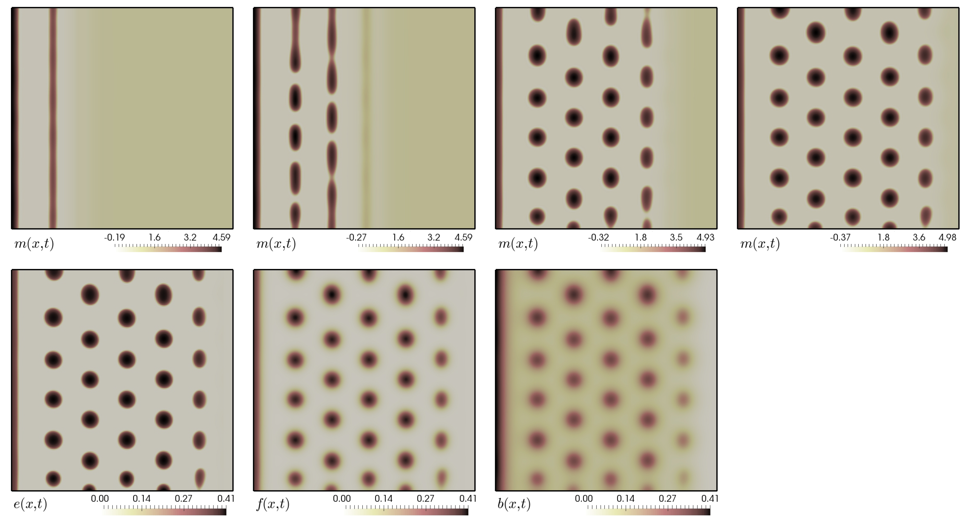
The initial conditions correspond to uniformly distributed random perturbations of 10% with respect to the steady state m 0 , e 0 , b 0 and of 1% with respect to the steady state f 0 . The traction is t = ( 0 , s 0 sin ( π t / t ^ ) ) , with magnitude s 0 = 1500 and period t ^ = 320 . We employ a fixed time step Δ t = 0.2 and advance the system until t = 520 . The outcome of these tests is collected in Figure 5 and Figure 6, where we observed that slight modifications in the poromechanics result in quite drastic alterations of the clustering of mesenchymal cells. For instance, in Figure 6 we see that on the bottom edge of the domain (where displacements are zero during the whole simulation), the relatively large stretches applied elsewhere on the body do not break the formation of dotted-shaped patterns at early stages, but they are swept away as time advances.

5.5. Finite Growth in 2D

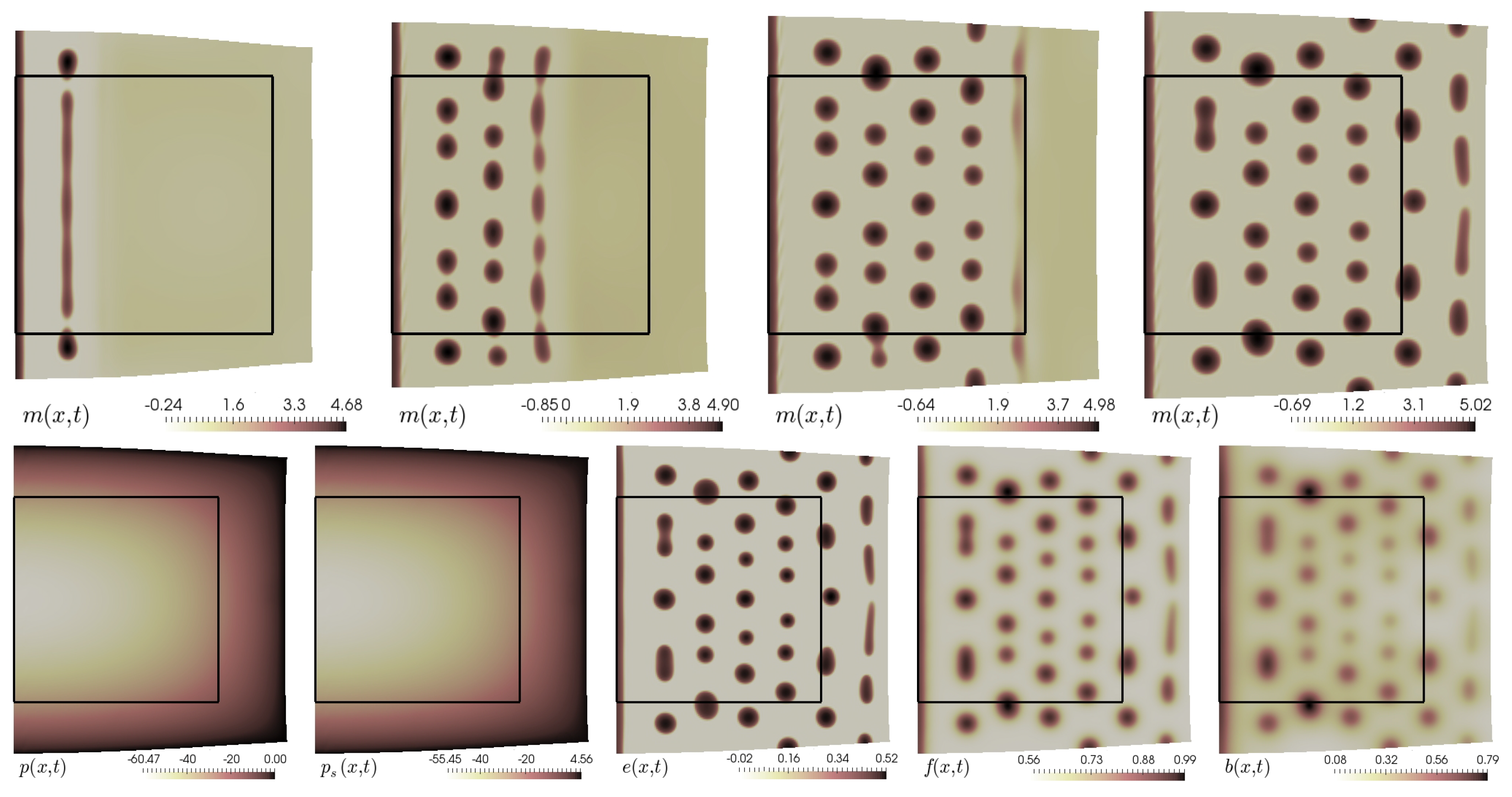
Next we maintain the domain and most model parameters as in the previous case and focus on the coupled model defined in Section 4. Determining the total first Piola–Kirchhoff stress from (27) and the growth specification (30) (with δ 2 = 0.15 , δ 3 = 0.045 ), we modify also the boundary treatment and consider that Γ 0 is the left edge of the domain whereas the remainder of Ω 0 is Σ 0 . On Γ 0 we impose zero normal displacement u · N 0 = 0 and a Robin boundary condition with constant ξ R = 0.0001 is set on Σ 0 . The shear modulus is μ = 4 , the solid permeability is augmented to κ = 0.001 , and we take ξ f = 0.3 . The fluid mass source is specified by (31) with 0 = 0.001 .
The panels in Figure 7 display transients of the growth of the initial domain and we plot the concentration of mesenchymal cells on the deformed configuration. We can observe that the patterns follow a different alignment than those formed in Figure 5, in particular disrupting the symmetry and the size distribution of the dotted-shaped patterns. The plots in the bottom row show the fluid and solid pressure together with the remaining chemical concentrations at the final time. Note that both solid and fluid pressures accumulate near Σ 0 . In addition, we note that the values of FGF at later times are negative since the last term on the left-hand side of (33c) represents a sink of f as the domain only grows (and tr C d is non-negative) throughout the simulation. We then change the sign of ξ f = 0.3 and obtain positive FGF concentrations as well as similar patterns in all fields (but exhibiting a higher wave-number than in the previous case). The results from these tests are shown in Figure 8, which confirm a qualitative agreement with numerical tests from [6] and also with the actual patterns observed in nature.

5.6. Finite Growth in 3D

To close this section we proceed to extend the previous example to the 3D case. The undeformed domain is still a simple geometry Ω 0 = ( 0 , 20 ) × ( 0 , 20 ) × ( 0 , 1 ) , where to obtain an accurate solution we used 140 elements per side in the X 1 and X 2 directions, and instead considered only 8 in the X 3 direction. This results in roughly 10 million degrees of freedom. The sides at X 1 = 0 and X 3 = 0 constitute Γ 0 , where zero normal displacements are considered, and on the remainder of the boundary we set Robin conditions as above, but using ξ R = 0.001 . The growth factors are considered as in (29) with the specification δ 1 = 1 / 52 , δ 2 = 0 , δ 3 = 1 / 104 . The results are shown in Figure 9, where we plot the evolution of the chemicals in the deformed configuration, and where the outline of the undeformed domain is also shown for visualisation purposes. We can see that as time progresses, the transversally isotropic growth depending only on time occurs mainly in the plane X 1 X 2 as in the 2D case. Most interestingly, the mesenchymal concentration exhibits new complex structures. From the upper view, an arrow-like structure can be seen, where from higher concentrations appear more distant when going from right to left. From the slice view below, it can be seen how these distant concentrations are instead connected within the geometry. We stress that this type of patterns can only be described by the 3D model and currently there are no available results in the literature of mathematical and numerical methods to guide a qualitative/quantitative comparison. We also emphasise that the observed patterns are not necessarily representative of the actual primordial patterns—which are mainly composed by independent buds—and therefore this aspect still requires further investigation.

6. Concluding Remarks

We have proposed a model for describing the interaction between poroelastic deformations and chemotactical displacement of mesenchymal cells, FGF, BMP and epithelium. This new model is based on the theoretical framework developed in [6] for a rigid domain. In our first family of models, the coupling mechanisms include degradation of FGF due to local solid compression, advection of chemicals through solid velocity, and an active stress driven by mesenchymal cells. We have derived a set of conditions for Turing patterns to emerge, focusing on the two-way coupling and the main coupling variables. The analytical results on the stability of the steady solutions are confirmed by numerical solutions that concentrate on the regime of infinitesimal strains. Our numerical simulations reveal that the homogeneous oscillations predicted by the linear stability analysis are destabilised for sufficiently large values of the coupling parameters. We have also investigated an extended model that accounts for growth and hyperelastic deformations of the solid matrix, and the coupling mechanisms in this case consist in intrinsic growth functions depending on time and on the concentration of mesenchymal cells, as well as modification of the diffusion coefficients in the chemotaxis model due to changes from spatial to reference coordinates.
The linear stability analysis for the nonlinearly coupled system from Section 4 could be carried out extending our results from Section 3 following the ideas from [38]. As the main application is on skin patterning for feather development, we could also incorporate growth models specifically targeted for shells or thin plates as in [44], and concentrate on bi-layered structures extending the formulations in [45]. Viscous effects might be required in the rheological assumptions leading to the construction of stress, where relevant works in that context include [46,47]. Another interesting direction of development concerns performing further testing and optimisation of robust preconditioners that are required for the more computationally demanding 3D simulations. Finally, we mention that we are currently working on developing the well-posedness analysis of the fully nonlinear coupling of poroelasticity and chemotaxis models.

Author Contributions

Conceptualization, M.C.M. and R.R.-B.; Formal analysis, L.M.D.O.V.; Investigation, N.A.B., L.M.D.O.V. and R.R.-B.; Methodology, N.A.B., L.M.D.O.V. and R.R.-B.; Supervision, M.C.M.; Visualization, N.A.B., L.M.D.O.V. and R.R.-B.; Writing—original draft, L.M.D.O.V. and R.R.-B.; Writing—review & editing, N.A.B. and M.C.M. All authors have read and agreed to the published version of the manuscript.

Funding

This research was funded by Georges & Antoine CLARAZ foundation; the Swiss National Science Foundation (FNSNF, grants 31003A and CR32I3); the International Human Frontier Science Program Organisation (HFSP RGP0019/2017); the European Research Council (ERC, Advanced grant EVOMORPHYS) under the European Union’s Horizon 2020 research and innovation programme; the Monash Mathematics Research Fund S05802-3951284; and by the Australian Research Council through the Discovery Project grant DP220103160 and through the Future Fellowship grant FT220100496.

Conflicts of Interest

The authors declare no conflict of interest.

Appendix A. Proof of Proposition 1

The spatial derivatives in the scalar case follow trivially from the definition of f. Both scalar and vector time derivatives also follow directly from the definition of f , v . For the spatial derivatives of v , using the definition of the differential operators and denoting { e ^ n } 1 , , d , the standard basis vectors in R d , we can readily write
div v = n x n v n , 0 e i k · x + ϕ t = n i k n v n , 0 e i k · x + ϕ t = n i k n v n = i v · k , v = m x m v e ^ m = n , m x m v n , 0 e i k · x + ϕ t e ^ n e ^ m = n , m i k m v n , 0 e i k · x + ϕ t e ^ n e ^ m = n , m i k m v n e ^ n e ^ m = m i k m v e ^ m = i v k .
On the other hand, using (9a) we can then straightforwardly derive (9b) as follows
div ε ( v ) = div n , m i v n k m + v m k n 2 e ^ n e ^ m = n , m i 2 v n k n k m + v m k n 2 2 e ^ m = 1 2 m ( v · k ) k m e ^ m + k 2 v m e ^ m = ( v · k ) k + k 2 v 2 , t ε ( v ) = 1 2 ( t v + t v ) = ϕ 2 ( v + v ) = ϕ ε ( v ) , div ( θ I ) = θ = ( i v · k ) = i n x n ( v · k ) e ^ n = i n , m k m x n v m e ^ n = i 2 n , m k m k n v m e ^ n = n k n ( v · k ) e ^ n = ( v · k ) k , t θ = div t v = ϕ div v = ϕ θ .

References

  1. Keller, E.F.; Segel, L.A. Initiation of slime mold aggregation viewed as an instability. J. Theor. Biol. 1970, 26, 399–415. [Google Scholar] [CrossRef]
  2. Yang, X.; Dormann, D.; Münsterberg, A.E.; Weijer, C.J. Cell movement patterns during gastrulation in the chick are controlled by positive and negative chemotaxis mediated by FGF4 and FGF8. Dev. Cell 2002, 3, 425–437. [Google Scholar] [CrossRef] [Green Version]
  3. Lin, C.M.; Jiang, T.X.; Baker, R.E.; Maini, P.K.; Widelitz, R.B.; Chuong, C.M. Spots and stripes: Pleomorphic patterning of stem cells via p-ERK-dependent cell chemotaxis shown by feather morphogenesis and mathematical simulation. Dev. Biol. 2009, 334, 369–382. [Google Scholar] [CrossRef] [PubMed] [Green Version]
  4. Mou, C.; Pitel, F.; Gourichon, D.; Vignoles, F.; Tzika, A.; Tato, P.; Yu, L.; Burt, D.W.; Bed’Hom, B.; Tixier-Boichard, M.; et al. Cryptic patterning of avian skin confers a developmental facility for loss of neck feathering. PLoS Biol. 2011, 9, e1001028. [Google Scholar] [CrossRef] [PubMed] [Green Version]
  5. Painter, K.J.; Hunt, G.S.; Wells, K.L.; Johansson, J.A.; Headon, D.J. Towards an integrated experimental–theoretical approach for assessing the mechanistic basis of hair and feather morphogenesis. Interface Focus 2012, 2, 433–450. [Google Scholar] [CrossRef]
  6. Painter, K.J.; Ho, W.; Headon, D.J. A chemotaxis model of feather primordia pattern formation during avian development. J. Theor. Biol. 2018, 437, 225–238. [Google Scholar] [CrossRef] [Green Version]
  7. Coussy, O. Poromechanics; John Wiley & Sons: Hoboken, NJ, USA, 2004. [Google Scholar]
  8. Barnafi, N.; Gómez-Vargas, B.; Lourenço, W.J.; Reis, R.F.; Rocha, B.M.; Lobosco, M.; Ruiz-Baier, R.; Santos, R.W.d. Finite element methods for large-strain poroelasticity/chemotaxis models simulating the formation of myocardial oedema. J. Sci. Comput. 2022, 92, e92. [Google Scholar] [CrossRef]
  9. Lourenço, W.d.J.; Reis, R.F.; Ruiz-Baier, R.; Rocha, B.M.; Santos, R.W.d.; Lobosco, M. A poroelastic approach for modelling myocardial oedema in acute myocarditis. Front. Physiol. 2022, 13, e888515. [Google Scholar] [CrossRef] [PubMed]
  10. Barnafi, N.; Gregorio, S.D.; Dedè, L.; Zunino, P.; Vergara, C.; Quarteroni, A. A multiscale poromechanics model integrating myocardial perfusion and systemic circulation. SIAM J. Appl. Math. 2021, 82, 1113–1660. [Google Scholar]
  11. Vuong, A.-T.; Yoshihara, L.; Wall, W.A. A general approach for modeling interacting flow through porous media under finite deformations. Comput. Methods Appl. Mech. Eng. 2015, 283, 1240–1259. [Google Scholar] [CrossRef]
  12. Berger, L.; Bordas, R.; Burrowes, K.; Grau, V.; Tavener, S.; Kay, D. A poroelastic model coupled to a fluid network with applications in lung modelling. Int. J. Numer. Methods Biomed. Eng. 2016, 32, e02731. [Google Scholar] [CrossRef] [PubMed]
  13. Vilaca, L.M.D.O.; Gómez-Vargas, B.; Kumar, S.; Ruiz-Baier, R.; Verma, N. Stability analysis for a new model of multi-species convection-diffusion-reaction in poroelastic tissue. Appl. Math. Model. 2020, 84, 425–446. [Google Scholar] [CrossRef]
  14. Moeendarbary, E.; Valon, L.; Fritzsche, M.; Harris, A.R.; Moulding, D.A.; Thrasher, A.J.; Stride, E.; Mahadevan, L.; Charras, G.T. The cytoplasm of living cells behaves as a poroelastic material. Nat. Mater. 2013, 12, e3517. [Google Scholar] [CrossRef] [PubMed] [Green Version]
  15. Collis, J.; Brown, D.L.; Hubbard, M.E.; O’Dea, R.D. Effective equations governing an active poroelastic medium. Proc. R. Soc. A 2017, 473, e20160755. [Google Scholar] [CrossRef] [PubMed] [Green Version]
  16. Penta, R.; Ambrosi, D.; Shipley, R.J. Effective governing equations for poroelastic growing media. Q. J. Mech. Appl. Math. 2014, 67, 69–91. [Google Scholar] [CrossRef] [Green Version]
  17. Jones, G.W.; Chapman, S.J. Modeling growth in biological materials. SIAM Rev. 2012, 54, 52–118. [Google Scholar] [CrossRef]
  18. Kuhl, E. Growing matter: A review of growth in living systems. J. Mech. Behav. Biomed. Mater. 2014, 29, 529–543. [Google Scholar] [CrossRef]
  19. Mascheroni, P.; Carfagna, M.; Grillo, A.; Boso, D.P.; Schrefler, B.A. An avascular tumor growth model based on porous media mechanics and evolving natural states. Math. Mech. Solids 2018, 23, 686–712. [Google Scholar] [CrossRef]
  20. Moreo, P.; Gaffney, E.A.; García-Aznar, J.M.; Doblaré, M. On the modelling of biological 795 patterns with mechanochemical models: Insights from analysis and computation. Bull. Math. Biol. 2010, 72, 400–431. [Google Scholar] [CrossRef]
  21. Murray, J.D.; Maini, P.K.; Tranquillo, R.T. Mechanochemical models for generating biological pattern and form in development. Phys. Rep. 1988, 171, 59–84. [Google Scholar] [CrossRef] [Green Version]
  22. Radszuweit, M.; Engel, H.; Bär, M. An active poroelastic model for mechanochemical patterns in protoplasmic droplets of physarum polycephalum. PLoS ONE 2014, 9, e99220. [Google Scholar] [CrossRef] [PubMed]
  23. Barnafi, N.; Zunino, P.; Dedè, L.; Quarteroni, A. Mathematical analysis and numerical approximation of a general linearized poro-hyperelastic model. Comput. Math. Appl. 2021, 91, 202–228. [Google Scholar] [CrossRef]
  24. Berger, L.; Bordas, R.; Kay, D.; Tavener, S. A stabilized finite element method for finite-strain three-field poroelasticity. Comput. Mech. 2017, 60, 51–68. [Google Scholar] [CrossRef] [PubMed] [Green Version]
  25. Borregales, M.; Radu, F.A.; Kumar, K.; Nordbotten, J.M. Robust iterative schemes for non-linear poromechanics. Computat. Geosci. 2018, 22, 1021–1038. [Google Scholar] [CrossRef] [Green Version]
  26. Costanzo, F.; Miller, S.T. An arbitrary Lagrangian-Eulerian finite element formulation for a poroelasticity problem stemming from mixture theory. Comput. Methods Appl. Mech. Eng. 2017, 323, 64–97. [Google Scholar] [CrossRef]
  27. Korsawe, J.; Starke, G.; Wang, W.; Kolditz, O. Finite element analysis of poro-elastic consolidation in porous media: Standard and mixed approaches. Comput. Methods Appl. Mech. Eng. 2006, 195, 1096–1115. [Google Scholar] [CrossRef]
  28. Verma, N.; Gómez-Vargas, B.; Vilaca, L.M.D.O.; Kumar, S.; Ruiz-Baier, R. Well-posedness and discrete analysis for advection-diffusion-reaction in poroelastic media. Appl. Anal. 2022, 101, 4914–4941. [Google Scholar] [CrossRef]
  29. Kadeethum, T.; Lee, S.; Ballarind, F.; Choo, J.; Nick, H.M. A locally conservative mixed finite element framework for coupled hydro-mechanical–chemical processes in heterogeneous porous media. Comput. Geosci. 2021, 152, e104774. [Google Scholar] [CrossRef]
  30. Armstrong, M.H.; Tepole, A.B.; Kuhl, E.; Simon, B.R.; Geest, J.P.V. A finite element model for mixed porohyperelasticity with transport, swelling, and growth. PLoS ONE 2016, 11, e0152806. [Google Scholar] [CrossRef] [Green Version]
  31. Jin, L.; Zoback, M.D. Fully dynamic spontaneous rupture due to quasi-static pore pressure and poroelastic effects: An implicit nonlinear computational model of fluid-induced seismic events. J. Geophys. Res. Solid Earth 2018, 123, 9430–9468. [Google Scholar] [CrossRef] [Green Version]
  32. Luo, P.; Rodrigo, C.; Gaspar, F.J.; Oosterlee, C.W. Multigrid method for nonlinear poroelasticity equations. Comput. Visual. Sci. 2015, 17, 255–265. [Google Scholar] [CrossRef]
  33. Showalter, R.E. Diffusion in poro-elastic media. J. Math. Anal. Appl. 2000, 251, 310–340. [Google Scholar] [CrossRef] [Green Version]
  34. Routh, E.J. A Treatise on the Stability of a Given State of Motion: Particularly Steady Motion; Macmillan and Company: London, UK, 1877. [Google Scholar]
  35. Lee, E.H. Elastic-plastic deformation at finite strains. J. Appl. Mech. 1969, 36, 1–6. [Google Scholar] [CrossRef]
  36. Rodriguez, E.K.; Hoger, A.; McCulloch, A.D. Stress-dependent finite growth in soft elastic tissues. J. Biomech. 1994, 27, 455–467. [Google Scholar] [CrossRef]
  37. Kida, N.; Morishita, Y. Continuum mechanical modeling of developing epithelial tissues with anisotropic surface growth. Finite Elem. Anal. Des. 2018, 144, 49–60. [Google Scholar] [CrossRef]
  38. Amar, M.B.; Goriely, A. Growth and instability in elastic tissues. J. Mech. Phys. Solids 2005, 53, 2284–2319. [Google Scholar] [CrossRef]
  39. Giverso, C.; Scianna, M.; Grillo, A. Growing avascular tumours as elastoplastic bodies by the theory of evolving natural configurations. Mech. Res. Commun. 2015, 68, 31–39. [Google Scholar] [CrossRef]
  40. Braess, D.; Ming, P. A finite element method for nearly incompressible elasticity problems. Math. Comp. 2005, 74, 25–52. [Google Scholar] [CrossRef] [Green Version]
  41. Alnæs, M.S.; Blechta, J.; Hake, J.; Johansson, A.; Kehlet, B.; Logg, A.; Richardson, C.; Ring, J.; Rognes, M.E.; Wells, G.N. The FEniCS project version 1.5. Arch. Numer. Softw. 2015, 3, 9–23. [Google Scholar]
  42. Rathgeber, F.; Ham, D.A.; Mitchell, L.; Lange, M.; Luporini, F.; McRae, A.T.T.; Bercea, G.T.; Markall, G.R.; Kelly, P.H.J. Firedrake: Automating the finite element method by composing abstractions. ACM T. Math. Softw. (TOMS) 2016, 43, 1–27. [Google Scholar] [CrossRef] [Green Version]
  43. Dembo, R.S.; Eisenstat, S.C.; Steihaug, T. Inexact Newton methods. SIAM J. Numer. Anal. 1982, 19, 400–408. [Google Scholar] [CrossRef]
  44. Dervaux, J.; Ciarletta, P.; Amar, M.B. Morphogenesis of thin hyperelastic plates: A constitutive theory of biological growth in the Föppl–von Kármaán limit. J. Mech. Phys. Solids 2009, 57, 458–471. [Google Scholar] [CrossRef]
  45. Vilaca, L.M.D.O.; Milinkovitch, M.C.; Ruiz-Baier, R. Numerical approximation of a 3D mechanochemical interface model for skin patterning. J. Comput. Phys. 2019, 384, 283–404. [Google Scholar]
  46. Bociu, L.; Guidoboni, G.; Sacco, R.; Webster, J.T. Analysis of nonlinear poro-elastic and poro-visco-elastic models. Arch. Ration. Mech. Anal. 2016, 222, 1445–1519. [Google Scholar] [CrossRef] [Green Version]
  47. Kaouri, K.; Méndez, P.E.; Ruiz-Baier, R. Mechanochemical models for calcium waves in embryonic epithelia. Vietnam J. Math. 2022, 50, 947–975. [Google Scholar] [CrossRef]
Figure 1. Patterning space, parameter condition and dispersion relations for the uncoupled poro–mechano–chemical model. (A1) Predicted patterning space for a selected interval in ( m 0 , α ) parameter space: (green plain) boundary constructed from (14a); (red-dashed) boundary coming from (14b); (blue–dot–dashed) boundary built from (14c). (A2) Parameter coefficient condition a0 Curves are drawn from the critical value m 0 c (green) and for 25% and 50% increase/decrease parameter values. (A3) Associated dispersion relations. Colour code is kept identical with (A2). (B1B3) Similar analysis for the ( κ 1 , κ 4 ) parameter space.
Mathematics 10 04096 g001
Figure 2. Patterning space, parameter condition and dispersion relations for the coupled poro–mechano–chemical model. (A1): predicted patterning space for a selected interval in ( m 0 , α ) . Parameter space: (black plain) boundary built from (15a) for θ 1 ; (green-dashed) boundary built from (15a) for θ 2 ; (red-dot-dot) boundary built from (15b); (blue–dot–dashed) boundary from (15c); (magenta-dot-plain) boundary built from (16). (A2): Coefficient condition on d 0 . Curves are drawn from the critical value m 0 c (green) and for the 25% and 50% increase/decrease parameter value. (A3): associated dispersion relations. Colour code is kept identical with (A2). (B1B3): similar analysis for the ( κ 1 , κ 4 ) parameter space. (C1C3): similar analysis for the ( τ , ξ f ) parameter space.
Mathematics 10 04096 g002aMathematics 10 04096 g002b
Figure 3. Patterning space for the coupled poro-mechano-chemical model. Selected interval in the ( m 0 , α ) parameter space. (black plain) boundary built from (15a) for θ 1 ; (green-dashed) boundary from (15a) for θ 2 ; (red-dot-dot) boundary from (15b); (blue-dot-dashed) boundary from (15c); (magenta-dot-plain) boundary built from (16).
Mathematics 10 04096 g003
Figure 4. Decomposition of the tensor gradient of deformation F into pure growth F g and an elastic deformation tensor F e . The intermediate configuration Ω ˜ , between the undeformed reference state Ω 0 and the current/final configuration Ω including growth and elastic response with stress, is an incompatible and stress-free growth state.
Mathematics 10 04096 g004
Figure 5. Evolution of the mesenchymal cell concentration at t = 160 , 280 , 400 , 520 , under no deformation (top panels); and epithelium, FGF, and BMP concentrations at t = 520 (bottom).
Mathematics 10 04096 g005
Figure 6. Evolution of the mesenchymal cell concentration at t = 160 , 280 , 400 , 520 under periodic traction applied on the top edge of the domain (top); and snapshots of fluid pressure, epithelium, FGF, and BMP at t = 520 (bottom row).
Mathematics 10 04096 g006
Figure 7. Evolution of the mesenchymal cell concentration under finite growth using the formulation (30), snapshots are taken at t = 160 , 280 , 400 , 520 (first row). Bottom: plots at t = 520 of fluid pressure, solid pressure, epithelium, FGF, and BMP. Mechano-chemical coupling governed by ξ f = 0.5 .
Mathematics 10 04096 g007
Figure 8. Evolution of the mesenchymal cell concentration under finite growth using the formulation (30), snapshots are taken at t = 160 , 280 , 400 , 520 (top). Second row: plots at t = 520 of fluid pressure, solid pressure, epithelium, FGF, and BMP. Simulations using ξ f = 0.5 .
Mathematics 10 04096 g008
Figure 9. Evolution of the mesenchymal cell concentration under finite growth using the formulation (29), snapshots are taken at t = 160 , 280 , 400 , 520 (top). We also display the fluid and solid pressures (second row), the mesenchymal and epithelium concentrations (third row), and the FGF and BMP (fourth row).
Mathematics 10 04096 g009
Table 1. Accuracy verification test using continuous and piecewise linear elements for the approximation of all variables. Error history (number of degrees of freedom, errors in the H 1 -norm, and experimental convergence rates) with respect to smooth manufactured solutions computed at t = 10 . The symbol * indicates that the convergence rate is not computed for the coarsest level.
DoF u u h 1 r p p h 1 r m m h 1 r e e h 1 r f f h 1 r b b h 1 r
64 1.0 × 10 2 * 1.4 × 10 3 * 1.0 × 10 2 * 8.0 × 10 0 * 2.8 × 10 1 * 2.9 × 10 1 *
176 3.0 × 10 1 1.77 6.4 × 10 2 1.16 2.8 × 10 0 1.88 4.9 × 10 0 0.70 1.9 × 10 1 0.67 1.8 × 10 1 0.63
568 1.1 × 10 1 1.19 3.6 × 10 2 0.97 1.1 × 10 0 1.36 4.1 × 10 0 0.57 1.4 × 10 1 0.53 1.4 × 10 1 0.56
2024 5.0 × 10 0 1.08 1.7 × 10 2 1.19 5.1 × 10 1 1.09 3.3 × 10 0 0.61 8.5 × 10 0 0.73 8.6 × 10 0 0.73
7624 2.4 × 10 0 1.02 8.3 × 10 1 1.11 2.5 × 10 1 1.02 2.2 × 10 0 0.76 4.4 × 10 0 0.96 4.4 × 10 0 0.96
29,576 1.3 × 10 0 0.98 4.3 × 10 1 0.94 1.3 × 10 1 1.01 1.3 × 10 0 0.82 2.2 × 10 0 1.00 2.2 × 10 0 0.99
116,488 6.6 × 10 1 0.98 2.4 × 10 1 0.92 6.3 × 10 2 1.00 6.5 × 10 1 0.95 1.1 × 10 0 1.00 1.1 × 10 0 1.00
Table 2. Mesh independence test. Approximate number of triangular elements and of degrees of freedom, relative computational time, and relative error with respect to a fine mesh computation.
MeshCardinalityTotal DoFsCPU TimeError
I30 K110 K15%9%
II60 K218 K25%5%
III120 K430 K40%4%
Table 3. Performance of the nonlinear solver used with the preconditioner detailed in Section 5.3. We show the total CPU time on the nonlinear solver on a single timestep, together with the maximum number of GMRES iterations in parenthesis.
DoFs1 CPU2 CPUs4 CPUs8 CPUs12 CPUs16 CPUs
35280.57 (10)0.56 (10)0.68 (10)0.72 (10)0.77 (10)0.7 (10)
20,1721.01 (10)1.00 (9)1.01 (10)0.93 (10)1.25 (10)0.93 (10)
59,5362.35 (11)1.95 (9)1.46 (10)1.31 (9)1.03 (10)1.29 (10)
131,2205.43 (11)3.44 (10)2.48 (10)1.81 (10)1.63 (10)1.6 (10)
244,82410.72 (11)6.36 (11)4.35 (11)2.7 (10)2.59 (10)2.34 (10)
409,94819.03 (12)12.93 (12)7.09 (12)4.7 (12)3.72 (12)3.26 (12)
636,19231.57 (12)20.14 (12)11.27 (12)7.11 (12)5.38 (12)4.72 (12)
933,15649.81 (12)29.2 (12)16.24 (12)9.73 (12)7.55 (12)6.82 (12)
(a) Performance of chemotaxis solver.
DoFs1 CPU2 CPUs4 CPUs8 CPUs12 CPUs16 CPUs
16,8932.5 (8)1.8 (8)1.8 (8)2.05 (8)1.91 (8)2.17 (8)
108,50112.13 (12)7.27 (12)4.8 (12)3.11 (12)2.8 (12)2.89 (12)
337,22939.71 (13)22.62 (14)12.31 (14)7.57 (14)6.6 (14)5.72 (14)
765,47798.6 (14)52.06 (14)28.45 (14)16.5 (14)12.57 (14)10.79 (14)
1,455,645202.15 (14)102.76 (14)56.51 (14)32.32 (14)23.83 (14)19.58 (14)
2,470,133350.59 (14)192.52 (14)99.84 (14)55.04 (14)40.24 (14)33.75 (14)
3,871,341598.98 (15)324.14 (15)168.48 (15)89.02 (15)63.27 (15)54.29 (15)
5,721,669869.06 (15)462.3 (15)242.9 (15)130.09 (15)98.15 (15)78.02 (15)
(b) Performance of poromechanics solver.
Publisher’s Note: MDPI stays neutral with regard to jurisdictional claims in published maps and institutional affiliations.