Article

Data-Driven Constitutive Modeling via Conjugate Pairs and Response Functions

by
Victoria Salamatova
1,2,3
1
Marchuk Institute of Numerical Mathematics of the Russian Academy of Sciences, Moscow 119333, Russia
2
Scientific Center for Information Technology and Artificial Intelligence, Sirius University of Science and Technology, Sochi 354340, Russia
3
Institute for Computer Science and Mathematical Modeling, I. M. Sechenov First Moscow State Medical University (Sechenov University), Moscow 119991, Russia
Mathematics 2022, 10(23), 4447; https://doi.org/10.3390/math10234447
Submission received: 15 October 2022 / Revised: 11 November 2022 / Accepted: 23 November 2022 / Published: 25 November 2022
(This article belongs to the Special Issue Mathematical Modelling in Biomedicine III)

Abstract

:
Response functions completely define the constitutive equations for a hyperelastic material. A strain measure providing an orthogonal stress response, grants response functions directly from experimental curves. One of these strain measures is the Laplace stretch based on QR-decomposition of the deformation gradient. Such a recovery of response functions from experimental data fits the paradigm of data-driven modeling. The set of independent conjugate stress–strain base pairs were proposed as a simple alternative for constitutive modeling and thus might be efficient for data-driven modeling. In the present paper we explore applicability of the conjugate pairs approach for data-driven modeling. The analysis is based on representation of the conjugate pairs in terms of the response functions due to the Laplace stretch. Our analysis shows that one can not guarantee independence of these pairs except in the case of infinitesimal strain.

1. Introduction

Simulation of the mechanical behavior of soft tissues remains a challenge in many applications of biomechanics and biomedical engineering. Due to their complex structure, soft tissues demonstrate a nonlinear mechanical behavior [1]. Hyperelastic models are very popular in the mechanical description of soft tissues [2]. The standard approach to the mechanical model recovery is the following. First, one collects experimental data such as stress–strain curves under different loading conditions (e.g., tensile testing and/or shear testing). Second, one chooses a few hyperelastic models and fits them to existing experimental curves to find model parameters. Third, the best fitted hyperelastic model is used to describe the mechanical behavior under complex loading conditions.
The main problem of such an approach is the necessity to solve an ill-posed inverse problem, since the number of material model parameters is usually larger than the number of independent experimental data. This leads to the occurrence of multiple sets of optimal material model parameters for the same data sets [3]. Another issue of the standard approach is its predictive capability of the fitted hyperelastic model in case of limited experimental data [4]. The data-driven modeling seems to be a more appealing alternative approach to the recovery of constitutive equations from experimental data.
Response functions (partial derivatives of an elastic potential with respect to a strain measure) completely define the constitutive equation for a hyperelastic material [5,6]. A strain measure providing an orthogonal stress response, grants response functions directly from experimental curves [6,7]. One of these strain measures is the Laplace stretch based on QR-decomposition of the deformation gradient [8,9]. Such a recovery of response functions from experimental data fits the paradigm of data-driven modeling [10].
The seminal work of Freed et al. [11] suggests to use the Laplace stretch in order to construct a set of three independent conjugate stress/strain base pairs: “conjugate pairs ought to be chosen where paired responses are observed to be independent of one another”. Such a set of independent conjugate stress/strain pairs provides one-to-one mapping between conjugate pairs and solid stress-strain state. In other words, construction of constitutive equations for solids is assumed to be possible without any invariant-based theory. The authors highlight that independence of proposed conjugate pairs “cannot be proved theoretically, only disproved experimentally, if at all. If disproved for a certain scenario, that would not necessarily invalidate the utility of a particular conjugate pairing; rather, it would bracket its range of applicability”. The conjugate stress/strain base pairs approach has been actively extended to three-dimensional, anisotropic, and inelastic cases (see Refs. [12,13,14,15,16] and references within).
In the present paper we briefly review the above three approaches to the construction of the constitutive equation from experimental data, and explore the applicability of the conjugate pairs approach for data-driven modeling. The analysis is based on representation of the conjugate pairs in terms of the response functions due to the Laplace stretch. Two virtual experiments for a hyperelastic membrane (homogeneous planar deformation and circular membrane inflation) confirm the theoretical prediction.
The paper is organized as follows. In Section 2 we introduce basic notions for kinematics of the membrane. In Section 3 we review the above three approaches for data-driven deriving constitutive equations for isotropic hyperelastic materials. In Section 4 we present two virtual experiments for a hyperelastic membrane which confirm our theoretical analysis.

2. Kinematics

We consider a thin incompressible hyperelastic membrane whose deformation is described by the deformation of its mid-surface via the surface deformation gradient [17,18]
F 2 d = α = 1 2 g α G α .
Here g α are covariant basis vectors of an actual (deformed) mid-surface configuration, G α are contravariant basis vectors of a reference (undeformed) configuration, and operation ⊗ is the tensor product mapping vectors a , b to a matrix a b = a b T (for details, refer to Appendix A).
The assumption of a hyperelastic isotropic material model implies the existence of an elastic potential ψ = ψ ^ ( η i ) such that
σ = i ψ ^ η i A i ,
where σ is the Cauchy stress tensor, η i is a strain measure, ψ ^ / η i are response functions, A i are known tensors depending on η i . It is clear that constitutive equations σ = σ ( η i ) depend on the chosen strain measure. Strain measures η i satisfying A i : A j = tr ( A i A j T ) = δ i j grant explicit definition of the response functions:
ψ η i = σ : A i .
Here and after δ i j is the Kronecker delta.

3. Constitutive Equations

Below we review several approaches for the data-driven deriving constitutive equations for isotropic hyperelastic materials.

3.1. Constitutive Equation via Invariants of the Right Cauchy–Green Deformation Tensor

Various strain measures are based on the deformation gradient, the most popular measure is the right Cauchy–Green deformation tensor
C 2 d = F 2 d T F 2 d = α , β = 1 2 g α β G α G β , g α β = ( g α , g β ) .
For invariants of C 2 d
I 1 = tr C 2 d ,
I 2 = J 2 = det C 2 d .
the surface elastic potential has the form ψ = ψ ¯ ( I 1 , J ) and the main tension tensors (the second Piola–Kirchhoff tension tensor S 2 d , the Cauchy tension tensor σ 2 d , and the Kirchhoff tension tensor τ 2 d ) are as follows [17]:
S 2 d = S α β G α G β , S α β = 2 ψ ¯ I 1 G α β + J 2 ψ ¯ J g α β ; σ 2 d = 1 J F 2 d S 2 d F 2 d T = 2 J ψ ¯ I 1 G α β + J 2 ψ ¯ J g α β g α g β ;
τ 2 d = J σ 2 d = S α β g α g β .
Although the invariant-based approach has many advantages, one of its main drawbacks is “non-orthogonality”: the representation σ 2 d = i ( ψ ¯ / I i ) A i is based on non-orthogonal tensors A i : A j δ i j . This leads to errors amplification during the procedure of finding response functions [7]. Nevertheless, the invariant-based approach for data-driven constitutive modeling are appealing, see e.g., Refs. [19,20].

3.2. Constitutive Equation via Laplace Stretch

Laplace stretch is the strain measure based on the QR-decomposition of the deformation gradient [8,9]:
F 2 d = Q F ˜ 2 d , F ˜ 2 d = α , β = 1 2 F ˜ α β ϵ α ϵ β , [ F ˜ 2 d ] ϵ α ϵ β = F ˜ α β = F ˜ 11 F ˜ 12 0 F ˜ 22 .
Here Q = e β ϵ β is an orthogonal tensor, vector pairs e α , ϵ α are orthonormal: ( e α , e β ) = δ α β and ( ϵ α , ϵ β ) = δ α β . Construction of e β and ϵ β is discussed in Appendix B. Here and after, the subscript for matrix notation [ · ] ϵ α ϵ β indicates with respect to which base object ( ϵ α ϵ β ) entries of the matrix are computed.
Srinivasa [8] proposed to use the components of F ˜ 2 d as the new strain measure later referred to as the Laplace stretch [9]:
ξ 1 = ln F ˜ 11 , ξ 2 = ln F ˜ 22 , ξ 3 = F ˜ 12 / F ˜ 11 .
Since C 2 d is a symmetric positive definite tensor and
C 2 d = F 2 d T F 2 d = F ˜ 2 d T Q T Q F ˜ 2 d = F ˜ 2 d T F ˜ 2 d ,
one can find entries F ˜ α β via Cholesky factorization of matrix [ C 2 d ] ϵ α ϵ β = ( C α β ) [8]
F ˜ 11 = C 11 , F ˜ 12 = C 12 / F ˜ 11 , F ˜ 22 = C 22 F ˜ 12 2 .
The invariants (2) and (3) in terms of ξ i are
I 1 = F ˜ 11 2 + F ˜ 22 2 + F ˜ 12 2 = e 2 ξ 1 ( 1 + ξ 3 2 ) + e 2 ξ 2 ,
J = det F 2 d = det Q det F ˜ 2 d = F ˜ 11 F ˜ 22 = e ξ 1 + ξ 2 .
These expressions will be used in the next section.
Strain characteristics ξ 1 , ξ 2 , ξ 3 yielding an elastic potential ψ = ψ ˜ ( ξ 1 , ξ 2 , ξ 3 ) provide the “orthogonality” condition A i : A j = δ i j [8]:
σ 2 d = 1 J ψ ˜ ξ 1 e 1 e 1 + 1 J ψ ˜ ξ 2 e 2 e 2 + 1 J F ˜ 22 F ˜ 11 ψ ˜ ξ 3 e 1 e 2 + 1 J F ˜ 22 F ˜ 11 ψ ˜ ξ 3 e 2 e 1 ,
or in terms of the Kirchhoff tension tensor components:
τ 2 d = J σ 2 d = α , β = 1 2 τ ˜ α β e α e β τ ˜ 11 = ψ ˜ ξ 1 , τ ˜ 22 = ψ ˜ ξ 2 , τ ˜ 12 = F ˜ 22 F ˜ 11 ψ ˜ ξ 3 .
Equations (12) allow us to obtain tabulated data for response functions directly from experimental stress–strain curves. Examples of using strain measures ξ 1 , ξ 2 , ξ 3 for data-driven modeling are discussed in Ref. [10].

3.3. Constitutive Equation via Conjugate Stress/Strain Base Pairs

Freed et.al [11] propose to use the Laplace stretch for constructing conjugate stress/strain base pairs. The fundamental hypothesis for such pairs is orthogonality as well: “the governing tensors for stress and the rate of deformation can be encoded into a set of independent conjugate base pairs wherein each stress/strain conjugate pair is a scalar pair” [11]. This approach has been extended to three-dimensional and anisotropic cases [12,13,14,15].
For the simplest planar isotropic material (membrane) the conjugate stress/strain base pairs are:
π = τ ˜ 11 + τ ˜ 22 , δ = ln F ˜ 11 F ˜ 22 ,
σ = τ ˜ 11 τ ˜ 22 , ε = ln F ˜ 11 / F ˜ 22 ,
τ = F ˜ 11 F ˜ 22 τ ˜ 12 , γ = F ˜ 12 / F ˜ 11 .
It is claimed that “the dilation response { δ , π } , the squeeze response { ε , σ } , and the shear response { γ , τ } can all be varied separately and independently of one another (at least in principle)” [11]. The response functions (12) give us a tool to check this statement. To this end, we rewrite the conjugate pairs in terms of ξ i and the response functions ψ ˜ / ξ i :
π = τ ˜ 11 + τ ˜ 22 = ψ ˜ ξ 1 + ψ ˜ ξ 2 , δ = ξ 1 + ξ 2 2 ,
σ = τ ˜ 11 τ ˜ 22 = ψ ˜ ξ 1 ψ ˜ ξ 2 , ε = ξ 1 ξ 2 2 ,
τ = F ˜ 11 F ˜ 22 τ ˜ 12 = ψ ˜ ξ 3 , γ = ξ 3 .
According to the representation theorem for invariants for scalar value isotropic functions, any isotropic hyperelastic material can be represented by an elastic potential as a function of the principal invariants of the right Cauchy–Green deformation tensor [21]. In our two-dimensional case this implies the surface potential function ψ of two arguments I 1 , J , ψ = ψ ¯ ( I 1 , J ) . At the same time I 1 = I 1 ( ξ 1 , ξ 2 , ξ 3 ) and J = J ( ξ 1 , ξ 2 , ξ 3 ) are known functions (9) and (10). Since by the chain rule the response function are
ψ ˜ ξ 1 = ψ ¯ I 1 I 1 ξ 1 + ψ ¯ J J ξ 1 = 2 e 2 ξ 1 ( 1 + ξ 3 2 ) ψ ¯ , I 1 + e ξ 1 + ξ 2 ψ ¯ , J
ψ ˜ ξ 2 = ψ ¯ I 1 I 1 ξ 2 + ψ ¯ J J ξ 2 = 2 e 2 ξ 2 ψ ¯ , I 1 + e ξ 1 + ξ 2 ψ ¯ , J
ψ ˜ ξ 3 = ψ ¯ I 1 I 1 ξ 3 + ψ ¯ J J ξ 3 = 2 ξ 3 e 2 ξ 1 ψ ¯ , I 1 ,
where
ψ ¯ , I 1 : = ψ ¯ I 1 , ψ ¯ , J : = ψ ¯ J ,
we rewrite (16)–(18) in terms of δ , ε , γ :
π = ψ ˜ ξ 1 + ψ ˜ ξ 2 = 2 ( e 2 ξ 1 ( 1 + ξ 3 2 ) + e 2 ξ 2 ) ψ ¯ , I 1 + 2 e ξ 1 + ξ 2 ψ ¯ , J = = 2 ( e 2 δ e 2 ε γ 2 + 2 e 2 δ cosh 2 ε ) ψ ¯ , I 1 + 2 e 2 δ ψ ¯ , J ;
σ = ψ ˜ ξ 1 ψ ˜ ξ 2 = 2 ( e 2 ξ 1 ( 1 + ξ 3 2 ) e 2 ξ 2 ) ψ ¯ , I 1 = = 2 ( e 2 δ e 2 ε γ 2 + 2 e 2 δ sinh 2 ε ) ψ ¯ , I 1 ,
τ = ψ ˜ ξ 3 = 2 ξ 3 e 2 ξ 1 ψ , I 1 = 2 γ e 2 δ e 2 ε ψ ¯ , I 1 ,
where
cosh ε : = ( e ε + e ε ) / 2 , sinh ε : = ( e ε e ε ) / 2 .
Since ψ ¯ , I 1 = ψ ¯ , I 1 ( I 1 ( δ , ε , γ ) , J ( δ , ε , γ ) ) and ψ ¯ , J = ψ ¯ , J ( I 1 ( δ , ε , γ ) , J ( δ , ε , γ ) ) , formulas (22)–(24) show that the dilation response { δ , π } , the squeeze response { ε , σ } and the shear response { γ , τ } can not all be varied separately and independently: π = π ( δ , ε , γ ) , σ = σ ( δ , ε , γ ) , τ = τ ( δ , ε , γ ) .
In the next section, this general observation is illustrated by two virtual experiments representing real laboratory tests.

4. Independence of Conjugate Stress/Strain Base Pairs in Virtual Experiments

Let us check the orthogonality of the conjugate stress/strain base pairs for the simplest elastic potential of an incompressible neo-Hookean material. For neo-Hookean membrane with shear modulus μ and thickness H one has [18,22]:
ψ N H = μ H 2 ( I 1 + J 2 3 ) .

4.1. Homogeneous Deformation

We consider the simple homogeneous deformation of a membrane:
x 1 = a X 1 + a κ X 2 , x 2 = b X 2 .
In this case G α = G α = ϵ α = e α , α = 1 , 2 , and the surface deformation gradient is
[ F 2 d ] ϵ α ϵ β = a a κ 0 b .
In QR-decomposition the orthogonal tensor Q becomes the identity tensor I and F ˜ 2 d = F 2 d . The conjugate stress/strain pairs are
δ = ln a b , ε = ln a / b , γ = κ ,
and surface invariants are
I 1 = a 2 ( 1 + κ 2 ) + b 2 = e 2 δ e 2 ε γ 2 + 2 e 2 δ cosh 2 ε , J = a b = e 2 δ .
Therefore,
ψ , I 1 N H = μ H / 2 , ψ , J N H = μ H J 3 = μ H e 6 δ ,
and according to (22)–(24)
π = μ H e 2 δ ( e 2 ε γ 2 + 2 cosh 2 ε ) 2 μ H e 4 δ
σ = μ H e 2 δ ( e 2 ε γ 2 + 2 sinh 2 ε ) ,
τ = μ H γ e 2 δ e 2 ε .
This implies that ( π , δ ) , ( σ , ε ) and ( τ , γ ) are not independent pairs. They may become independent ( π = π ( δ ) , σ = σ ( ε ) , τ = τ ( γ ) ) under certain restrictions.
From Taylor series expansion
π = 2 μ H e 4 δ + μ H e 2 δ γ 2 1 + n = 1 2 n n ! ε n + 2 n = 1 2 ( 2 n 2 ) ( 2 n 2 ) ! ε 2 n 2 ,
σ = μ H 1 + n = 1 2 n n ! δ n γ 2 e 2 ε + 2 sinh 2 ε ,
τ = μ γ e 2 δ e 2 ε = μ γ 1 + n = 1 2 n n ! δ n 1 + n = 1 2 n n ! ε n
one can derive such restrictions. The assumption for γ 1 and ε 1 neglects terms γ 2 , ε 2 and higher order, and gives π π ( δ ) . To make τ and σ be functions of single arguments γ and ε , respectively, one needs δ 1 . Thus the conjugate stress/strain base pairs become independent for infinitesimal dilation, squeeze, and shear.

4.2. Membrane Inflation

Inflation by pressure of a circular membrane is another popular experiment. Initially, the membrane with radius R = 1 mm and thickness H = 0.07 mm is flat. The membrane is assumed to be hyperelastic and to have the neo-Hookean potential (26), the shear modulus μ = 0.35 kPa ([23], Table 7). The dimensionless inflated pressure p * = p R / ( μ H ) grows from 0 to 1.2 with an increment of 0.1.
The mid-surface of the membrane is represented by a triangular mesh with mesh size h m e s h = 0.05 mm. Displacements of the mesh nodes for the inflated membrane are computed using a finite element method [24]. For each pressure p * we find F ˜ α β , τ ˜ α β which give ( δ , π ) , ( ε , σ ) , ( γ , τ ) for all mesh triangles. In order to reduce boundary effects, we omit three of the close-to-boundary layers of triangles.
The computed conjugate base pairs are shown in Figure 1. The top plot demonstrates independence for pair ( π , δ ) and thus π π ( δ ) . However, the dispersion ellipses at the middle and bottom plots prove dependence of the other pairs ( ε , σ ) and ( γ , τ ) .
We note that in case of potential (26), the analytical expressions for the dilation response { δ , π } (32), the squeeze response { ε , σ } (33), and the shear response (34) help to propose independent pairs. Modifications ( ε , σ = e 2 δ σ / ( μ H ) γ 2 e 2 ε ) and ( γ , τ = τ e 2 δ e 2 ε ) result in independent responses that are confirmed by the virtual experiment, see Figure 2. Such a fortunate solution is possible due to specific forms of the analytical expressions (32)–(34). The other potentials do not grant such modifications since their response functions are essentially nonlinear functions.

5. Conclusions

We reviewed three approaches for the construction of data-driven hyperelastic constitutive equations. The invariant-based approach lacks orthogonality of base tensors in the representation of the constitutive equations. This leads to errors amplification in the procedure of data-driven recovery of the response functions, but it is a very popular approach due to the well-developed mathematical apparatus and convenience for numerical simulation.
The Laplace stretch-based approach is very powerful since it finds response functions directly from experimental data and the base tensors of constitutive equations are orthogonal. There are some challenges for future research in the development of this approach, such as the numerical implementation of a three-dimensional incompressible material and the data-driven modeling in case of material anistropy.
The conjugate stress–strain pairs were proposed as a simple alternative for mutually independent pairs and thus might be efficient for data-driven modeling. The keystone of this approach is the suggested independence of stress–strain base pairs. We considered the applicability of the conjugate approach for planar analysis of isotropic biomaterials. To this end we obtain conjugate pairs analytically and numerically in case of virtual experiments for neo-Hookean material. Our analysis shows dispersion ellipses; therefore, one cannot guarantee independence of these pairs except in the case of infinitesimal dilation, squeeze, and shear. Similar dispersion ellipses were obtained for the Ogden and Gent models (not shown here). Therefore, the applicability of conjugate base pairs is strictly restricted, and using the response functions approach is more appealing to construct data-driven hyperelastic constitutive equations.

Funding

This research was funded by Russian Science Foundation grant number 21-71-30023.

Data Availability Statement

Not applicable.

Acknowledgments

The author is grateful to Alexey Liogky for providing the numerical results for the membrane inflation.

Conflicts of Interest

The author declares no conflict of interest.

Appendix A. Kinematics of a Thin Membrane

Given the basis vectors of a Cartesian coordinate system e 1 , e 2 , e 3 , the initial configuration (undeformed) of the mid-surface by Ω 0 and the current configuration (deformed) of the mid-surface by Ω t are represented as follows.
The position vector r 0 of each point X Ω 0 is
r 0 = X = i = 1 3 X i e i , X 3 = X 3 ( X 1 , X 2 ) , X Ω 0 .
Corresponding the covariant basis vectors G α and the unit normal to the surface N are defined as
G α = r 0 X α , α = 1 , 2 ;
G 1 = 1 , 0 , X 3 X 1 T , G 2 = 0 , 1 , X 3 X 2 T , N = G 1 × G 2 | | G 1 × G 2 | | ,
then the matrix [ G ] of metric tensor components and the contravariant basis vectors G α are
[ G ] = ( G α β ) , G α β = ( G α , G β ) ,
G α = β = 1 2 G α β G β , G α β = [ G ] 1 α β .
A similar description holds for the current configuration of the mid-surface Ω t . For each point x Ω t its position vector r , corresponding covariant basis vectors g α , unit normal n and metric tensor with matrix of components [ g ] are:
r = x = i = 1 3 x i e i , x i = x i ( X 1 , X 2 , X 3 ) = x i ( X 1 , X 2 ) , i = 1 , 2 , 3 ;
g α = r X α , α = 1 , 2 ;
g 1 = x 1 X 1 , x 2 X 1 , x 3 X 1 T , g 2 = x 1 X 2 , x 2 X 2 , x 3 X 2 T , n = g 1 × g 2 | | g 1 × g 2 | | ,
[ g ] = ( g α β ) , g α β = ( g α , g β ) .

Appendix B. QR-Decomposition of Surface Deformation Gradient

QR-decomposition of the deformation gradient was porposed in Ref. [8] to construct the new strain measure.
After orthogonalization of the contravariant basis vectors G α
ϵ 1 = G 1 | | G 1 | | , ϵ 2 = G 2 ( G 2 , ϵ 1 ) ϵ 1 | | G 2 ( G 2 , ϵ 1 ) ϵ 1 | | ,
we define a transformation from one basis to another
G α = β = 1 2 A α β ϵ β , [ A ] = A α β = | | G 1 | | 0 ( G 2 , ϵ 1 ) | | G 2 ( G 2 , ϵ 1 ) ϵ 1 | | .
The surface deformation gradient F 2 d and the surface deformation tensor C 2 d in the new basis vectors are
F 2 d = α = 1 2 g α G α = β = 1 2 f β ϵ β , where   f β α = 1 2 A α β g α
C 2 d = F 2 d T F 2 d = α , β = 1 2 C α β ϵ α ϵ β , where   C α β ( f α , f β ) .
The matrix of components of tensor C 2 d with respect to basis objects ϵ α ϵ β has the form
[ C 2 d ] ϵ α ϵ β = ( C α β ) = [ A ] T [ g ] [ A ] .
The orthogonal tensor Q for the QR-decomposition of F 2 d can be defined as follows [8]
Q = e β ϵ β , e 1 = f 1 | | f 1 | | , e 2 = f 2 ( f 2 , e 1 ) e 1 | | f 2 ( f 2 , e 1 ) e 1 | | ;
Q T Q = ( ϵ β e β ) · ( e α ϵ α ) = ( e β · e α ) ϵ β ϵ α = δ β α ϵ β ϵ α = I ,
where I is the identity tensor, δ α β is the Kronecker delta. Then the QR-decomposition of the deformation gradient is [8]
F 2 d = Q F ˜ 2 d F ˜ 2 d = Q T F 2 d = α = 1 2 ( ϵ α e α ) · β = 1 2 ( f β ϵ β ) = α , β = 1 2 ( e α , f β ) ϵ α ϵ β = = α , β = 1 2 F ˜ α β ϵ α ϵ β , F ˜ α β ( e α , f β ) [ F ˜ 2 d ] ϵ α ϵ β = F ˜ α β = F ˜ 11 F ˜ 12 0 F ˜ 22 .

References

  1. Holzapfel, G.A. Biomechanics of soft tissue. In The Handbook of Materials Behavior Models; Academic Press: San Diego, CA, USA, 2001; Volume 3, pp. 1049–1063. [Google Scholar]
  2. Payan, Y.; Ohayon, J. Biomechanics of Living Organs: Hyperelastic Constitutive Laws for Finite Element Modeling; Academic Press: San Diego, CA, USA, 2017. [Google Scholar]
  3. Ogden, R.W.; Saccom, I.G.; Sgura, I. Fitting hyperelastic models to experimental data. Comput. Mech. 2004, 34, 484–502. [Google Scholar] [CrossRef] [Green Version]
  4. Guan, D.; Ahmad, F.; Theobald, P.; Soe, S.; Luo, X.; Gao, H. On the AIC-based model reduction for the general Holzapfel–Ogden myocardial constitutive law. Biomech. Model. Mechanobiol. 2019, 18, 1213–1232. [Google Scholar] [CrossRef] [PubMed] [Green Version]
  5. Rivlin, R.S. Large elastic deformations of isotropic materials: IV. Further developments of the general theory. Philos. Trans. R. Soc. Lond. Ser. A Math. Phys. Sci. 1948, 241, 379–397. [Google Scholar]
  6. Criscione, J.C.; Humphrey, J.D.; Douglas, A.S.; Hunter, W.C. An invariant basis for natural strain which yields orthogonal stress response terms in isotropic hyperelasticity. J. Mech. Phys. Solids 2000, 48, 2445–2465. [Google Scholar] [CrossRef]
  7. Criscione, J.C. Rivlin’s representation formula is ill-conceived for the determination of response functions via biaxial testing. In The Rational Spirit in Modern Continuum Mechanics; Springer: Dordrecht, The Netherlands, 2004; pp. 197–215. [Google Scholar]
  8. Srinivasa, A. On the use of the upper triangular (or QR) decomposition for developing constitutive equations for Green-elastic materials. Int. J. Eng. Sci. 2012, 60, 1–12. [Google Scholar] [CrossRef]
  9. Freed, A.D.; Zamani, S.; Szabó, L.; Clayton, J.D. Laplace stretch: Eulerian and Lagrangian formulations. Z. Angew. Math. Phys. 2020, 71, 1–18. [Google Scholar] [CrossRef]
  10. Salamatova, V.Y.; Liogky, A.A. Hyperelastic membrane modelling based on data-driven constitutive relations. Russ. J. Numer. Anal. Math. Model. 2020, 35, 163–173. [Google Scholar] [CrossRef]
  11. Freed, A.; Erel, V.; Moreno, M. Conjugate stress/strain base pairs for planar analysis of biological tissues. J. Mech. Mater. Struct. 2016, 12, 219–247. [Google Scholar] [CrossRef]
  12. Freed, A. A note on stress/strain conjugate pairs: Explicit and implicit theories of thermoelasticity for anisotropic materials. Int. J. Eng. Sci. 2017, 120, 155–171. [Google Scholar] [CrossRef]
  13. Erel, V.; Freed, A.D. Stress/strain basis pairs for anisotropic materials. Compos. Part B Eng. 2017, 120, 152–158. [Google Scholar] [CrossRef]
  14. Erel, V.; Jiang, M.; Moreno, M.R.; Freed, A.D. Anisotropic conjugate stress/strain base pair approach for laminates undergoing large deformations. Materialia 2019, 6, 100318. [Google Scholar] [CrossRef]
  15. Zamani, S.; Paul, S.; Kotiya, A.A.; Criscione, J.C.; Freed, A.D. Application of QR framework in modeling the constitutive behavior of porcine coronary sinus tissue. Mech. Soft Mater. 2021, 3, 7. [Google Scholar] [CrossRef]
  16. Paul, S.; Freed, A.D.; Szabó, L. On the use of QR kinematics in studying the Eshelby energy–momentum tensor. Int. J. Solids Struct. 2022, 254, 111854. [Google Scholar] [CrossRef]
  17. Lu, J.; Zhou, X.; Raghavan, M.L. Inverse method of stress analysis for cerebral aneurysms. Biomech. Model. Mechanobiol. 2008, 7, 477–486. [Google Scholar] [CrossRef]
  18. Roohbakhshan, F.; Duong, T.X.; Sauer, R.A. A projection method to extract biological membrane models from 3D material models. J. Mech. Behav. Biomed. Mater. 2016, 58, 90–104. [Google Scholar] [CrossRef] [PubMed]
  19. Kalina, K.A.; Linden, L.; Brummund, J.; Metsch, P.; Kästner, M. Automated constitutive modeling of isotropic hyperelasticity based on artificial neural networks. Comput. Mech. 2022, 69, 213–232. [Google Scholar] [CrossRef]
  20. Linka, K.; Hillgärtner, M.; Abdolazizi, K.P.; Aydin, R.C.; Itskov, M.; Cyron, C.J. Constitutive artificial neural networks: A fast and general approach to predictive data-driven constitutive modeling by deep learning. J. Comput. Phys. 2021, 429, 110010. [Google Scholar] [CrossRef]
  21. Holzapfel, G.A. Nonlinear Solid Mechanics: A Continuum Approach for Engineering Science; John Wiley & Sons: Chichester, UK, 2000. [Google Scholar]
  22. Tepole, A.B.; Kabaria, H.; Bletzinger, K.U.; Kuhl, E. Isogeometric Kirchhoff–Love shell formulations for biological membranes. Comput. Methods Appl. Mech. Eng. 2015, 293, 328–347. [Google Scholar] [CrossRef] [PubMed] [Green Version]
  23. Budday, S.; Sommer, G.; Birkl, C.; Langkammer, C.; Haybaeck, J.; Kohnert, J.; Bauer, M.; Paulsen, F.; Steinmann, P.; Kuhl, E.; et al. Mechanical characterization of human brain tissue. Acta Biomater. 2017, 48, 319–340. [Google Scholar] [CrossRef] [PubMed]
  24. Salamatova, V.Y.; Liogky, A.A. Method of Hyperelastic Nodal Forces for Deformation of Nonlinear Membranes. Differ. Equ. 2020, 56, 950–958. [Google Scholar] [CrossRef]
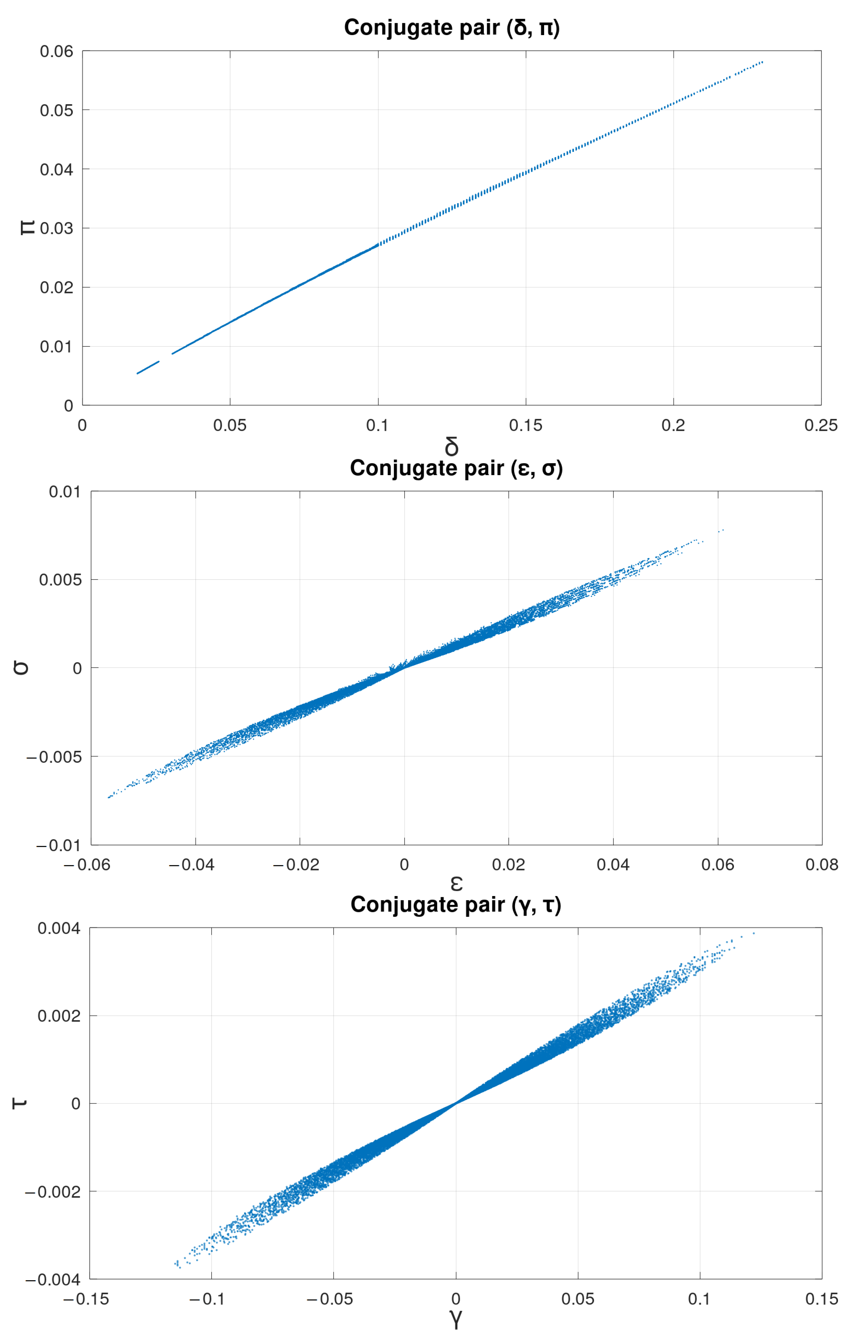
Figure 1. Virtual inflation of the neo-Hookean membrane (26). Top: ( δ , π ) pair; middle: ( ϵ , σ ) pair; bottom: ( γ , τ ) pair. Units of π , σ , τ are Pa·mm. The gap at the beginning is due to elimination of near-boundary triangles from the plots.
Mathematics 10 04447 g001
Figure 2. Virtual inflation of the neo-Hookean membrane (26). Top: ( ϵ , σ ) pair; bottom: ( γ , τ ) pair.
Mathematics 10 04447 g002
Publisher’s Note: MDPI stays neutral with regard to jurisdictional claims in published maps and institutional affiliations.