Abstract
Automated storage/retrieval systems (AS/RS) have been increasingly used to support operations in manufacturing firms, warehouses, and distribution centers. Usually, AS/RSs are expensive. To achieve a good return on investment (ROI), an AS/RS must operate optimally. This research focuses on solving the crane scheduling problem, which has a great and immediate impact on the performance of an AS/RS. To optimize the design and operations of an AS/RS, many past studies have applied the simulation approach. However, the simulation and optimization have been often loosely coupled, resulting in a rigorous and labor-intensive optimization procedure. Using population- and evolution-based metaheuristics to deal with the crane scheduling problem of an AS/RS is one of the research trends. However, the whale optimization algorithm (WOA) and its variants have not been used for this purpose. To address the said gaps, this research first proposes a framework for coupling the simulation and optimization closely, in which various heuristics/metaheuristics, including first-come first-serve (FCFS), RANDOM, WOA, genetic algorithms (GAs), particle swarm optimization (PSO), and especially an improved WOA (IWOA), together with dynamic programming (DP), have been used as alternative sequencing methods. Based on this framework, different simulation-based optimization approaches have been developed for solving the dual-command crane scheduling problem in a unit-load double-deep AS/RS. The experimental results show that IWOA+DP outperforms the others in terms of energy consumption.
Keywords:
automated storage and retrieval (AS/RS); metaheuristics; whale optimization algorithm (WOA); crane scheduling problem MSC:
68U35; 46N20; 74P05; 78M50
1. Introduction
Since the 1950s, automated storage/retrieval systems (AS/RSs) have been increasingly used for material handling in manufacturing firms, warehouses, and distribution centers [1]. The popularity of AS/RSs comes from their advantages, such as high throughput, space-saving ability, high reliability, low inventory cost, and low labor cost [2,3]. An AS/RS is very useful. It can be used to move and accommodate different stock units (SKUs), such as raw materials, work-in-process goods, and finished goods. Usually, AS/RSs are expensive. To have a good return on investment (ROI), an AS/RS must operate optimally.
An AS/RS is composed of hardware and software components that determine the overall performance. The common hardware components of an AS/RS include racks, storage bins, cranes, input/output stations (I/O stations), and a computer. However, software components such as storage and retrieval rules (S/R rules) and storage allocation policies are essential for controlling and using the hardware components of an AS/RS.
For an AS/RS to operate optimally, it needs to deal with relevant problems, including layout, dwell-point location, storage location allocation, batching, and crane scheduling [4]. The first three are long-term problems while the last two are short-term problems. The layout of an AS/RS has a fundamental impact on the AS/RS, which is difficult to change. The dwell-point problem, which involves arranging a place for a crane to stay and wait for the next task, can be considered a part of the layout. Given the layout of an AS/RS, the allocation of storage positions for stocks is another essential long-term problem. Each kind of SKU in an AS/RS can have one/multiple dedicated/open storage position(s). In terms of the short-term problem, the batching problem considers how multiple orders (requests) be combined into one single tour for a human picker or one command cycle for an automated picking device (such as the crane). However, a crane usually has few/no batching options due to limited capacity (one or two shuttles). Another short-term problem, the crane scheduling problem, considers how the storage and retrieval requests can be arranged for a crane. It has an immediate impact on an AS/RS. The performance of a crane is also affected by the command mode used. Single-command and dual-command modes are two common command modes used by a crane. The single-command mode accomplishes one storage or retrieval request within one command cycle while the dual-command mode can complete one storage request and one retrieval request within one cycle. The dual-command mode is advantageous in terms of travel times [5]. A reduction of about 50% of the travel time or an increment of 10-15% of the throughput is possible [6]. Thus, the dual-command mode is focused on in this research. The crane scheduling problem of an AS/RS can be considered a Chebyshev traveling salesman problem, which is known to be NP-complete [7].
Our literature review shows that analytical models, heuristics, metaheuristics, and simulation have been commonly used to deal with crane scheduling problems in an AS/RS. The analytical models have been applied for different kinds of AS/RSs, including unit-load AS/RSs [8,9,10,11,12,13], end-of-aisle mini-load AS/RSs [7,14,15,16], and man-on-board AS/RSs [17]. Heuristics are another commonly used method. Sarker et al. [18] used a simple nearest-neighbor heuristic and a perimeter heuristic to sequence storage and retrieval requests in a dual-shuttle AS/RS. Mahajan et al. [19] proposed a nearest-neighbor heuristic to form dual commands. The heuristic methods were used to solve the crane scheduling problem for man-on-board AS/RSs [20,21,22].
Besides the analytical models and heuristics, population- and evolution-based metaheuristics have been increasingly used to deal with AS/RS problems. Such metaheuristics can improve solution quality through the use of a population of agents and an iterative mechanism. To deal with the crane scheduling problem, Yang et al. [23] used a hybrid genetic algorithm (HGA) for a multi-shuttle AS/RS. The objective was to minimize the travel time needed to complete all storage and retrieval operations. Wu et al. [24] scheduled retrieval requests for a double-deep AS/RS in a flexible manufacturing system. A genetic algorithm (GA), immune GA (IGA), and particle swarm optimization (PSO) were investigated. The objective was to minimize the retrieval time. The IGA was found to be the best in terms of travel distance while the PSO was the best in terms of computational cost. Popović et al. [25] used a GA to sequence requests in a triple-shuttle AS/RS, which used a class-based storage system under a modified sextuple command cycle policy with a planning horizon that comprises the realization of several successive cycles of the S/R machine. Brezovnik et al. [26] optimized AS/RS operations by using an ant colony optimization (ACO) metaheuristic, taking the factor of inquiry (FOI), product height (PH), storage space usage (SSU), and path to dispatch (PD) into consideration. Nia et al. [27] also employed ACO to find a near-optimal solution. The objective was to minimize the total cost of GHG efficiency for the dual-command crane scheduling problem in a unit-load multiple-rack AS/RS. ACO was found to be better than the GA. Chen et al. [28] hybridized ACO with a GA to deal with the routing problem of the crane in a multiple-block warehouse with ultranarrow aisles and access restrictions. Simulations have been used to evaluate 12 warehouse layouts. The experimental results show the superiority of the proposed approach over the dedicated heuristics in terms of solution quality. Cunkas and Ozer [29] used PSO to optimize location assignments for SKUs in a unit-load dual-shuttle AS/RS. The quadruple-command cycle was used. PSO was found to outperform the binary-coded GA (BGA) and real-coded GA (RGA). Tostani et al. [30] proposed a modified cooperative coevolutionary algorithm (MCoBRA) to deal with the dual-shuttle crane scheduling problem in an AS/RS. A bi-level optimization model considering total cost and energy consumption was proposed. The upper level determines the locations of SKUs based on a class-based storage policy. The lower level focuses on solving the crane scheduling problem. Hojaghani et al. [31] formulated a novel mixed-integer nonlinear program (MINLP) for online order batching. The aim was to improve the response and idle times. However, the MINLP was solved by two metaheuristics, ACO and artificial bee colony (ABC), and due to NP-hard, ACO was found better than the ABC. The above literature shows that using metaheuristics to solve the crane scheduling problem is a current trend. However, the whale optimization algorithm (WOA) has never been used for this purpose. Proposed by Mirjalili and Lewis [32], the WOA is a new swarm-intelligence (SI)-based metaheuristic that models the hunting behavior of humpback whales. This algorithm is found to have advantages such as a simple structure, fewer operators, a fast convergence speed, and balanced exploration and exploitation (Mirjalili and Lewis [32]). However, the standard WOA cannot move a whale adaptively, in addition to lacking the mutating capability to increase solution diversity. This kind of metaheuristics has never been used to deal with the crane scheduling problem in an AS/RS.
Simulation is useful to optimize the design and operations of an AS/RS. However, a thorough simulation study is usually necessary before achieving optimality. Ashayeri et al. [33] used simulation for the optimal design of a unit-load automated warehouse for a large oil company in Belgium. Han et al. [6] applied Monte Carlo simulation to improve the throughput of a unit-load AS/RS. FCFS is used as the sequencing rule. A nearest-neighbor sequencing rule was used as an alternative. Azzi et al. [34] also applied Monte Carlo simulation to estimate the travel time of a unit-load multiple-shuttle AS/RS. Randhawa and Shroff [35] used simulation to examine the effects of sequencing rules on six layout configurations of a unit-load AS/RS with different I/O stations, SKU distribution, rack distribution, etc. Lee [36] used the ARENA simulation software to optimize the number of rail-guided vehicles (RGVs) deployed. Hachemi et al. [37] used simulation to study the dual-command crane scheduling problem in a unit-load multiple-rack AS/RS. The objective was to minimize the travel time. FCFS is used for storage requests while the retrieval requests are gathered by block. Yang et al. [38] examined the joint optimization of the crane scheduling problem and storage location assignment problem in a unit-load multi-shuttle AS/RS. They proposed an effective variable neighborhood search (VNS) algorithm. However, in past studies, the simulation and optimization have been often loosely coupled, resulting in a rigorous and labor-intensive solution procedure. A framework for coupling simulation and optimization closely is thus necessary.
Environmental issues are recent global concerns. Boysen and Stephan [4] highlighted the need for energy-efficient crane scheduling for an AS/RS. Nia et al. [27] conducted a unique study that considered the GHG efficiency when dealing with the dual-command crane scheduling problem. However, there are few such studies, necessitating more research incorporating the energy consumption issue.
This research deals with the dual-command crane scheduling problem in a unit-load double-deep AS/RS. A MILP model is firstly formulated after defining this problem. The objective was to minimize energy consumption. Then, a framework is proposed to couple the simulation and optimization closely. Based on this, various simulation-based optimization approaches have been developed, in which various heuristics/metaheuristics, including FCFS, RANDOM, WOA, GA, PSO, and an improved WOA (IWOA), together with DP, have been used as sequencing methods. The experimental results show that the IWOA outperforms the others.
The contributions of this research are highlighted as follows:
- (1)
- A MILP is formulated for this problem;
- (2)
- A framework is proposed to couple the simulation and optimization closely;
- (3)
- An improved WOA (IWOA) with features of adaptive movement and mutation is developed for solving discrete problems using discrete operators;
- (4)
- Experiments are conducted to investigate the effectiveness of different simulation-based optimization approaches;
- (5)
- The successful application of the proposed approaches to solve the dual-command crane scheduling problem in the unit-load double-deep AS/RS is carried out.
The rest of this paper is organized as follows: Section 2 reviews background information on an AS/RS; Section 3 first defines the problem and then formulates a MILP model; Section 4 proposes a simulation-based optimization framework and develops an improved WOA (IWOA) as a sequencing method; Section 5 conducts experiments and analyzes the results; Section 6 presents conclusions and suggestions for the future.
2. Background
2.1. The Common Components of an AS/RS
As shown in Figure 1, an AS/RS includes hardware and software components, which are introduced as follows.
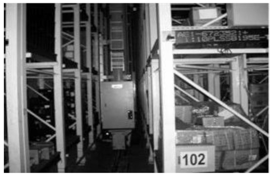
Figure 1.
A single-aisle/double-rack AS/RS.
- (1)
- Hardware components:
- Rack: a mainframe structure used to create a three-dimension space for the accommodation of SKUs. It is the main hardware component of an AS/RS. Each rack is assigned a rack number for identification. A rack can be designed with single, dual, or multiple depths.
- Bin: a cell or basic storage unit partitioned from a rack for storing stock items. Each bin is assigned a bin number for identification or can be identified by a coordinate denoted as (x, y, z), where the x indicates a column number, y indicates a tier number, and z indicates a depth number.
- Aisle: a lane used to separate racks and provide moving space for a crane to reach a target bin position in a rack.
- Crane: also known as storage/retrieval (S/R) machine which is the main device to transport and store/retrieve SKUs into/from the rack of an AS/RS.
- Shuttles: a mechanical device on a crane for transferring SKUs between the crane and rack. A crane can have one, dual, or multiple shuttles, which affects the batching capability of a crane.
- I/O station: a loading/unloading station used to store/retrieve SKUs into/from the AS/RS. In this research, the I/O station defaults as the dwelling point of the crane.
- Computer: a device receiving service requests and controlling the operations of the cranes in the AS/RS.
- (2)
- Software components
Besides the hardware components, the software components are essential for managing and controlling the hardware of an AS/RS. They include:
- Storage rule: a simple rule which decides the storage position or sequence of an SKU. For example, FCFS decides that the earliest arriving SKU should be stored first.
- Retrieval rule: a simple rule which decides the retrieval position or sequence of an SKU. For example, first-in first-out (FIFO) determines that the SKU with the earliest arrival should be retrieved first.
- Scheduling method: a method used to determine the sequences of requested services for a crane. A simple storage rule such as FCFS or Random can be used to schedule the storage requests. However, more comprehensive approaches, such as metaheuristics and simulation, can be used to achieve a more efficient schedule for a crane.
- Zoning policy: a policy arranging available storage space for various kinds of SKUs in an AS/RS. The overall storage space of an AS/RS can be classified into different zones for storing different kinds of SKUs based on their characteristics, such as value or frequency of usage of the SKUs, etc.
- Command mode: a command mode can affect the behavior of a crane. Single-command, dual-command, and multiple-command modes are different command modes of a crane.
- Batching: a method for combining multiple service requests into one tour of service by a picker or a crane.
2.2. The Classification of AS/RS
To solve an AS/RS problem, one first needs to understand the essence of the AS/RS. Referring to Roodbergen and Vis [39], Figure 2 shows a classification scheme based on the attributes of the crane, handling, and rack of AS/RSs. Considering the “shuttle” attribute, a crane can have one single, dual, or multiple shuttles. Considering the “movement” attribute, a cane can be “aisle dedicated” or “aisle shareable” between aisles. Considering the “handling” attribute, an AS/RS can have three types: man-on-board (MOB), end-of-aisle (EOA), and unit-load (UL). The MOB AS/RS has a man on board to pick up SKUs; the EOA AS/RS allows SKUs to be picked up at the end of an aisle; the UL AS/RS accesses the SKUs in pallet or bin units. Considering the “mobility” attribute, a rack can be a “stationary” or “moveable” one. The stationary rack can be “single-deep” or “double-deep.” A movable rack can be the “rotate” or “mobile” kind. The former kind allows rotation in the “horizontal” or “vertical” direction while the latter kind can move in various ways. For example, Kiva robots are used in the Amazon warehouse to move racks.
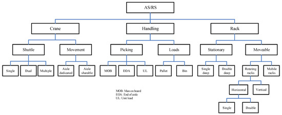
Figure 2.
A classification scheme of AS/RSs.
2.3. Operational Time Analysis for a Dual-Command Crane in a Unit-Load Double-Deep AS/RS
Figure 3 shows the moving paths a crane uses to complete a dual command. First, the crane performs the storage request i by moving from the I/O station to the storage position S1, (,,) This travel time is denoted as T1. Then, the crane performs the retrieval request by moving from position S1 to position R1, (,,). This travel time is denoted as T2. Finally, the crane moves the retrieved SKU back to the I/O station. The travel time of the last movement is denoted as T3. The total time to complete this dual command is formulated as Equation (1).
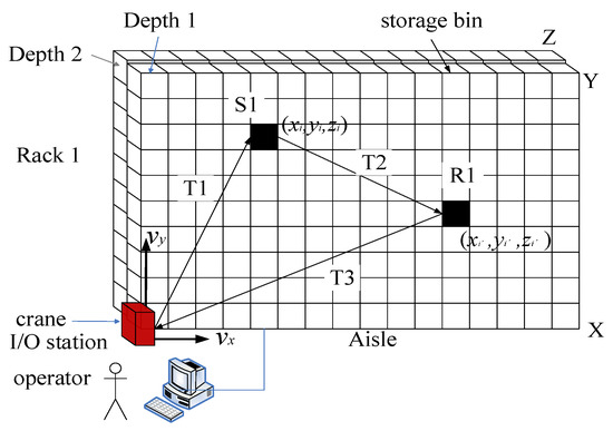
Figure 3.
A unit-load and double-deep AS/RS.
(meter/second) is the moving speed of the crane along the horizontal direction while (meter/second) is the moving speed of the crane along the vertical direction. W and H indicate the width and height (in the unit of meters) of each storage bin, respectively.
ts is the time needed for the shuttle to store the SKU on a rack. This time is affected by the depth of the storage position of the SKU to be stored. Thus, ts is estimated by Equation (2).
D indicates the depth of a storage position in a rack. is the moving speed of the shutter along the Z direction. Cs is a coefficient for extending the storage time required for the SKU assigned at the second depth (i.e., in a rack.
tr is the time needed for the shuttle to retrieve an SKU from a rack. Additionally, this time can be affected by the storage depth of the SKU in the rack. It is estimated by Equation (3).
The Cr is a coefficient for extending the retrieval time required for the SKU stored at the second depth (i.e., in a rack.
2.4. Energy Consumption Calculation
Based on Nia et al. [27], the tax cost of energy consumption for the crane is calculated by Equation (4).
where:
power consumption of crane (k watts/second);
GHG conversion factor;
GHG emission cost.
The penalty cost of exceeding GHG emissions and the discount for producing less GHG emissions than expected are not taken into account in this research.
3. Problem Definition and Mathematical Model Formulation
3.1. Definition of the Dual-Command Crane Scheduling Problem
In this research, dual-command crane scheduling is defined as a problem of forming the storage and retrieval service requests into dual-commands and sequencing their execution orders for a crane in a unit-load and double-deep AS/RS. Each crane is dedicated to serving two racks on both sides of a specific aisle. The racks have double the depth, i.e., double-deep racks (as shown in Figure 3). The crane moves in the horizontal and vertical directions simultaneously, with the moving distance measured by the Chebychev metric. Based on the classification notation proposed by Boysen and Stephan [4], this problem is denoted as
where:
F: I/O station at the front end;
Open: any open shelf is a potential location for storage requests;
: double commands;
: the total cost of energy consumption for the crane using a dual command (storage request i and retrieval request ). This is a new objective function.
The objective considers the total energy consumption cost of the crane.
Figure 4 represents a solution to this problem. The SR and RR are the sequences of storage and retrieval service requests, respectively. The parameter N = 10 indicates the total number of dual commands of storage and retrieval service requests. In this solution, the dual command of storage and retrieval requests is executed in the following sequence: (5,2),(3,6),(4,1),(1,10),(7,7),(2,4),(9,8),(6,5),(8,3),(10,9). If the storage and retrieval requests are sequenced according to their arrival times, then this is a solution obtained from the FCFS rule. Each dual command is executed by the crane with the schedule [], where and are the start and end times, respectively.
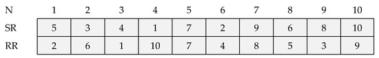
Figure 4.
The representation of sequences of storage requests (SRs) and retrieval requests (RRs).
3.2. Mathematical Model Formulation
This section focuses on formulating a mathematical model for the dual-command crane scheduling problem. Before doing this, the required assumptions, indices, sets, parameters, and decision variables are first defined as follows.
- Assumptions:
- Each storage/retrieval request is associated with one SKU.
- The position (x,y,z) of each SKU to be stored/retrieved is specified in each storage/retrieval request.
- The crane moves in the X (horizontal) and Y (vertical) directions simultaneously and the distance is measured by the Chebychev metric.
- No interruption occurs during the transport, storage, and retrieval operations.
- There are N storage and N retrieval requests to be handled by a specific crane.
The indices, sets, parameters, and decision variables required for the MILP are defined as follows.
- Indices:
| i, j , r x y z | a storage request ID; i, j; a retrieval request ID; , ; a rack number; r ; a column number on a rack; x ; a tier number on a rack; y ; a deep number on a rack; z . |
- Sets:
| SR RR R X Y Z | a set of storage requests;; a set of retrieval requests;; a set of rack; R ; a set of columns; X ; a set of tiers on a rack; Y ; a set of depth numbers; Z . |
- Parameters (Input data):
| the number of racks served by a crane; | |
| the total number of columns of a rack; | |
| the total number of tiers of a rack; | |
| the total number of depths in a rack; = 1 (1st depth); = 2 (2nd depth) | |
| the total number of storage/retrieval service requests | |
| (,, | the storage position of an SKU i in a rack; |
| (, | the storage position of an SKU in a rack; |
| the moving speed of a crane along the X horizontal (column) direction; | |
| the moving speed of a crane along the Y vertical (tier) direction; | |
| the moving speed of a shuttle along the Z (depth) direction; | |
| the shuttle time to store an SKU into the AS/RS; | |
| the shuttle time to retrieve an SKU from the AS/RS; | |
| GHG conversion rate; | |
| penalty cost of GHG emissions; | |
| a coefficient extending the storage time required for the SKU which is to be stored in the second depth in the rack; | |
| . | a coefficient extending the retrieval time required for an SKU stored in the second depth in a rack. |
- Decision variables:
| , if the storage request i is performed before the storage request j; , otherwise; | |
| , if the retrieval request is performed before the retrieval request ; , otherwise; | |
| , if the storage request i and the retrieval request is a pair of dual-command; , otherwise. |
A sequence of dual commands of storage and retrieval requests is to be created. The MILP model for the crane scheduling problem is formulated as follows:
s.t.
Equation (5) is the objective function of minimizing the total cost of energy consumption of the crane. Equations (1)(4) are also included. Constraint (6) defines the condition for the variable . Constraints (7)(10) relate to the variables Constraint (7) ensures that each storage request has only one predecessor. Constraint (8) ensures each storage request has only one successor. Constraints (9)(10) relate to the variable which assigns a sequence of storage requests from a network view. Constraint (9) states that on leaving node i, there are no more than N − 1 remaining storage requests to be assigned. Equation (10) is a conservation constraint for node i. Similarly, constraints (11) and (14) relate to the variable . Constraint (11) ensures that each retrieval request has only one predecessor. Constraint (12) ensures each retrieval request has only one successor. Constraints (13)(14) are associated with the variable , which assigns retrieval requests from a network view. Constraint (13) states that on leaving node , there are no more than N − 1 remaining retrieval requests to be assigned. Equation (14) is a conservation constraint for node . Constraints (15)(17) are associated with the variable Constraint (15) ensures there are exactly N pairs of dual commands. Constraint (16) ensures that a retrieval request is assigned with one storage request only. Constraint (17) ensures that a storage request is assigned with one retrieval request only. Constraint (18) stipulates that , and are binary variables.
This problem has a solution space of N!N!, which tends to become computationally intractable if the N is big enough. Thus, a simulation-based optimization approach is proposed as an alternative approach.
4. Simulation-Based Optimization Approaches
4.1. A Simulation-Based Optimization Framework
Due to NP-complete, this section proposes a framework (Figure 5) that couples the simulation and optimization closely for developing alternative simulation-based optimization approaches. The main layers/functions of this framework are introduced as follows:
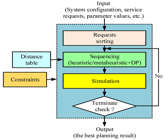
Figure 5.
The simulation-based optimization framework.
- Input: this is an initial step to creating input data for experiments. Configuration data of the AS/RS, such as the number of racks, the dimension of a rack, the moving speed of the crane, and the parameter values of heuristics/metaheuristics, are set manually. On the other hand, the storage and retrieval requests of SKUs and their target positions (x,y,z) are generated by a computer automatically. This simulates the randomness of service requests in the real world.
- Requests sorting layer: this layer sorts out the storage and retrieval service requests specifically for each crane based on the SKU’s positions. Since the SKUs to be stored/retrieved are distributed across racks in the AS/RS, it needs first to sort out the storage and retrieval requests for each crane. As said previously, each crane is dedicated to serving two specific racks on both sides of an aisle. The sorting is based on the rack positions of the target SKUs. The storage and retrieval requests specifically for each crane are inputted to the sequencing layer.
- Sequencing layer: this layer focuses on generating alternative sequences of dual commands (one storage and one retrieval request) for a crane. Two simple heuristics (Random and FCFS) and four metaheuristics (WOA, IWOA+DP, GA, and PSO) are used in this research to generate and sequence dual commands. Conversely, the IWOA+DP uses a two-stage procedure. First, the IWOA finds a sequence of storage requests, based on which the dynamic programming (DP) method (detailed in Section 4.4) is used in the second stage to assign each storage request a retrieval request to become a dual command. The sequence of dual commands is inputted into the simulation layer. As each sequence of storage and retrieval requests is NP-complete, the use of an analytical model to solve this problem optimality tends to become computationally intractable.
- Simulation layer: with the sequence of dual commands as input, this layer simulates the crane operations and evaluates the results. The best solution can be identified in this layer.
- Termination check: a check function is used to check whether the stop condition is reached. A total number of iterations is used as a stop condition in this research.
- Output: this step outputs the best solution.
The framework can be transformed into a workflow diagram with input and output data flows represented as dotted red arrow lines, as shown in Figure 6. For example, the Simulation module inputs distance data of each dual command into the Energy calculation modulem which calculates and returns the energy cost of dual commands.
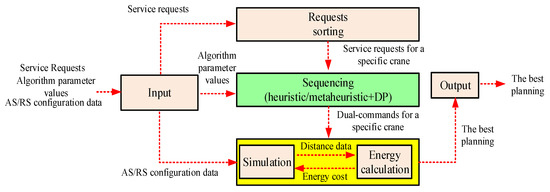
Figure 6.
The workflow diagram of modules with input and output data flows.
4.2. Position Scheme
Figure 7 shows the position scheme of whales to search for a solution space. It includes two segments, each with the dimension N, where N is the total number of storage/retrieval requests.
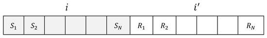
Figure 7.
The position scheme used by whales.
The left segment represents the sequence of storage requests, in which indicates the order of the storage request i (i [1, N]). The right segment indicates the sequence of retrieval requests, in which indicates the order of the retrieval request ( [1, N]). A series of dual commands are then formed and represented as (,), where i [1, N].
4.3. WOA and Improved WOA (IWOA)
The WOA and IWOA are further detailed as follows.
4.3.1. WOA
Figure 8 shows the spiral-shaped movement of whales when they are circling and attacking their prey. Each whale’s position represents a solution in the solution space. Then, the distance between a whale and the prey (fish schools) represents an objective function value. The aim is to minimize the distance. The whales change their positions continuously during the hunting process, which contains three phases: encircling, prey, bubble-net attack (exploitation phase), and the search for prey (exploration phase) [32].
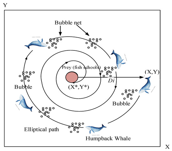
Figure 8.
The spiral movements of humpback whales when hunting prey.
- (1)
- Encircling prey
After noting the prey (school fish), the humpback whales set out to encircle and attack them. However, not knowing the prey’s exact position, it is assumed that the global best whale is closest to the prey. Equation (19) shows the distance between the whale i and the target prey.
and are position vectors of the whale i and the global best whale respectively. is a coefficient vector defined by Equation (20).
[0,1] is a vector of random numbers. Given the distance , the next position of the whale i is determined by Equation (21).
is a coefficient vector defined by Equation (22).
where the is a linear value decreasing from 2 to 0 iteratively.
- (2)
- Bubble-net attack (exploitation phase)
Equation (23) defines the use of shrinking circle- or spiral-shaped paths for whales during the exploitation phase.
The parameter random number p [0,1] controls the selection of the shrinking circle- or spiral-shaped path. If , then the shrinking circle is used; otherwise, the spiral-shaped path is used. The parameter b (a constant value) defines the shape of the logarithmic spiral. The parameter l [0,1] is a random number.
- (3)
- Search for prey (exploration phase)
controls the use of either an exploration or exploitation search for a whale. If 1, Equations (24) and (25) are used for the exploration search.
is the position of a randomly selected whale. If 1, then replace in Equations (24) and (25) with for the exploitation search.
Figure 9 shows the workflow of Algorithm A1 of the WOA. Appendix A shows the pseudo-code of the WOA.
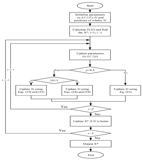
Figure 9.
The workflow of Algorithm A1 of the WOA.
4.3.2. Improved WOA (IWOA)
The IWOA allows the humpback whales to be guided by a set of elite whales (denoted as ES), instead of only the global best whale . Whale i can develop adaptive steps by referring to an elite whale ES.
- Adaptive movement of whales:
Referring to an elite whale , whale i develops an adaptive movement through the following three steps:
(1) Determine the Hamming distance: the first step is measuring the Hamming distance between the whale i and the elite whale , based on their current position vectors.
The Hamming distance is defined in Equation (26).
It counts the total number of different elements between the two position vectors and , where the D is a dimension of the vectors. and are the i-th elements in and , respectively. The XOR is an operator leading to either 1 () or 0 ().
(2) Determine a change rate (CR): the CR is a change rate controlling the replacement of the k-th element in (t+1) with the k-th element in simulating the movement toward the . A whale that is farther out requires a bigger CR, as defined in Equation (27).
(3) Determine the next position of the whale i:
Based on the CR, this step determines the k-th element in the next position of whale i using Equation (28).
[0, 1] is a random number used for determining the k-th element in (t + 1). Equation (28) provides a whale that is farther out with a higher opportunity to make a bigger step, while a closer whale is more likely to make a smaller step toward the . However, if replaces in , will take the place of the original to ensure a feasible solution.
For example, given that [5,4,3,2,1] and = [3,4,2,5,1] are the current positions of the whale i and the elite whale respectively, then we can derive HD(i,) = 2, CR = 3/5 = 0.6. Additionally, the next position vector of the whale i will be determined by Equation (28). Given the random number = 0.5, then becomes 3, and element 5 in will take the position of 3 in and appear in . Note that the derived solution remains feasible.
In addition, the IWOA includes the following features:
- The use of Sobol sequence:
This Sobol sequence enables the IWOA to initialize more uniform-distributed positions of whales in the solution space through the use of Sobol sequence numbers [40]. One weakness found in many past studies is that the random numbers generated by pseudorandom number generators embedded in the standard libraries of programming languages are not uniformly distributed [41].
- Mutation:
Mutation can diversify solutions. It avoids solutions sticking to local optima. Thus, the IWOA introduces a mutation( ) procedure that includes two kinds of mutations, swap mutation (SM) and inverse mutation (IM).
(1) Swap mutation (SM): this is a mutation that switches elements at two randomly selected points (such as p1 and p2) in a vector. For example, given p1 = 2 and p2 = 6, the position vector [71324586] is mutated to [75324186].
(2) Inverse mutation (IM): this mutation mutates elements in reverse order between two randomly selected points (p1 and p2) in a vector. The IM can have a higher degree of mutation. For example, given p1 = 2 and p2 = 6, the position vector [71324586] is mutated to [75423186]. The IM has a bigger range of mutations.
Based on Hamming distance, a similarity degree (SD), as defined in Equation (29), is used to determine the use of SM or IM.
HD(, ) is defined in Equation (26).
Figure 10 shows the workflow of Algorithm A2 of the procedure mutation( ). Appendix B shows the pseudo-code. The mutation happens when the condition, R1 < , is true. R1 and [0,1], represent a random number and a mutation rate, respectively. The values of SD and control the use of either IM or SM. If SD < then the IM is used; otherwise, the SM is used. The smaller the , the lower the probability of using the IM. A solution remains feasible after mutation due to a combination of sequence numbers from 1 to N.
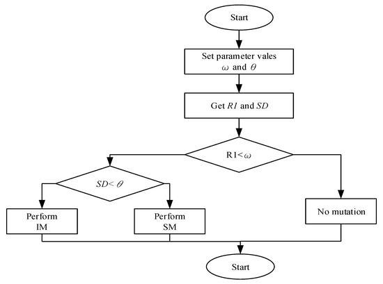
Figure 10.
The workflow of Algorithm A2 of the procedure mutation( ).
4.4. The Dynamic Programming
The DP works together with the IWOA to form a sequence of dual commands. With the output obtained from the IWOA in the first stage (i.e., the sequence of storage requests), the forward DP is used to form a sequence of dual commands by assigning each storage request with a retrieval service request through the N stages. The DP model contains Equations (30)–(32).
At each stage k (k = 1, …, N), the DP model assigns each storage request with a retrieval request at the k order, based on the distance table. In Equation (30), indicates the total retrieval distance at stage 1; is the minimum distance at the state j of Stage 1, transitioned from the state s of the dummy stage 0; is a set of available states at Stage 1. In Equation (31), the indicates the total retrieval distance at Stage k. is the minimum distance at state j of Stage k, transitioned from the state i of Stage k-1, where 2. indicates the set of available states at Stage k. In Equation (32), indicates the total retrieval distance at the final Stage N. indicates the total retrieval distance at state j of the final Stage N transitioned from the state i at the previous Stage . The indicates the set of available states at Stage N. At each stage k (1), the DP forms a dual command consisting of one storage and one retrieval request.
4.5. The Main Logic Flow of the IWOA
Figure 11 shows the workflow of Algorithm A3 of the IWOA. Appendix C shows the pseudo-code. Compared with Algorithm A1, line 3 changes to using a Sobol sequence generator to initialize positions for whales; lines 8–19 include an additional loop, where NE is the number of elites in the elite set ES; line 11, 14, and 17 change to use adaptive movements for whales; and line 24 adds a mutation procedure, mutation( ). These are new features in the IWOA.
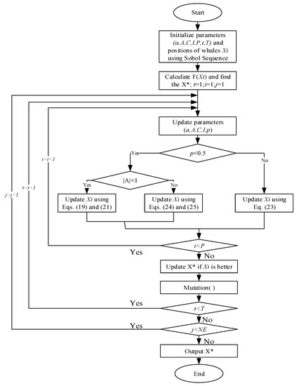
Figure 11.
The workflow of Algorithm A3 of the IWOA.
4.6. Simulation Model
Figure 12 shows a timed predicate/transition net as a discrete-event simulation model for dealing with the dual-command crane scheduling problem. The main components of a timed predicate/transition net include the predicate, transition, and directed arc [42,43]). They are defined as follows:
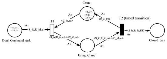
Figure 12.
A discrete-event simulation model of timed predicate/transition net.
- Predicate = {Dual_Command_task, Crane, Using_Crane, Closed_task};
- Transition = {T1,T2};
- Arc = {A1, …, A6}.
Each predicate accompanied by a circle symbol asserts a fact. For example, the Dual_commnd_task predicate asserts the truth/false of the existence of dual-command task(s). It becomes true once a task token <S_id,R_id,ai> appears in the corresponding circle symbol. The token’s attributes correspond to the storage_request_id, retrieval_request_id, and available_time of the request I, respectively. The Crane predicate asserts the truth/false of the existence of available crane(s). It becomes true once a crane token <C_id,> appears in the corresponding circle symbol. The token’s attributes correspond to the crane_id and available_time of the crane c, respectively. The predicate Closed_task asserts the truth/false of the existence of completed task(s). It becomes true whenever a task token appears in the corresponding circle symbol. T1 and T2 are transitions that are represented by bar symbols. Transition T1 is “firable” when both the Dual_Command_task and Crane predicates become true simultaneously. T2 is firable once a combined token <S_id,R_id,ai>+<C_id,> appears in the Using_Crane predicate. T2 is a timed transition as it takes time to complete the transition. After this transition, the crane token <C_id,ET> is returned to the Crane predicate; meanwhile, the task token <S_id,R_id,ET) is transitioned to the Closing_task predicate. When all tokens stay with the Closing_task predicate, the simulation stops running.
Let and be the available times of the SKU i (i T) and the crane c, respectively. Then, the start time of handling the i-th paired requests () is determined by Equation (33).
Let be the travel time for this pair of storage and retrieval requests. Equation (34) is used to estimate the completion time.
5. Numerical Experiments
This section evaluates the effectiveness of FCFS, RANDOM, GA, PSO, WOA, and IWOA+DP used as sequencing methods in the simulation-based optimization framework. First, a small-size instance is used to demonstrate the result. Then, extensive experiments are used to conduct a thorough evaluation. These experiments were performed on a computer with Intel PENTIUM CPU 2117U (64 bits and 1.8 GHz) and 4 GB DRAMs. Java was used as the programming language to implement these approaches.
5.1. Parameter Value Settings for Experiments
After sorting out the requests, the requests for SKUs to be handled on a specific crane will be found. For experiments, we set the number of cranes to one and the number of racks to two (R = {1, 2}, where the R is a set of racks served by the crane). Referring to Nia et al. [27],= 4 (meters/s), = 0.9 (meters/s), = 4 (meters/s), = 1172 (k W/s), = 0.1, and = 1.508 are used. In addition, we set the dimension of each rack to be (X, Y,Z) = (40,30,2), indicating that there are 40 × 30 × 2 storage bins. The dimensions of each bin are: W = 1.15 m (width), H = 1.32 m (height), and D = 1.5 m (depth). For the SKUs at the second depth of a rack, parameter values == 2.5 are used.
Table 1 shows the parameter values set for different approaches, in which N indicates the total number of storage/retrieval requests; P indicates the total number of individuals in the population; I indicates the total number of iterations; indicates the upper limit of velocity; indicates the lower limit of velocity; Rm indicates a mutation rate for GA; Rc indicates a crossover rate for the GA; indicates the mutation rate for the IWOA; indicates the threshold for using IM or SM; NE indicates the number of elites in the elite set ES; - indicates not used.

Table 1.
The parameter setting for different approaches.
5.2. Experimental Instance Generation
Based on the parameter value settings, a computer is used to generate random storage and request services. This simulates the randomness of real operations. A total number of N storage and retrieval requests of SKUs and the target position of these SKUs are generated. The problem size is defined as NN.
5.3. An Example of a Small Instance
A small-sized experimental instance (N × N = 15 × 15) is used to illustrate the obtained results.
Based on the parameter values (X,Y,Z) = (40,30,2) and RK = {1,2} set in Section A, experimental instances are automatically generated by the computer for experiments. Table 2a,b show the storage and retrieval requests automatically generated by the computer, respectively. In the two tables, S_id indicates a storage request ID; R_id indicates a retrieval request ID; r indicates a rack number r R; x indicates a column number; y indicates a tier number; z indicates a depth number of an SKU.
Table 2.
(a). The storage requests (N = 15). (b). The retrieval requests (N = 15).
Different approaches are then used to find the best solution. Table 3a–f show the experimental results obtained by (a) FCFS, (b) RANDOM, (c) the WOA, (d) the GA, (e) PSO, and (f) the IWOA+DP.
Table 3.
(a). The best solution found by FCFS (problem size: N × N = 15 × 15). (b). The best solution found by RANDOM (problem size: N × N = 15 × 15). (c). The best solution found by WOA (problem size: N × N = 15 × 15). (d). The best solution found by GA (problem size: N × N = 15 × 15). (e). The best solution found by PSO (problem size: N × N = 15 × 15). (f). The best solution found by the IWOA+DP (problem size: N × N = 15 × 15).
In Table 3(a–f), S_id indicates a storage request ID; R_id indicates a retrieval request ID; T1 indicates the travel time to the storage location; it indicates the storage shuttle time; T2 indicates the travel time from the storage location to the retrieval location; tr indicates the retrieval shuttle time; T3 indicates the travel time from the retrieval location to the I/O station; T(DC) indicates the total process time of each dual command; TPT indicates the accumulated total time of this sequence of dual commands.
Table 4 summarizes the experimental results. It is found that the IWOA finds the best solution with Z = 1.63E+10 at the computation cost of 3.476 s. The WOA finds the best solution with Z = 1.76E+10 at the computation cost of 2.26 s; the PSO finds the best solution with Z = 1.72+10 at the computation cost of 2.25 s; the GA finds the solution with Z = 1.78E+10 at the computation cost of 1.78 s; the Random heuristic finds the best solution with Z = 1.80E+10 at the computation cost of 1.98 s; the FCFS finds the best solution with Z = 1.81E+10 at the computation cost of 0.06 s. This case shows that the IWOA outperforms the others in terms of Z value.
Table 4.
The summary of different approaches.
5.4. Extensive Experiments using Different Problem Sizes
Extensive experiments using different problem sizes have been further conducted to investigate the effectiveness of different approaches. Table 5 shows the experimental results, which are summarized are follows:
Table 5.
The results obtained from different approaches using different problem sizes.
- At the problem size 50 × 50, the IWOA+DP has average edges of 16.84%, 17.57%, 17.67%, 18.32%, and 25.38% over the PSO, WOA, GA, RANDOM, and FCFS, respectively. Figure 13 shows the box-whisker plot of the Z values of the problem size 50 × 50 obtained using different approaches.
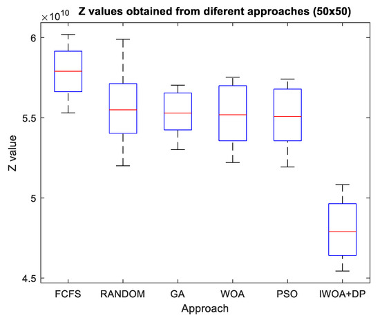 Figure 13. The box-whisker plot chart of Z values found for the problems (50 × 50).
- At the problem size 100 × 100, the IWOA+DP has average edges of 20.55%, 20.05%, 20.45%, 24.08%, and 24.86% over the PSO, WOA, GA, RANDOM, and FCFS, respectively. Figure 14 shows the box-whisker plot of the Z values of the problem size 100 × 100 obtained using different approaches.
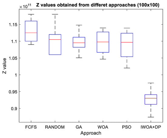 Figure 14. The box-whisker plot chart of Z values found for the problems (100 × 100).
- At the problem size 150 × 150, the IWOA+DP has average edges of 21.43%, 22.78%, 21.92%, 21.98%, and 23.92% over the PSO, WOA, GA, RANDOM, and FCFS, respectively. Figure 15 shows the box-whisker plot of the Z values of the problem size 150 × 150 obtained using different approaches.
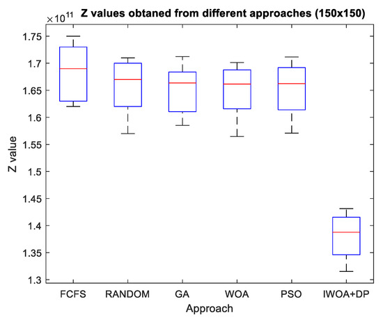 Figure 15. The box-whisker plot chart of Z values found for the problems (150 × 150).
- Experiments with different problem sizes consistently show that IWOA+DP outperforms the other approaches.
5.5. Statistical Tests
At the significance level of α = 0.05, the statistical t-test is used to test Hypotheses H0 and H1, where the H0 assumes that the average Z values of comparing approaches have no significant difference; H1 assumes that these average Z values are different.
Table 6 shows the t-test results of each approach compared to the IWOA. The symbol “+” indicates that the IWOA is better; the symbol “−” indicates that the IWOA is inferior; the symbol “N” indicates no difference. The p-values of these comparisons are found to be less than 0.005. For example, at the problem size N = 100, the p-values of RANDOM, FCFS, the GA, PSO, and the WOA are 2.13695E-11, 1.48414E-09, 2.07195E-11, 5.69295E-09, and 2.08357E-11, respectively. The results lead to the rejection of H0 and the acceptance of H1. Thus, IWOA is confirmed to outperform the others in terms of the statistical t-test.
Table 6.
Results of t-test for different approaches at different problem sizes.
5.6. Analysis and Discussion
- The experiments demonstrate the feasibility of using closely coupled simulation-based optimization approaches to deal with the dual-command crane scheduling problem in a unit-load and double-deep AS/RS. The use of dual commands to operate an AS/RS is not difficult, especially in a busy AS/RS environment. For a high-workload AS/RS, we can set a higher value for N. For a low-workload AS/RS, we can lower the value for the N. The use of dual-command operation is advantageous for a crane.
- On average, metaheuristics have a better performance than simple heuristics (Random and FCFS) in terms of solution quality due to the use of a guided search, instead of a random search.
- In general, the greater the N, the higher the advantage for the IWOA+DP.
- Though other metaheuristics such as GAs, PSO, and FAs are also population- and evolution-based metaheuristics, they cannot outperform the IWOA+DP.
- Metaheuristics in general can achieve a better solution than the heuristics (RANDOM and FCFS) due to the use of an informed search. In contrast, RANDOM uses a kind of random search.
- In this research, the RANDOM outperforms FCFS due to being empowered with an iterative mechanism that gives RANDOM more chances to find a better solution. FCFS is one special case of the RANDOM search. However, the two heuristics cannot outperform the other metaheuristics.
- Though the standard WOA provides an exploration mechanism when |A| 1, this exploration scope is still affected by the whales in the swarm. In the IWOA, a global mutation capability is additionally provided by the mutation( ) procedure. In addition, the IWOA uses an adaptive movement, in addition to working with DP.
- In this research, the GA, WOA, and PSO generate positions for a population with real numbers, and then the ROV technique is used to transform the positions into solutions in the discrete domain of sequence numbers. The transformation procedure is used by these approaches during the whole solution process. However, the IWOA is different. After transforming the initial positions of the whales from the continuous domain to the discrete domain by using the ROV technique, the following evolutions of solutions are based on the discrete operator, as stated in Equations (26)(28). The use of discrete operators appears to result in a better result as the crane scheduling problem is in essence in the discrete domain. Though the ROV transformation procedure is necessary to develop a feasible solution, the use of discrete operators to evolve solutions in a discrete domain appears to lead to a better result.
- Szczepanski et al. [44] highlighted two common ways of handling constraints. One is the inclusion of the penalty function into the objective function and another is the separation of the objective function and constraints. The former decreases the fitness of an infeasible solution so as to find a feasible solution. However, in this research, we use the ROV technique, and this technique can always return feasible solutions to our focused scheduling problem. Thus, there is no need to use the penalty function for constraints in the objective function. The solutions transformed by the ROV techniques are always subject to the constraints described in Section 3.2.
- Several intelligent algorithms have been proposed by researchers to deal with multiple objective optimization problems (MOPs), such as in [45,46,47]. Fountas et al. [45] proposed a virus-evolutionary genetic algorithm (GA) to optimize the tool path parameters in the sculptured surface. This algorithm is a variant of the standard GA. Rahman et al. [46] proposed a multi-objective learner performance-based behavior (MOLPB) algorithm for dealing with real-world engineering optimization problems. Zhang et al. [47] proposed an SDNSGA-III algorithm to deal with the dynamic multi-objective optimization problems (DMOPs) that have dynamic objectives and constraints in a changing environment. Our preliminary survey shows that there is a possibility of comparing the three algorithms with the IWOA proposed in this research if the ROV technique is applied to the three algorithms. This can be treated as a future research direction. In addition, these studies show that a multi-objective function can be used as a performance measurement of a crane in future research.
6. Conclusions
The crane scheduling problem affects the performance of an AS/RS considerably. This research first defines the dual-command crane scheduling problem in a unit-load double-deep AS/RS. Following this, a MILP is formulated for this problem, with the objective of minimizing energy consumption. To couple the simulation and optimization closely, we have proposed a framework for developing simulation-based optimization approaches in which heuristics/metaheuristics, including FCFS, RANDOM, an IWOA, an WOA, a GA, and PSO, have been used as alternative sequencing methods. Experiments have been conducted to investigate their effectiveness. The experimental results show that the IWOA outperforms other heuristics/metaheuristics.
The contributions of this research are summarized as follows: (1) a MILP is formulated for this problem; (2) a framework is proposed to couple the simulation and optimization closely; (3) an improved WOA (IWOA) with features of adaptive movement and mutation is developed for solving discrete problems using a discrete operator; (4) experiments were conducted to investigate the effectiveness of different simulation-based optimization approaches; (5) the successful application of the proposed approaches to solve the dual-command crane scheduling problem in a unit-load double-deep AS/RS.
Future research can focus on the following directions. First, the assumption of the same number of storage and retrieval requests made in this research can be relaxed. Second, other metaheuristics, such as those proposed in [45,46,47], can be compared with multi-objective functions. Third, the allocation policies can be incorporated. Fourth, this approach can be applied to other kinds of AS/RSs. Lee [36] highlighted that AS/RSs are only used as an alternative to traditional systems but are also a part of the manufacturing system to support manufacturing.
Author Contributions
Conceptualization, H.-P.H.; Data curation, H.-P.H.; Formal analysis, C.-N.W.; Funding acquisition, H.-P.H.; Investigation, C.-N.W.; Methodology, H.-P.H.; Project administration, C.-N.W.; Software, H.-P.H.; Validation, T.-T.D.; Writing—original draft, H.-P.H.; Writing—review and editing, T.-T.D. All authors have read and agreed to the published version of the manuscript.
Funding
The authors received no specific funding for this study.
Data Availability Statement
Not applicable.
Acknowledgments
The authors appreciate the support from the National Kaohsiung University of Science and Technology, Taiwan; and Hong Bang International University, Vietnam.
Conflicts of Interest
The authors declare no conflict of interest.
Appendix A
| Algorithm A1. The psudo-code of the WOA |
| Define the problem // for a minimize problem Define the objective function F(X) Set parameter T (total number of iterations) P, and b Initialize the a, A, C, and l Initialize the positions Xi of whales i (i = 1, 2, 3,…, P) Calculate the F(Xi) for each whale i Find the X* REPEAT1 while (t<=T) or (stop criterion) Update a, , , l, and p REPEAT2 while (i<P) IF (p < 0.5) // shrinking circle movement IF (|A| < 1) // exploition Update the Xi using Equations (19) and (21) ELSE (|A| 1) // exploration Select a random XR from the whale group Update the Xi using Equations (24) and (25) ENE IF ELSE // spirial-shaped movement Update the Xi using Equation (23) END IF END REPEAT2 (until I > P) Check if any whale is out of the search space and amend it Evaluate F() for each whale i Update the if better END REPEAT1 (until t>T) Output X* |
Appendix B
| Algorithm A2. The psudo-code of the mutation( ) |
| Set the mutation rate Set the mutation rate // threshold Generate the random variable R1 and R2 If R1 < // perform mutation If SD< Use IM ELSE Use SM ELSE No mutation END IF |
Appendix C
| Algorithm A3. The pseudo-code of the IWOA | |
| 1 | Define the objective function F(X) of the problem |
| 2 | Set parameter T (the total number of iterations); a, A, C, l, and p |
| 3 | Initialize the positions Xi of whales (i = 1, 2, 3,…, N) using Sobol sequence generator |
| 4 | Calculate the F(Xi) for each whale i; and find the ES |
| 5 | REPEAT1 while (t<=T) or (stop criterion) |
| 6 | Update parameters a, , , l, and p |
| 7 | REPEAT2 while (i<=N) |
| 8 | REPEAT3 while (j<=NE) |
| 9 | IF (p < 0.5) |
| 10 | IF (|A| < 1) // Exploitation |
| 11 | Update the Xi using Equations (26)(32) |
| 12 | ELSE (|A| 1) // Exploration |
| 13 | Select a random whale XR from the whale group |
| 14 | Update the Xi using Equations (26)(32) |
| 15 | ENE IF |
| 16 | ELSE |
| 17 | Update the Xi using Equations (26)(32) |
| 18 | END IF |
| 19 | END REPEAT3 (until j > NE) |
| 20 | END REPEAT2 (until i >N) |
| 21 | Check and amend the whales out of the search space |
| 22 | Evaluate F() for each whale i; |
| 23 | Update the if better |
| 24 | Mutation ( ) |
| 25 | END REPEAT1 (until t >T) |
| 26 | Output X* |
References
- Eynan, A.; Rosenblatt, M.J. Establishing Zones In Single-Command Class-Based Rectangular As/Rs. IIE Trans. 1994, 26, 38–46. [Google Scholar] [CrossRef]
- Rosenblatt, M.J.; Roll, Y.; Vered Zyser, D. A Combined Optimization And Simulation Approach For Designing Automated Storage/Retrieval Systems. IIE Trans. 1993, 25, 40–50. [Google Scholar] [CrossRef]
- Hu, Y.-H.; Huang, S.Y.; Chen, C.; Hsu, W.-J.; Toh, A.C.; Loh, C.K.; Song, T. Travel Time Analysis of a New Automated Storage and Retrieval System. Comput. Oper. Res. 2005, 32, 1515–1544. [Google Scholar] [CrossRef]
- Boysen, N.; Stephan, K. A Survey on Single Crane Scheduling in Automated Storage/Retrieval Systems. Eur. J. Oper. Res. 2016, 254, 691–704. [Google Scholar] [CrossRef]
- Graves, S.C.; Hausman, W.H.; Schwarz, L.B. Storage-Retrieval Interleaving in Automatic Warehousing Systems. Manag. Sci. 1977, 23, 935–945. [Google Scholar] [CrossRef]
- Han, M.-H.; McGinnis, L.F.; Shieh, J.S.; White, J.A. On Sequencing Retrievals In An Automated Storage/Retrieval System. IIE Trans. 1987, 19, 56–66. [Google Scholar] [CrossRef]
- Bozer, Y.A.; White, J.A. Design and Performance Models for End-of-Aisle Order Picking Systems. Manag. Sci. 1990, 36, 852–866. [Google Scholar] [CrossRef]
- Karasawa, Y.; Nakayama, H.; Dohi, S. Trade-off Analysis for Optimal Design of Automated Warehouses. Int. J. Syst. Sci. 1980, 11, 567–576. [Google Scholar] [CrossRef]
- Zollinger, H.A. Planning, February, Evaluating, and Estimating Storage Systems; 1982.
- Ashayeri, J.; Gelders, L.; van Wassenhove, L. A Microcomputer-Based Optimization Model for the Design of Automated Warehouses. Int. J. Prod. Res. 1985, 23, 825–839. [Google Scholar] [CrossRef]
- Chang, D.-T.; Wen, U.-P. The Impact on Rack Configuration on the Speed Profile of the Storage and Retrieval Machine. IIE Trans. 1997, 29, 525–531. [Google Scholar] [CrossRef]
- Hwang, H.; Ko, C.S. A Study on Multi-Aisle System Served by a Single Storage/Retrieval Machine. Int. J. Prod. Res. 1988, 26, 1727–1737. [Google Scholar] [CrossRef]
- Lee, Y.H.; Hwan Lee, M.; Hur, S. Optimal Design of Rack Structure with Modular Cell in AS/RS. Int. J. Prod. Econ. 2005, 98, 172–178. [Google Scholar] [CrossRef]
- Bozer, Y.A.; White, J.A. A Generalized Design and Performance Analysis Model for End-of-Aisle Order-Picking Systems. IIE Trans. 1996, 28, 271–280. [Google Scholar] [CrossRef]
- Park, B.C. Optimal Dwell Point Policies for Automated Storage/Retrieval Systems with Dedicated Storage. IIE Trans. 1999, 31, 1011–1113. [Google Scholar] [CrossRef]
- Koh, S.-G.; Kwon, H.-M.; Kim, Y.-J. An Analysis of the End-of-Aisle Order Picking System: Multi-Aisle Served by a Single Order Picker. Int. J. Prod. Econ. 2005, 98, 162–171. [Google Scholar] [CrossRef]
- van Oudheusden, D.L.; Zhu, W. Storage Layout of AS/RS Racks Based on Recurrent Orders. Eur. J. Oper. Res. 1992, 58, 48–56. [Google Scholar] [CrossRef]
- Sarker, B.R.; Mann, L.; Leal Dos Santos, J.R.G. Evaluation of a Class-Based Storage Scheduling Technique Applied to Dual-Shuttle Automated Storage and Retrieval Systems. Prod. Plan. Control 1994, 5, 442–449. [Google Scholar] [CrossRef]
- Mahajan, S.; Rao, B.V.; Peters, B.A. A Retrieval Sequencing Heuristic for Miniload End-of-Aisle Automated Storage/Retrieval Systems. Int. J. Prod. Res. 1998, 36, 1715–1731. [Google Scholar] [CrossRef]
- van Oudheusden, D.L.; Tzen, Y.-J.J.; Ko, H.-T. Improving Storage and Order Picking in a Person-on-Board as/r System: A Case Study. Eng. Costs Prod. Econ. 1988, 13, 273–283. [Google Scholar] [CrossRef]
- Goetschalckx, M.; Donald Ratliff, H. Optimal Lane Depths for Single and Multiple Products in Block Stacking Storage Systems. IIE Trans. 1991, 23, 245–258. [Google Scholar] [CrossRef]
- Hwang, H.; Song, J.Y. Sequencing Picking Operation and Travel Time Models for Man-on-Board Storage and Retrieval Warehousing System. Int. J. Prod. Econ. 1993, 29, 75–88. [Google Scholar] [CrossRef]
- Yang, P.; Miao, L.-X.; Qi, M. Slotting Optimization in a Multi-Shuttle Automated Storage and Retrieval System. Comput. Integr. Manuf. Syst. 2011, 17, 1050–1055. [Google Scholar]
- Wu, K.-Y.; Xu, S.S.-D.; Wu, T.-C. Optimal Scheduling for Retrieval Jobs in Double-Deep AS/RS by Evolutionary Algorithms. Abstr. Appl. Anal. 2013, 2013, 634812. [Google Scholar] [CrossRef]
- Popović, D.; Vidović, M.; Bjelić, N. Application of Genetic Algorithms for Sequencing of AS/RS with a Triple-Shuttle Module in Class-Based Storage. Flex. Serv. Manuf. J. 2014, 26, 432–453. [Google Scholar] [CrossRef]
- Brezovnik, S.; Gotlih, J.; Balič, J.; Gotlih, K.; Brezočnik, M. Optimization of an Automated Storage and Retrieval Systems by Swarm Intelligence. Procedia Eng. 2015, 100, 1309–1318. [Google Scholar] [CrossRef]
- Roozbeh Nia, A.; Haleh, H.; Saghaei, A. Dual Command Cycle Dynamic Sequencing Method to Consider GHG Efficiency in Unit-Load Multiple-Rack Automated Storage and Retrieval Systems. Comput. Ind. Eng. 2017, 111, 89–108. [Google Scholar] [CrossRef]
- Chen, F.; Xu, G.; Wei, Y. An Integrated Metaheuristic Routing Method for Multiple-Block Warehouses with Ultranarrow Aisles and Access Restriction. Complexity 2019, 2019, 1–14. [Google Scholar] [CrossRef]
- Cunkas, M.; Ozer, O. Optimization of Location Assignment for Unit-Load AS/RS with a DualShuttle. Int. J. Intell. Syst. Appl. Eng. 2019, 7, 66–71. [Google Scholar] [CrossRef]
- Habibi Tostani, H.; Haleh, H.; Hadji Molana, S.M.; Sobhani, F.M. A Bi-Level Bi-Objective Optimization Model for the Integrated Storage Classes and Dual Shuttle Cranes Scheduling in AS/RS with Energy Consumption, Workload Balance and Time Windows. J. Clean. Prod. 2020, 257, 120409. [Google Scholar] [CrossRef]
- Hojaghania, L.; Nematian, J.; Shojaiea, A.A.; Javadi, M. Metaheuristics for A New MINLP Model with Reduced Response Time for On-Line Order Batching. Sci. Iran. 2019, 28, 2789–2811. [Google Scholar] [CrossRef]
- Mirjalili, S.; Lewis, A. The Whale Optimization Algorithm. Adv. Eng. Softw. 2016, 95, 51–67. [Google Scholar] [CrossRef]
- Ashayeri, J.; Gelders, L.F. Warehouse Design Optimization. Eur. J. Oper. Res. 1985, 21, 285–294. [Google Scholar] [CrossRef]
- Azzi, A.; Battini, D.; Faccio, M.; Persona, A.; Sgarbossa, F. Innovative Travel Time Model for Dual-Shuttle Automated Storage/Retrieval Systems. Comput. Ind. Eng. 2011, 61, 600–607. [Google Scholar] [CrossRef]
- Randhawa, S.U.; Shroff, R. Simulation-Based Design Evaluation of Unit Load Automated Storage/Retrieval Systems. Comput. Ind. Eng. 1995, 28, 71–79. [Google Scholar] [CrossRef]
- Lee, H.F. Performance Analysis for Automated Storage and Retrieval Systems. IIE Trans. 1997, 29, 15–28. [Google Scholar] [CrossRef]
- Hachemi, K.; Sari, Z.; Ghouali, N. A Step-by-Step Dual Cycle Sequencing Method for Unit-Load Automated Storage and Retrieval Systems. Comput. Ind. Eng. 2012, 63, 980–984. [Google Scholar] [CrossRef]
- Yang, P.; Miao, L.; Xue, Z.; Ye, B. Variable Neighborhood Search Heuristic for Storage Location Assignment and Storage/Retrieval Scheduling under Shared Storage in Multi-Shuttle Automated Storage/Retrieval Systems. Transp. Res. E Logist. Transp. Rev. 2015, 79, 164–177. [Google Scholar] [CrossRef]
- Roodbergen, K.J.; Vis, I.F.A. A Survey of Literature on Automated Storage and Retrieval Systems. Eur. J. Oper. Res. 2009, 194, 343–362. [Google Scholar] [CrossRef]
- Rajasekhar, A.; Lynn, N.; Das, S.; Suganthan, P.N. Computing with the Collective Intelligence of Honey Bees—A Survey. Swarm. Evol. Comput. 2017, 32, 25–48. [Google Scholar] [CrossRef]
- Hsu, H.-P.; Yang, S.-W. Optimization of Component Sequencing and Feeder Assignment for a Chip Shooter Machine Using Shuffled Frog-Leaping Algorithm. IEEE Trans. Autom. Sci. Eng. 2020, 17, 56–71. [Google Scholar] [CrossRef]
- Hsu, H.-P. A Fuzzy Knowledge-Based Disassembly Process Planning System Based on Fuzzy Attributed and Timed Predicate/Transition Net. IEEE Trans. Syst. Man Cybern. Syst. 2017, 47, 1800–1813. [Google Scholar] [CrossRef]
- Hsu, H.-P.; Wang, C.-N.; Chou, C.-C.; Lee, Y.; Wen, Y.-F. Modeling and Solving the Three Seaside Operational Problems Using an Object-Oriented and Timed Predicate/Transition Net. Appl. Sci. 2017, 7, 218. [Google Scholar] [CrossRef]
- Szczepanski, R.; Tarczewski, T.; Erwinski, K.; Grzesiak, L.M. Comparison of Constraint-handling Techniques Used in Artificial B Auto-Tuning of State Feedback Speed Controller for PMSM. In Proceedings of the 15th International Conference on Informatics in Control, Automation and Robotics (ICINCO 2018), Porto, Portugal, 29–31 July 2018; Volume 1, pp. 269–276. [Google Scholar]
- Fountas, N.A.; Benhadj-Djilali, R.; Stergiou, C.I.; Vaxevanidis, N.M. An integrated framework for optimizing sculptured surface CNC tool paths based on direct software object evaluation and viral intelligence. J. Intell. Manuf. 2019, 30, 1581–1599. [Google Scholar] [CrossRef]
- Rahman, C.M.; Rashid, T.A.; Ahmed, A.M.; Mirjalili, S. Multi-objective learner performance-based behavior algorithm with five multi-objective real-world engineering problems. Neural Comput. Appl. 2022, 34, 6307–6329. [Google Scholar] [CrossRef]
- Zhang, H.; Wang, G.-G.; Dong, J.; Gandomi, A.H. Improved NSGA-III with Second-Order Difference Random Strategy for Dynamic Multi-Objective Optimization. Processes 2021, 9, 911. [Google Scholar] [CrossRef]


Publisher’s Note: MDPI stays neutral with regard to jurisdictional claims in published maps and institutional affiliations. |
© 2022 by the authors. Licensee MDPI, Basel, Switzerland. This article is an open access article distributed under the terms and conditions of the Creative Commons Attribution (CC BY) license (https://creativecommons.org/licenses/by/4.0/).