Abstract
Positive, continuous, and right-skewed data are fit by a mixture of gamma and inverse gamma distributions. For 16 hierarchical models of gamma and inverse gamma distributions, there are only 8 of them that have conjugate priors. We first discuss some common typical problems for the eight hierarchical models that do not have conjugate priors. Then, we calculate the Bayesian posterior densities and marginal densities of the eight hierarchical models that have conjugate priors. After that, we discuss the relations among the eight analytical marginal densities. Furthermore, we find some relations among the random variables of the marginal densities and the beta densities. Moreover, we discuss random variable generations for the gamma and inverse gamma distributions by using the R software. In addition, some numerical simulations are performed to illustrate four aspects: the plots of marginal densities, the generations of random variables from the marginal density, the transformations of the moment estimators of the hyperparameters of a hierarchical model, and the conclusions about the properties of the eight marginal densities that do not have a closed form. Finally, we illustrate our method by a real data example, in which the original and transformed data are fit by the marginal density with different hyperparameters.
Keywords:
conjugate prior; gamma and inverse gamma distribution; hierarchical model and mixture distribution; marginal density; posterior density MSC:
62C10; 62F15; 93A13
1. Introduction
Mixture distribution refers to a distribution arising from a hierarchical structure. According to [1], a random variable X is said to have a mixture distribution if the distribution of X depends on a quantity that also has a distribution. In general, a hierarchical model will lead to a mixture distribution. In Bayesian analysis, we have a likelihood and a prior, and they naturally assemble into a hierarchical model. Therefore, the likelihood and prior naturally lead to a mixture distribution, which is the marginal distribution of the hierarchical model. Important hierarchical models or mixture distributions include binomial Poisson (also known as the Poisson binomial distribution; see [2,3,4,5,6]), binomial–negative binomial ([1]), Poisson gamma ([7,8,9,10,11,12,13,14]), binomial beta (also known as the beta binomial distribution; see [15,16,17,18,19]), negative binomial beta (also known as the beta negative binomial distribution; see [20,21,22,23,24]), multinomial Dirichlet ([25,26,27,28,29]), Chi-squared Poisson ([1]), normal–normal ([1,30,31,32,33,34]), normal–inverse gamma ([18,30,35,36]), normal–normal inverse gamma ([30,37,38,39]), gamma–gamma ([35]), inverse gamma–inverse gamma ([40]), and many others. See also [1,30,35] and the references therein.
By introducing the new parameter(s), several researchers considered new generalizations of the two-parameter gamma distribution, including [41,42,43,44]. Using the generalized gamma function of [45], ref. [44] defined the generalized gamma-type distribution with four parameters, based on which [46] introduced a new type of three-parameter finite mixture of gamma distributions, which can be regarded as mixing the shape parameter of the gamma distribution by a discrete distribution.
However, the present paper is not in the same direction of the literature in the previous paragraph. This paper is in the line of [35,40]. Reference [35] mixed the rate parameter of a gamma distribution by a gamma distribution. Reference [40] mixed the rate parameter of an inverse gamma distribution by an inverse gamma distribution. In this paper, we mix the scale or rate parameter of a gamma or inverse gamma distribution by a gamma or inverse gamma distribution. It is worth mentioning that the mixture distributions are no longer gamma or inverse gamma distributions.
A positive continuous datum could be modeled by a gamma or inverse gamma distribution , , , and , where is a shape parameter and is an unknown parameter of interest and a scale or rate parameter. Suppose that also has a gamma or inverse gamma prior , , , and . The definitions of G, , , and will be made clear in Section 2.1. Then, we have hierarchical models. The new and original things in this paper are described as follows. To the best of our knowledge, there is no literature that considers the 16 hierarchical models as a whole. For the 16 hierarchical models of the gamma and inverse gamma distributions, we found that there are only 8 hierarchical models that have conjugate priors, that is , , , , , , , and . We then calculated the posterior densities and marginal densities of these eight hierarchical models that have conjugate priors. Moreover, some numerical simulations were performed to illustrate four aspects: the plots of marginal densities, the generations of random variables from the marginal density, the transformations of the moment estimators of the hyperparameters of a hierarchical model, and the conclusions about the properties of the eight marginal densities that do not have a closed form. Finally, we investigated a real data example, in which the original and transformed data, the close prices of the Shanghai, Shenzhen, and Beijing (SSB) A shares, were fit by the marginal density with different hyperparameters.
The rest of the paper is organized as follows. In the next Section 2, we first provide some preliminaries. Then, we discuss some common typical problems for the eight hierarchical models that do not have conjugate priors. After that, we analytically calculate the Bayesian posterior and marginal densities of the eight hierarchical models that have conjugate priors. Furthermore, the relations among the marginal densities and the relations among the random variables of the marginal densities and the beta densities are also given in this section. Moreover, we discuss random variable generations for the gamma and inverse gamma distributions by using the R software. In Section 3, numerical simulations are performed to illustrate four aspects. In Section 4, we illustrate our method by a real data example, in which the original and transformed data are fit by the marginal density with different hyperparameters. Finally, some conclusions and discussions are provided in Section 5.
2. Main Results
In this section, we first provide some preliminaries. Then, we discuss some common typical problems for the eight hierarchical models that do not have conjugate priors. After that, we analytically calculate the Bayesian posterior and marginal densities of the eight hierarchical models that have conjugate priors. Furthermore, we find some relations among the marginal densities. Moreover, we discover some relations among the random variables of the marginal densities and the beta densities. Finally, we discuss random variable generations for the gamma and inverse gamma distributions by using the R software.
2.1. Preliminaries
In this subsection, we provide some preliminaries. We first give the probability density functions (pdfs) of the , , , and distributions. After that, we summarize the 16 hierarchical models of the gamma and inverse gamma distributions in a table. Note that there are only 8 hierarchical models that have conjugate priors, and the other 8 hierarchical models do not have conjugate priors.
Suppose that and . The pdfs of X and Y are, respectively, given by
Suppose that and . The pdfs of X and Y are, respectively, given by
The 16 hierarchical models of the gamma and inverse gamma distributions are summarized in Table 1. However, there are only eight hierarchical models that have conjugate priors, that is , , , , , , , and , where the former density represents the likelihood and the latter density represents the prior, that is the likelihood prior. Note that the eight hierarchical models that have conjugate priors are highlighted in boxes in the table. The posterior densities and marginal densities of these eight hierarchical models that have conjugate priors will be calculated later.

Table 1.
The 16 hierarchical models of the gamma and inverse gamma distributions. The 8 hierarchical models that have conjugate priors are highlighted in boxes.
For the other eight hierarchical models in Table 1, that is , , , , , , , and , they do not have conjugate priors. Therefore, the posterior densities and marginal densities of these eight hierarchical models cannot be recognized. In particular, the posterior densities are not gamma distributions, nor the inverse gamma distributions. Moreover, the marginal densities of these eight hierarchical models cannot be obtained in analytical forms, although they are proper densities, that is they integrate to 1.
2.2. Common Typical Problems for the Eight Hierarchical Models That Do Not Have Conjugate Priors
In this subsection, we discuss some common typical problems for the eight hierarchical models that do not have conjugate priors in terms of the hierarchical model.
Let us calculate the posterior density and marginal density for the hierarchical model:
where , , and are hyperparameters. It is easy to obtain
By the Bayes theorem, we have
which cannot be recognized as a familiar density. In particular, it is not a gamma distribution nor an inverse gamma distribution. However, belongs to an exponential family (see [1]). Moreover, the marginal density of X is
The above integral cannot be analytically calculated, and thus, the marginal density cannot be obtained in its analytical form. However, is a proper density, as
since and are proper densities.
In the above calculations, we encountered some common typical problems for the eight hierarchical models that do not have conjugate priors. The problem for is that its kernel is
which is not a gamma distribution nor an inverse gamma distribution. The problem for is that the integral
cannot be analytically calculated, as the integrand cannot be recognized as a familiar kernel. We remark that the above integral and the marginal density given by (1) can be numerically evaluated by an R built-in function integrate(), which is an adaptive quadrature of functions of one variable over a finite or infinite interval.
2.3. The Bayesian Posterior and Marginal Densities of the Eight Hierarchical Models That Have Conjugate Priors
In this subsection, we calculate the Bayesian posterior and marginal densities of the eight hierarchical models that have conjugate priors, that is, , , , , , , , and . The straightforward, but lengthy calculations can be found in the Supplementary.
Model 1. Suppose that we observe X from the hierarchical model:
where , , and are hyperparameters.
The posterior density of is
where
Moreover, the marginal density of X is
Model 2. Suppose that we observe X from the hierarchical model:
where , , and are hyperparameters.
The posterior density of is
where
Moreover, the marginal density of X is
Model 3. Suppose that we observe X from the hierarchical model:
where , , and are hyperparameters.
The posterior density of is
where
Moreover, the marginal density of X is
Model 4. Suppose that we observe X from the hierarchical model:
where , , and are hyperparameters.
The posterior density of is
where
Moreover, the marginal density of X is
Model 5. Suppose that we observe X from the hierarchical model:
where , , and are hyperparameters.
The posterior density of is
where
Moreover, the marginal density of X is
Model 6. Suppose that we observe X from the hierarchical model:
where , , and are hyperparameters.
The posterior density of is
where
Moreover, the marginal density of X is
Model 7. Suppose that we observe X from the hierarchical model:
where , , and are hyperparameters.
The posterior density of is
where
Moreover, the marginal density of X is
Model 8. Suppose that we observe X from the hierarchical model:
where , , and are hyperparameters.
The posterior density of is
where
Moreover, the marginal density of X is
2.4. Relations among the Marginal Densities
In this subsection, we find some relations among the marginal densities.
It is not difficult to see that the marginal densities of the eight hierarchical models that have conjugate priors can be divided into four types, denoted as , where
for and .
There are some associations among the marginal densities of the hierarchical models with the same likelihood function and different prior distributions, for example and , and , and , and and . Suppose that and ; it is easy to see that
Similarly,
where .
Moreover, we can check that
and
In summary, we have
From (3), we find that the four families of marginal densities are the same, that is,
In other words, for every , there exists a marginal density in each of the four families, such that the four marginal densities are the same. For example,
In summary, for the 16 hierarchical models of the gamma and inverse gamma distributions, only the 8 hierarchical models that have conjugate priors have analytical marginal densities. Moreover, the eight marginal densities can be divided into four types. Furthermore, in terms of families of marginal densities, there is only one.
2.5. Relations among the Random Variables of the Marginal Densities and the Beta Densities
In this subsection, we discover some relations among the random variables of the marginal densities and the beta densities.
Suppose that and , where , and the probability density function (pdf) of Y is given by
In the Supplementary, we provide two methods to prove that
Let , , and . Then, the random variables , Y, and Z have the following relationships:
Alternatively, the marginal densities can be expressed as
where is the pdf of the random variable .
2.6. Random Variable Generations for the Gamma and Inverse Gamma Distributions
In this subsection, we discuss the random variable generations for the gamma and inverse gamma distributions , , , and by using the R software ([47]).
To generate random variables from the gamma and inverse gamma distributions , , , and , we need to be careful about whether is a scale or rate parameter of the gamma and inverse gamma distributions.
The definition of the scale parameter can be found in Definition 3.5.4 of [1]. For convenience, we state it as follows. Let be any pdf. Then, for any , the family of pdfs , indexed by the parameter , is called the scale family with standard pdf and is called the scale parameter of the family.
Alternatively, we can equivalently define the scale parameter by a random variable. Let Z be a standard random variable having the standard pdf . Note that the standard random variable Z in this paper is a random variable corresponding to the standard pdf . It does not mean that Z is a random variable with unit variance. Then, is a scale family and is called the scale parameter of the family. It is easy to show that the pdf of is .
For convenience, now let , , , and be random variables having the corresponding distributions. For example, is a random variable having the distribution.
It is straightforward to show that
by checking that the pdfs of the random variables of the both sides are equal. Therefore,
is a scale family with a scale parameter and a standard random variable .
Moreover, we have
Hence,
is a scale family with a scale parameter and a standard random variable .
Furthermore, we have
Thus,
is a scale family with
and a standard random variable . Hence, is the rate parameter of the distribution.
Finally, it is easy to obtain
Consequently,
is a scale family with
and a standard random variable . Hence, is the rate parameter of the distribution.
In summary, is the scale parameter of the and distributions, while is the rate parameter of the and distributions, as depicted in Figure 1.

Figure 1.
The gamma and inverse gamma distributions with a scale or rate parameter .
Now, let us generate random variables from the gamma and inverse gamma distributions in the R software. Let and be positive numbers. Then,
is a random variable from the distribution, where is an R built-in function for random number generation for the gamma distribution with parameters shape and scale, and n is the number of observations. Moreover,
is a random variable from the distribution, where is the rate parameter of the gamma distribution, and it is an alternative way to specify the scale. The two parameters have a relation scale. Unfortunately, there are no built-in R functions that can directly generate random variables from the and distributions. To generate random variables from the and distributions, we can utilize the reciprocal relationships of the gamma and inverse gamma distributions:
Therefore,
is a random variable from the distribution. Similarly,
is a random variable from the distribution.
It is worth mentioning that we do not use
to generate an random variable, although is the rate parameter of the distribution, as
Similarly, we do not use
to generate an random variable, although is the scale parameter of the distribution, as
3. Simulations
In this section, we conduct numerical simulations to illustrate four aspects. First, we plot the marginal densities for various hyperparameters. Second, we illustrate that the random variables can be generated from the marginal density by three methods. Third, we illustrate that the transformations of the moment estimators of the hyperparameters of one of the 8 hierarchical models that have conjugate priors can be used to obtain the moment estimators of the hyperparameters of another one of the 8 hierarchical models that have conjugate priors. Fourth, we obtain some conclusions about the properties of the eight marginal densities that do not have a closed form by simulation techniques and numerical integration.
3.1. Marginal Densities for Various Hyperparameters
In this subsection, we plot the marginal densities given by (2) for various hyperparameters , , and . We explore how the marginal densities change around . Other numerical values of the hyperparameters can also be specified. The goal of this subsection is to see what kind of data could be modeled by the marginal densities.
Figure 2 plots the marginal densities for varied , holding and fixed. From the figure, we can see that as increases, the peak value of the curve increases and the position of the peak is gradually close to zero. Moreover, the marginal densities are right-skewed.
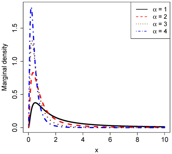
Figure 2.
The marginal densities for varied , holding and fixed.
Figure 3 plots the marginal densities for varied , holding and fixed. From the figure, we can also see that as increases, the peak value of the curve increases and the position of the peak is gradually close to zero. The marginal densities are also right-skewed.
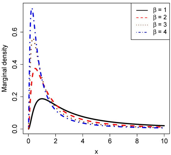
Figure 3.
The marginal densities for varied , holding and fixed.
Figure 4 plots the marginal densities for varied , holding and fixed. It is observed from the figure that as increases, the peak value of the curve decreases, and the position of the peak is gradually away from zero. Moreover, all the marginal densities are right-skewed.
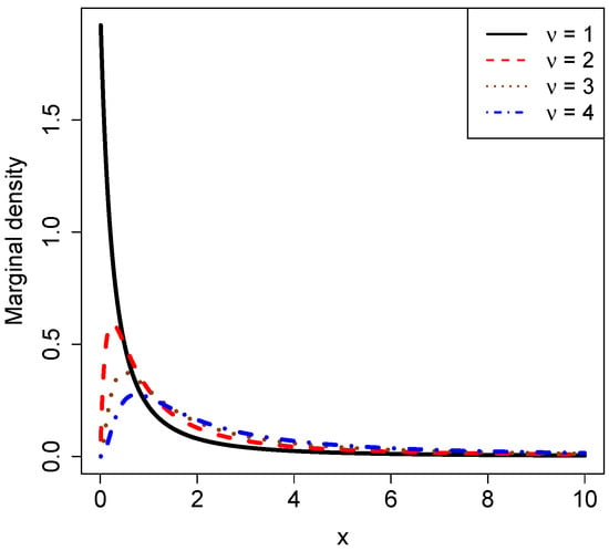
Figure 4.
The marginal densities for varied , holding and fixed.
3.2. Random Variable Generations from the Marginal Density by Three Methods
In this subsection, we generate random variables from the marginal densities by three methods. The goal of this subsection is to illustrate the theoretical result that the random variables can be generated from by three methods.
Let , , , and . Figure 5 shows the histograms of the samples generated from by the three methods:
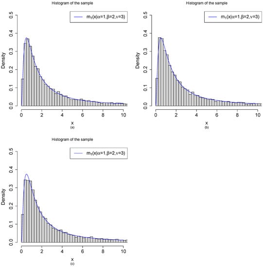
Figure 5.
Random variable generations from by three methods with , , and . (a) are iid from . (b) are iid from . (c) , where are iid from for .
- (a)
- Method 1: are generated from the model. First, we draw iid from . After that, we draw independently from .
- (b)
- Method 2: are generated from the model. First, we draw iid from . After that, we draw independently from .
- (c)
- Method 3: are generated from the transformations of beta random variables. First, we draw iid from . After that, are obtained by the transformations .
Let , , , and n = 10,000. Figure 6 shows the histograms of the samples generated from by the three methods:
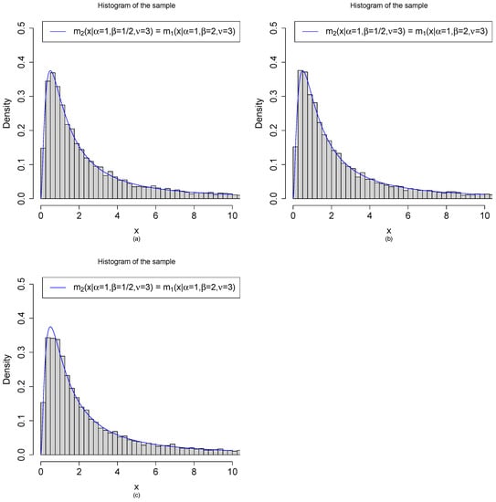
Figure 6.
Random variable generations from by three methods with , , and . (a) are iid from . (b) are iid from . (c) , where are iid from for .
- (a)
- Method 1: are generated from the model. First, we draw iid from . After that, we draw independently from .
- (b)
- Method 2: are generated from the model. First, we draw iid from . After that, we draw independently from .
- (c)
- Method 3: are generated from the transformations of beta random variables. First, we draw iid from . After that, are obtained by the transformations .
Let , , , and . Figure 7 shows the histograms of the samples generated from by the three methods:
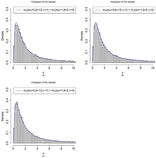
Figure 7.
Random variable generations from by three methods with , , and . (a) are iid from . (b) are iid from . (c) , where are iid from for .
- (a)
- Method 1: are generated from the model. First, we draw iid from . After that, we draw independently from .
- (b)
- Method 2: are generated from the model. First, we draw iid from . After that, we draw independently from .
- (c)
- Method 3: are generated from the transformations of beta random variables. First, we draw iid from . After that, are obtained by the transformations .
Let , , , and . Figure 8 shows the histograms of the samples generated from by the three methods:
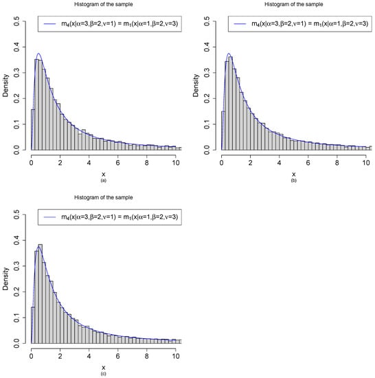
Figure 8.
Random variable generations from by three methods with , , and . (a) are iid from . (b) are iid from . (c) , where are iid from for .
- (a)
- Method 1: are generated from the model. First, we draw iid from . After that, we draw independently from .
- (b)
- Method 2: are generated from the model. First, we draw iid from . After that, we draw independently from .
- (c)
- Method 3: are generated from the transformations of beta random variables. First, we draw iid from . After that, are obtained by the transformations .
3.3. Transformations of the Moment Estimators of the Hyperparameters of One of the Eight Hierarchical Models That Have Conjugate Priors
In this subsection, we illustrate that the transformations of the moment estimators of the hyperparameters of one of the 8 hierarchical models that have conjugate priors can be used to obtain the moment estimators of the hyperparameters of another one of the 8 hierarchical models that have conjugate priors. For example, the transformations of the moment estimators of the hyperparameters of the model can be used to obtain the moment estimators of the hyperparameters of the other seven hierarchical models that have conjugate priors (, , , , , , and ). The goal of this subsection is to illustrate (3).
Let us illustrate the derivations of the moment estimators of the hyperparameters by Model 5 (). The first three moments of X are, respectively, given by
and
which can be obtained by iterated expectation. The moment estimators of , , and are calculated by equating the population moments to the sample moments, that is,
where , , is the sample kth moment of X. After some tedious calculations, we obtain
The calculations of the moment estimators of the hyperparameters of the eight hierarchical models that have conjugate priors can be found in the Supplementary Materials.
Let , , , and . The reason why we chose these values is that , , and are required in the moment estimations of the hyperparameters. Other numerical values of the hyperparameters can also be specified.
First, let us generate a random sample from the model. The histogram of the sample with the marginal density is plotted in Figure 9. From the figure, we see that the histogram fits the marginal density very well.
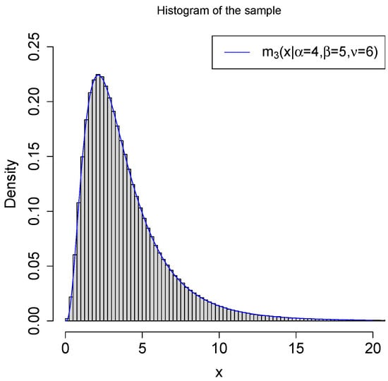
Figure 9.
The histogram of the sample with the marginal density .
Second, let us compute the moment estimators of the hyperparameters of the eight hierarchical models that have conjugate priors from the sample , and the numerical results are summarized in Table 2. Moreover, the transformations (3) of the moment estimators of the hyperparameters of the model are also summarized in this table. More precisely, for Model 5 () and Model 7 (), the identical transformation was used (, , and are unchanged); for Model 2 () and Model 4 (), the transformation was the position change of and (); for Model 6 () and Model 8 (), the transformation was replacing by (); for Model 1 () and Model 3 (), the transformation was both the position change of and and replacing by (, ). From the table, we see that the moment estimators of the hyperparameters of the eight hierarchical models that have conjugate priors and the transformations of the moment estimators of the hyperparameters of the model are the same.

Table 2.
The moment estimators of the hyperparameters of the 8 hierarchical models that have conjugate priors and the transformations of the moment estimators of the hyperparameters of the model.
3.4. The Marginal Densities of the Eight Hierarchical Models That Do Not Have Conjugate Priors
In this subsection, we obtain some conclusions about the properties of the eight marginal densities that do not have a closed form by simulation techniques and numerical integration. We take the hierarchical model as an example. The results for the other seven hierarchical models that do not have conjugate priors are similar, and thus, they are omitted. The results thus obtained are compatible with those in Section 2.2. The goal of this subsection is to obtain some conclusions about the properties of the eight marginal densities that do not have a closed form.
The histogram of the sample with sample size from the hierarchical model with , , and and the fit marginal densities are plotted in Figure 10. In Plot (a), the histogram is fit by ,. From this plot, we see that the histogram is poorly fit by the marginal densities. In other words, the four marginal densities ,, are not the marginal densities for the hierarchical model with , , and . In Plot (b), the histogram is fit by the four marginal densities ,, where , , and are the moment estimators of the hyperparameters. Moreover, the histogram is also fit by given by (1). From this plot, we see that the four marginal densities , , are the same, as the four curves overlap. It is easy to see that the four marginal densities do not fit the histogram well, especially when x is close to 0. It is worth noting that the marginal density fits the histogram very well. We would like to point out that the marginal density given by (1) was numerically evaluated by an R built-in function integrate().
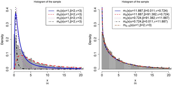
Figure 10.
The histogram of the sample with sample size from the hierarchical model with , , and and the fit marginal densities. (a) The histogram is fit by ,. (b) The histogram is fit by ,, where , , and are the moment estimators of the hyperparameters. Moreover, the histogram is also fit by .
The fit marginal densities, D-values, and p-values of the one-sample Kolmogorov–Smirnov (KS) test for a sample with sample size from the hierarchical model when , , and are summarized in Table 3. In this table, it is worth noting that the D-values and p-values of the four marginal densities ,, are the same, where , , and are the moment estimators of the hyperparameters. From the table, we see that the p-values for the first eight marginal densities are all less than , which indicates that the sample is not from the first eight marginal densities. However, the p-value for the marginal density is , which indicates that the sample can be regarded as generated from the marginal density . Moreover, the D-value for the marginal density is , which is the smallest among the D-values in this table. Therefore, the marginal density of the hierarchical model when , , and , , is not from the family of marginal densities (4). It is worth pointing out that the argument stop.on.error = FALSE is needed in integrate() to avoid the error that the “roundoff error is detected in the extrapolation table” when x is a small value, less than, say, , when applying the one-sample KS test for .

Table 3.
The fit marginal densities, D-values, and p-values of the one-sample KS test for a sample with sample size from the hierarchical model when , , and .
4. A Real Data Example
In this section, we illustrate our method by a real data example.
The data were the close prices of the Shanghai, Shenzhen, and Beijing (SSB) A shares on 6 May 2022. The official name of the A shares is Renminbi (RMB) ordinary shares, that is shares issued by Chinese-registered companies, listed in China, and marked with a face value in RMB for trading and subscription in RMB by individuals and institutions in China (excluding Hong Kong, Macao, and Taiwan). There are 4593 SSB A shares in total; however, 18 of them did not have close prices on that day because of the suspension of trading. Therefore, the sample size of the real data (henceforth, the original data ) was 4575 . The range of the original data was , meaning the lowest close price was RMB and the highest close price was RMB . Some basic statistical indicators of the original data are summarized in Table 4. From this table, we see that the original data are right-skewed (skewness = ) and fat-tailed (kurtosis = ).

Table 4.
Some basic statistical indicators of the original data .
Moreover, the histogram of the original data with a fit marginal density is plotted in Figure 11. From the figure, we see that the marginal density does not fit the original data well. Furthermore, the one-sample KS test shows that the D-value is and the p-value (<2.2 ) is less than , indicating a bad fit of the original data by the marginal density.
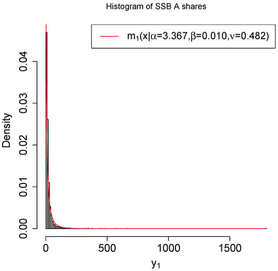
Figure 11.
The histogram of the original data with a fit marginal density .
Since the marginal density with the hyperparameters estimated by the moment estimators from the original data does not fit the original data well, we would like to transform the original data to see whether the marginal density with the hyperparameters estimated by the moment estimators from the transformed data fits the transformed data well.
In the following, we encounter some vector operations, which are defined componentwise. For example, let and be two vectors of the same length and c be a constant. Then,
Because in the marginal density , our ideas for all the transformations that will be used here are to ensure that the transformed data . A modified transformation is
where is the minimum of , , adding 1 ensures that , and the range of is . The moment estimators of the hyperparameters are , , and . Moreover, the one-sample KS test shows that the D-value is and the p-value (<2.2 ) is less than , still indicating a bad fit of the transformed data by the marginal density .
Next, we proceed with a reciprocal transformation:
where the range of is and . The moment estimators of the hyperparameters are , , and . Because the moment estimators of and are negative, the one-sample KS test cannot be performed. Hence, the marginal density cannot be used to fit the transformed data .
Similarly, we use a modified reciprocal transformation:
so that , where , and the range of is . The moment estimators of the hyperparameters are , , and . Because the moment estimators of and are negative, the one-sample KS test cannot be performed. Hence, the marginal density cannot be used to fit the transformed data .
After that, we continue with a log transformation:
where the range of is and . The moment estimators of the hyperparameters are , , and . Because the moment estimators of and are negative, the one-sample KS test cannot be performed. Hence, the marginal density cannot be used to fit the transformed data .
Similarly, we carry on with a modified log transformation:
so that , where , and the range of is . The moment estimators of the hyperparameters are , , and . Because the moment estimators of and are negative, the one-sample KS test cannot be performed. Hence, the marginal density cannot be used to fit the transformed data .
Then, we attempt a square root transformation:
where the range of is and . The moment estimators of the hyperparameters are , , and . Moreover, the one-sample KS test shows that the D-value is and the p-value (=0.0001452) is less than , still indicating a bad fit of the transformed data by the marginal density .
Finally, we seek out a modified square root transformation:
so that , where , and the range of is . The moment estimators of the hyperparameters are , , and . Moreover, the one-sample KS test shows that the D-value is and the p-value (=0.08825) is larger than , indicating a good fit of the transformed data by the marginal density .
The transformations, the moment estimators of the hyperparameters of the marginal density , and the D-value and p-value of the KS test are summarized in Table 5. In the table, the NA value indicates that the one-sample KS test cannot be performed due to some errors. From the table, we see that only the modified square root transformation can be statistically and significantly used to fit the transformed data by the marginal density . The transformation is
or

Table 5.
The transformations, the moment estimators of the hyperparameters of the marginal density , and the D-value and p-value of the KS test.
The histogram of the transformed data with a fit marginal density is plotted in Figure 12. From the figure, we see that the marginal density fits the transformed data very well.
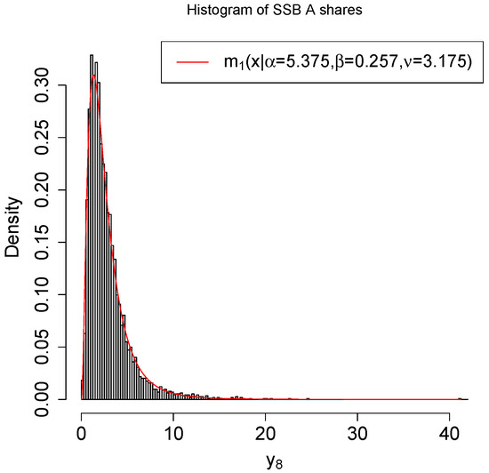
Figure 12.
The histogram of the transformed data with a fit marginal density .
5. Conclusions and Discussion
For the 16 hierarchical models of the gamma and inverse gamma distributions, there are only 8 of them that have conjugate priors, that is , , , , , , , and . We first discussed some common typical problems for the eight hierarchical models that do not have conjugate priors. Then, we calculated the Bayesian posterior densities and marginal densities of the eight hierarchical models that have conjugate priors. After that, we discussed the relations among the eight analytical marginal densities of the hierarchical models that have conjugate priors and found that there is only one family of marginal densities. Furthermore, we found some relations (6) among the random variables of the marginal densities and the beta densities. Moreover, we discussed the random variable generations for the gamma and inverse gamma distributions , , , and by using the R software.
In the numerical simulations, we plotted the marginal densities given by (2) for various hyperparameters , , and . Moreover, we illustrated the theoretical result that the random variables can be generated from by three methods from the almost identical histograms of the samples. Furthermore, we illustrated that the transformations of the moment estimators of the hyperparameters of one of the 8 hierarchical models that have conjugate priors can be used to obtain the moment estimators of the hyperparameters of another one of the 8 hierarchical models that have conjugate priors. In addition, we obtained some conclusions about the properties of the eight marginal densities that do not have a closed form by simulation techniques and numerical integration, taking the hierarchical model as an example.
We illustrated our method by a real data example, in which the original and transformed data, the close prices of the SSB A shares, were fit by the marginal density with different hyperparameters. Because in the marginal density , our ideas for all the transformations that were used were to ensure that the transformed data , .
We emphasize that the 8 hierarchical models that have conjugate priors are suitable for the study of positive, continuous, and right-skewed data, as the marginal densities of the 8 hierarchical models are positive, continuous, and right-skewed distributions. Moreover, the KS test can be used to judge whether the positive, continuous, and right-skewed data have a good fit by the marginal densities.
The eight hierarchical models that have conjugate priors are of particular interest in empirical Bayes analysis, which relies on conjugate prior modeling, where the hyperparameters are estimated from the observations by the marginal densities and the estimated prior is then used as a regular prior in the subsequent inference. See [40,48,49,50] and the references therein.
Supplementary Materials
The following Supporting Information can be downloaded at: https://www.mdpi.com/article/10.3390/math10214005/s1, Supplementary: Some proofs of the article. R folder: R codes used in the article. The R folder will be supplied after acceptance of the article.
Author Contributions
Conceptualization, Y.-Y.Z.; funding acquisition, Y.-Y.Z.; investigation, L.Z. and Y.-Y.Z.; methodology, L.Z. and Y.-Y.Z.; software, L.Z. and Y.-Y.Z.; validation, L.Z. and Y.-Y.Z.; writing—original draft preparation, L.Z. and Y.-Y.Z.; writing—review and editing, L.Z. and Y.-Y.Z. All authors have read and agreed to the current version of the manuscript.
Funding
The research was supported by the National Social Science Fund of China (21XTJ001).
Institutional Review Board Statement
Not applicable.
Informed Consent Statement
Not applicable.
Data Availability Statement
The datasets are available from the corresponding author upon reasonable request.
Conflicts of Interest
The authors declare no conflict of interest.
References
- Casella, G.; Berger, R.L. Statistical Inference, 2nd ed.; Pacific Grove: Duxbury, MA, USA, 2002. [Google Scholar]
- Shumway, R.; Gurland, J. Fitting the poisson binomial distribution. Biometrics 1960, 16, 522–533. [Google Scholar] [CrossRef]
- Chen, L.H.Y. Convergence of poisson binomial to poisson distributions. Ann. Probab. 1974, 2, 178–180. [Google Scholar] [CrossRef]
- Ehm, W. Binomial approximation to the poisson binomial distribution. Stat. Probab. Lett. 1991, 11, 7–16. [Google Scholar] [CrossRef]
- Daskalakis, C.; Diakonikolas, I.; Servedio, R.A. Learning Poisson Binomial Distributions. Algorithmica 2015, 72, 316–357. [Google Scholar] [CrossRef]
- Duembgen, L.; Wellner, J.A. The density ratio of Poisson binomial versus Poisson distributions. Stat. Probab. Lett. 2020, 165, 1–7. [Google Scholar] [CrossRef]
- Geoffroy, P.; Weerakkody, G. A Poisson-Gamma model for two-stage cluster sampling data. J. Stat. Comput. Simul. 2001, 68, 161–172. [Google Scholar] [CrossRef]
- Vijayaraghavan, R.; Rajagopal, K.; Loganathan, A. A procedure for selection of a gamma-Poisson single sampling plan by attributes. J. Appl. Stat. 2008, 35, 149–160. [Google Scholar] [CrossRef]
- Wang, J.P. Estimating species richness by a Poisson-compound gamma model. Biometrika 2010, 97, 727–740. [Google Scholar] [CrossRef] [PubMed]
- Jakimauskas, G.; Sakalauskas, L. Note on the singularity of the Poisson-gamma model. Stat. Probab. Lett. 2016, 114, 86–92. [Google Scholar] [CrossRef]
- Zhang, Y.Y.; Wang, Z.Y.; Duan, Z.M.; Mi, W. The empirical Bayes estimators of the parameter of the Poisson distribution with a conjugate gamma prior under Stein’s loss function. J. Stat. Comput. Simul. 2019, 89, 3061–3074. [Google Scholar] [CrossRef]
- Schmidt, M.; Schwabe, R. Optimal designs for Poisson count data with Gamma block effects. J. Stat. Plan. Inference 2020, 204, 128–140. [Google Scholar] [CrossRef]
- Cabras, S. A Bayesian-deep learning model for estimating COVID-19 evolution in Spain. Mathematics 2021, 9, 2921. [Google Scholar] [CrossRef]
- Wu, S.J. Poisson-Gamma mixture processes and applications to premium calculation. Commun. Stat.-Theory Methods 2022, 51, 5913–5936. [Google Scholar] [CrossRef]
- Singh, S.K.; Singh, U.; Sharma, V.K. Expected total test time and Bayesian estimation for generalized Lindley distribution under progressively Type-II censored sample where removals follow the beta-binomial probability law. Appl. Math. Comput. 2013, 222, 402–419. [Google Scholar] [CrossRef]
- Zhang, Y.Y.; Zhou, M.Q.; Xie, Y.H.; Song, W.H. The Bayes rule of the parameter in (0,1) under the power-log loss function with an application to the beta-binomial model. J. Stat. Comput. Simul. 2017, 87, 2724–2737. [Google Scholar] [CrossRef]
- Luo, R.; Paul, S. Estimation for zero-inflated beta-binomial regression model with missing response data. Stat. Med. 2018, 37, 3789–3813. [Google Scholar] [CrossRef]
- Zhang, Y.Y.; Xie, Y.H.; Song, W.H.; Zhou, M.Q. Three strings of inequalities among six Bayes estimators. Commun. Stat.-Theory Methods 2018, 47, 1953–1961. [Google Scholar] [CrossRef]
- Zhang, Y.Y.; Xie, Y.H.; Song, W.H.; Zhou, M.Q. The Bayes rule of the parameter in (0,1) under Zhang’s loss function with an application to the beta-binomial model. Commun. Stat.-Theory Methods 2020, 49, 1904–1920. [Google Scholar] [CrossRef]
- Gerstenkorn, T. A compound of the generalized negative binomial distribution with the generalized beta distribution. Cent. Eur. J. Math. 2004, 2, 527–537. [Google Scholar] [CrossRef]
- Broderick, T.; Mackey, L.; Paisley, J.; Jordan, M.I. Combinatorial clustering and the beta negative binomial process. IEEE Trans. Pattern Anal. Mach. Intell. 2015, 37, 290–306. [Google Scholar] [CrossRef] [PubMed]
- Oliveira, C.C.F.; Cristino, C.T.; Lima, P.F. Unimodal behaviour of the negative binomial beta distribution. Sigmae 2015, 4, 1–5. [Google Scholar]
- Heaukulani, C.; Roy, D.M. The combinatorial structure of beta negative binomial processes. Bernoulli 2016, 22, 2301–2324. [Google Scholar] [CrossRef]
- Zhou, M.Q.; Zhang, Y.Y.; Sun, Y.; Sun, J.; Rong, T.Z.; Li, M.M. The empirical Bayes estimators of the probability parameter of the beta-negative binomial model under Zhang’s loss function. Chin. J. Appl. Probab. Stat. 2021, 37, 478–494. [Google Scholar]
- Jiang, C.J.; Cockerham, C.C. Use of the multinomial dirichlet model for analysis of subdivided genetic populations. Genetics 1987, 115, 363–366. [Google Scholar] [CrossRef] [PubMed]
- Lenk, P.J. Hierarchical bayes forecasts of multinomial dirichlet data applied to coupon redemptions. J. Forecast. 1992, 11, 603–619. [Google Scholar] [CrossRef]
- Duncan, K.A.; Wilson, J.L. A Multinomial-Dirichlet Model for Analysis of Competing Hypotheses. Risk Anal. 2008, 28, 1699–1709. [Google Scholar] [CrossRef] [PubMed]
- Samb, R.; Khadraoui, K.; Belleau, P.; Deschenes, A.; Lakhal-Chaieb, L.; Droit, A. Using informative Multinomial-Dirichlet prior in a t-mixture with reversible jump estimation of nucleosome positions for genome-wide profiling. Stat. Appl. Genet. Mol. Biol. 2015, 14, 517–532. [Google Scholar] [CrossRef] [PubMed]
- Grover, G.; Deo, V. Application of Parametric Survival Model and Multinomial-Dirichlet Bayesian Model within a Multi-state Setup for Cost-Effectiveness Analysis of Two Alternative Chemotherapies for Patients with Chronic Lymphocytic Leukaemia. Stat. Appl. 2020, 18, 35–53. [Google Scholar]
- Mao, S.S.; Tang, Y.C. Bayesian Statistics, 2nd ed.; China Statistics Press: Beijing, China, 2012. [Google Scholar]
- Zhang, Y.Y.; Ting, N. Bayesian sample size determination for a phase III clinical trial with diluted treatment effect. J. Biopharm. Stat. 2018, 28, 1119–1142. [Google Scholar] [CrossRef] [PubMed]
- Zhang, Y.Y.; Ting, N. Sample size considerations for a phase III clinical trial with diluted treatment effect. Stat. Biopharm. Res. 2020, 12, 311–321. [Google Scholar] [CrossRef]
- Zhang, Y.Y.; Rong, T.Z.; Li, M.M. The estimated and theoretical assurances and the probabilities of launching a phase iii trial. Chin. J. Appl. Probab. Stat. 2022, 38, 53–70. [Google Scholar]
- Zhang, Y.Y.; Ting, N. Can the concept be proven? Stat. Biosci. 2021, 13, 160–177. [Google Scholar] [CrossRef]
- Robert, C.P. The Bayesian Choice: From Decision-Theoretic Motivations to Computational Implementation, 2nd ed.; Springer: New York, NY, USA, 2007. [Google Scholar]
- Zhang, Y.Y. The Bayes rule of the variance parameter of the hierarchical normal and inverse gamma model under Stein’s loss. Commun. Stat.-Theory Methods 2017, 46, 7125–7133. [Google Scholar] [CrossRef]
- Chen, M.H. Bayesian Statistics Lecture; Statistics Graduate Summer School, School of Mathematics and Statistics, Northeast Normal University: Changchun, China, 2014. [Google Scholar]
- Xie, Y.H.; Song, W.H.; Zhou, M.Q.; Zhang, Y.Y. The Bayes posterior estimator of the variance parameter of the normal distribution with a normal-inverse-gamma prior under Stein’s loss. Chin. J. Appl. Probab. Stat. 2018, 34, 551–564. [Google Scholar]
- Zhang, Y.Y.; Rong, T.Z.; Li, M.M. The empirical Bayes estimators of the mean and variance parameters of the normal distribution with a conjugate normal-inverse-gamma prior by the moment method and the MLE method. Commun. Stat.-Theory Methods 2019, 48, 2286–2304. [Google Scholar] [CrossRef]
- Sun, J.; Zhang, Y.Y.; Sun, Y. The empirical Bayes estimators of the rate parameter of the inverse gamma distribution with a conjugate inverse gamma prior under Stein’s loss function. J. Stat. Comput. Simul. 2021, 91, 1504–1523. [Google Scholar] [CrossRef]
- Lee, M.; Gross, A. Lifetime distributions under unknown environment. J. Stat. Plan. Inference 1991, 29, 137–143. [Google Scholar]
- Pham, T.; Almhana, J. The generalized gamma distribution: Its hazard rate and strength model. IEEE Trans. Reliab. 1995, 44, 392–397. [Google Scholar] [CrossRef]
- Agarwal, S.K.; Kalla, S.L. A generalized gamma distribution and its application in reliability. Commun. Stat.-Theory Methods 1996, 25, 201–210. [Google Scholar] [CrossRef]
- Agarwal, S.K.; Al-Saleh, J.A. Generalized gamma type distribution and its hazard rate function. Commun. Stat.-Theory Methods 2001, 30, 309–318. [Google Scholar] [CrossRef]
- Kobayashi, K. On generalized gamma functions occurring in diffraction theory. J. Phys. Soc. Jpn. 1991, 60, 1501–1512. [Google Scholar] [CrossRef]
- Al-Saleh, J.A.; Agarwal, S.K. Finite mixture of certain distributions. Commun. Stat.-Theory Methods 2002, 31, 2123–2137. [Google Scholar] [CrossRef]
- R Core Team. R: A Language and Environment for Statistical Computing; R Foundation for Statistical Computing: Vienna, Austria, 2022. [Google Scholar]
- Berger, J.O. Statistical Decision Theory and Bayesian Analysis, 2nd ed.; Springer: New York, NY, USA, 1985. [Google Scholar]
- Maritz, J.S.; Lwin, T. Empirical Bayes Methods, 2nd ed.; Chapman & Hall: London, UK, 1989. [Google Scholar]
- Carlin, B.P.; Louis, A. Bayes and Empirical Bayes Methods for Data Analysis, 2nd ed.; Chapman & Hall: London, UK, 2000. [Google Scholar]
Publisher’s Note: MDPI stays neutral with regard to jurisdictional claims in published maps and institutional affiliations. |
© 2022 by the authors. Licensee MDPI, Basel, Switzerland. This article is an open access article distributed under the terms and conditions of the Creative Commons Attribution (CC BY) license (https://creativecommons.org/licenses/by/4.0/).