Abstract
This paper explores two Omnichannel retail models consisted of one online platform and one brick-and-mortar store under different power structures considering cost-sharing mechanisms. In retail supply chain dominated by the online platform and brick-and-mortar store, respectively, under a “Buy online and pick up in store” strategy, the influences of the cost-sharing ratio and the proportion of traditional consumers on pricing and service decisions, the demands of various groups of consumers, and the performance of the retail system have been examined. In addition, the results of decision-making and profitabilities of retailers under different power structures have also been considered. The key findings show that the optimal price and service level first increase and then decrease with the cost-sharing ratio in a retail system dominated by the online platform. In contrast, the price and service level increase with the cost-sharing ratio only when the proportion of traditional consumers is relatively large in a retail system dominated by brick-and-mortar store. The symmetry demand increases as the scale of traditional consumers shrinks when the cost-sharing ratio is relatively large in a retail system dominated by the online system. At the same time, it only increases when the cost-sharing ratio is in the range of in a retail system dominated by the brick-and-mortar store. No matter what the power structure is, the profit of the retail system always first increases and then decreases with the proportion of traditional consumers. Additionally, when the cost-sharing ratio and the proportion of traditional consumers are relatively small, the total demand in the retail system dominated by the online platform is higher than that in the retail system dominated by the brick-and-mortar store. The total profit is larger in the online platform-dominated retail system than that in the brick-and-mortar store-dominated retail system when the cost-sharing ratio is relatively high. However, when the cost-sharing ratio is relatively low, the profitability of the brick-and-mortar store-dominated retail system is stronger.
Keywords:
omnichannel retailing; power structure; cost-sharing mechanism; consumer composition; buy online and pick-up in store MSC:
90B06
1. Introduction
The rapid development of e-commerce and the increasing maturity of mobile payments have not only given rise to many new retail models but also profoundly influenced the consumers’ shopping habits and preferences. The upgrading of consumption quality has prompted consumers to pay more attention to the timeliness and convenience of shopping, thus further promoting the integration of online and offline sales channels. Traditional retail giants represented by Walmart and Kroger, are facing the huge impact of e-commerce development. They are continuously reducing their offline stores while focusing on the layout of online channels. Based on the increasing personalized needs of consumers, the e-commerce platforms represented by Amazon are actively expanding offline channels while increasing customer stickiness through price concession strategies (Jindal et al., 2021 [1]). In the process of exploring the development of channel integration, omnichannel retail models such as Showrooms, HTO (Home Try-on), STS (Ship To Store), and BOPS (Buy Online and Pick up in Store) have come into being. Uncertain risk factors such as the COVID-19 epidemic have also prompted new omnichannel retail formats such as community group buying to become hot spots of public attention. Compared with traditional retail models, omnichannel retail aims to provide seamless, consistent and more reliable services for consumers by coordinating processes and technologies across all channels (Verhoef et al., 2015 [2]). According to the four stages of the value-adding journey of consumers, the channel integration process unfolds based on four main stages that are pre-purchase, payment, delivery, and return (Saghiri et al., 2017 [3]), thus forming a full-flow, convenient shopping and feedback system. Among the existing omnichannel retail models, the BOPS (Buy Online and Pick up in Store) model is the most important omnichannel initiative that promotes the integration of online and offline (Li et al., 2020 [4]), providing a continuous, complete, and seamless shopping experience for consumers and widely used in the domestic and international retail industry. Retail giants such as Macy’s and Uniqlo have been exploring and implementing the BOPS model, which not only realizes the digital participation of offline consumers but also greatly broadens the breadth of products available for sale in offline stores. The huge advantages of online and offline integration provide new growth points for the development of the retail industry and point out new directions for the innovative transformation of retail modes.
The BOPS omnichannel retail model provides consumers with a seamless and complete shopping experience based on the integration of online and offline channels, and puts forward higher requirements for the collaboration among the various entities in the retail system. This cooperation and integration lead to conflicts of interest among supply chain members. Furthermore, the heterogeneity of consumer channel selection and free-riding behavior exacerbates the conflicts between channel members. For example, DairaDish, a Chinese fresh food brand using the BOPS model to provide fresh food retail services to the community, fails to properly distribute store profits equitably during the rapid expansion of its offline stores, resulting in uneven service levels and inefficient integration of online and offline channels (Zhang et al., 2020 [5]). It eventually declares bankruptcy and reorganizes in 2020 due to poor operations. How to pay attention to the behavioral preferences of each channel member promptly and adopt a reasonable mechanism to coordinate the cooperation between retail entities has become an important issue that needs to be addressed to improve the efficiency of omnichannel retail operations and enhance the stability of the retail supply chain.
Motivated by the demand of coordination between retail entities and different consumer groups, this paper establishes a game model consisted of one online platform and one brick-and-mortar store, and explores the decision-making behaviors and each entity’s performances under different dominated models considering the cost-sharing mechanism. The following questions are addressed in this paper.
- (1)
- How does the cost sharing ratio impact the optimal pricing and service decisions of the supply chain members?
- (2)
- How do the consumer heterogeneity and consumer composition affect retailers’ pricing and service decisions?
- (3)
- Which model yields the best decisions of the omnichannel retail system?
- (4)
- How should the brand retailers adjust operating decisions to maximize profits under different power structures considering consumer heterogeneity?
We organize the rest of the paper as follows. The related literature is reviewed in Section 2. We depict the study context and introduce the model in Section 3. In Section 4, we derive and display the equilibrium solutions. Section 5, Section 6 and Section 7 demonstrate and analyze the conclusions derived from the equilibrium solutions. Finally, we conclude the paper in Section 8. All the proofs are presented in the Appendix A.
2. Literature Review
This article explores the operation decisions of retailers, the demand for products, and the profitability of retail subjects under different power structures, considering the cost-sharing mechanism in the BOPS omnichannel retail model. There are three closely related streams of literature, namely, BOPS omnichannel retail, cost-sharing mechanism, and power structure in supply chain.
2.1. BOPS Omnichannel Retail
The concept of Omnichannel Retail first appears in Darrell Rigby’s “The Future of Shopping” in 2011. He points out that in the omnichannel environment, retailers can integrate brick-and-mortar stores, online stores, social media, and other channels to interact with consumers. On this premise, Levy et al. (2013) [2] further interpret omnichannel retail from the consumer perspective as “a coordinated multichannel that offers a seamless experience when using all the retailers’ shopping channels.” Currently, the industry has developed various omnichannel retail models such as BOPS (Buy Online and Pick up in-store), STS (Ship to Store), HTO (Home Try-on), and Showrooms. BOPS is considered as the most important omnichannel initiative to promote the integration of online and offline channels (Li et al., 2020 [4]). It is one of the focuses of academic research at present. Research on operational decision-making based on the BOPS omnichannel retail model has yielded many achievements. The existing studies mainly focus on inventory decision and pricing decision. Regarding inventory decision, Gallino et al. (2017) [6] and Gao et al. (2017) [7] explore the inventory decisions considering the coordination between online and offline demands by empirical research method and modeling research method, respectively. Lu et al. (2020) [8] analyze the optimal decisions of product order-quantity and inventory-allocation for meeting both store and BOPS demands. From the pricing decision perspective, Jiang et al. (2020) [9] analyze the optimal pricing decisions under the BOPS retail model considering service level. Liu et al. (2020) [10] explore the joint decision on pricing and ordering for BOPS retailers, and find the optimal decisions are related to the percentage of consumers preferring each channel. Li et al. (2021) [11] examine the pricing decisions and profits in the omnichannel retail system considering coupon value and service effort. It is worth noting that the above literature is set in models with specified dominants, such as an online platform or a brick-and-mortar store. In contrast to the above research, our study also considers the impact of different dominated models on pricing decisions.
The expansion of retail channels under the BOPS model not only affects retailers’ pricing decisions, but also leads to the differentiation of consumer groups in terms of channel choice. Existing studies have shown that consumer heterogeneity is a potentially important driver of omnichannel convergence (Shen et al.,2018 [12]), and different consumer channel preferences affect the channel operation decisions. Therefore, the heterogeneity of consumer channel choice has become the scholars’ focus. Existing studies show that studies centering on customer segmentation are strongly related to different consumers’ choice drivers and behaviors across channels (Pauwels et al., 2015 [13]; Wang et al., 2015 [14]). For example, Hsiao et al. (2014) [15] and Zhang et al. (2017) [16] classify consumers into grocery shoppers and priori Internet shoppers to investigate. Hu et al. (2022) [17] divide consumers into two segments, namely store-only customers and omni-customers. Jin et al. (2018) [18] argue that online consumers in the BOPS model are deterministic while off-line consumers are discretionary, and study the service area design of retailers under this assumption. Liu et al. (2020) [9] find the joint decisions on pricing and ordering for BOPS retailers are related to the proportion of online channel buyers and store channel buyers. Therefore, based on the above literature, our study classifies consumers according to their heterogeneity considering the characteristics of BOPS omnichannel retail.
2.2. Cost-Sharing Mechanism
With the expansion of product channels and the improvement of industrial operation efficiency, the collaboration between supply chain members is becoming closer and closer. In order to enhance channel partnership and improve the operational efficiency of the supply chain, cost-sharing has become an important strategy of widespread concern in the industrial and academic communities. The design and implementation of the cost-sharing mechanism can improve the supply chain system’s operational decision efficiency and strongly influence each supply chain entity’s strategy choice and profitability. There are many studies related to the cost-sharing mechanism based on the traditional two-echelon supply chain. Zhou et al. (2018) [19] explore the cost-sharing mechanism in a two-echelon supply chain where a manufacturer sells products through both her own online channel and a traditional retailer. Chakraborty et al. (2018) [20] introduce cost-sharing contracts in retailer-led quality innovation collaborations to promote supply chain members and overall profitability. Fan et al. (2020) [21] consider a two-echelon supply chain in which an upstream manufacturer and a downstream retailer share the product liability cost caused by quality defects. Apart from traditional retail supply chain models, although Chen et al. (2021) [22] consider advertising cost sharing and consumer migration in an omnichannel retail model, the impacts of cost-sharing ratios on the operation decisions and profitability of retailer need to be further explored. In contrast to the above research, we focus on the impacts cost-sharing ratios on omnichannel retail decisions under different power structures.
2.3. Power Structure
Channel power refers to the control and influence of one channel member over the operational decision variables of channel members at different distribution levels (Schul, 1983 [23]). The dominant player in the supply chain with channel power has the first-moving advantage in decision making and can influence the decision-making behaviors of other supply chain participants (followers) by prioritizing the order of decisions. Luo et al. (2018) [24] explore the impact of power structure and find it has a great influence on supply chain members’ pricing policies and performances. Li et al. (2019) [25] explore the power structure in a dual-channel supply chain consisted of a manufacturer and a retailer providing services. They find that in the presence of the showroom effect, a later decision sequence for the retailer is beneficial to the profitability of the retailer and the supply chain. Yan et al. (2020) [26] study price competition between the e-commerce platform and the supplier in a dual-channel supply chain. This research concluds that the e-platform gains a first-mover advantage by announcing its prices earlier in the supply chain. Matsui (2021) [27] explore how the power structure influences supply chain members’ profitabilities in a three-echelon supply chain facing chiastic demand.
It is worth noting that the above studies on the power structure in the retail supply chain are based on two subjects that are the manufacturer and retailer. However, in the retailer’s BOPS omnichannel retail model, the entire retail system is consisted of only the online platform and the brick-and-mortar store, so research on the influence of power structure on omnichannel retail is limited. However, the issue of channel integration under different dominated models has gradually become an issue that cannot be ignored. This research focuses on the impact of power structure on decision-making in the BOPS retail model under the cost-sharing mechanism. Moreover, we explore the roles of cost sharing ratio and the scale of traditional consumers in retail model to provide a useful reference for the operation of BOPS omnichannel retail.
3. Problem Definitions
In this study, we investigate the impacts of different power structures, considering offline service cost allocation on the BOPS retail business model containing an online platform and a brick-and-mortar store, as well as examine their optimal pricing and service decisions in a competitive market. Figure 1 presents the market structure with the specific sales channels of the BOPS retail model that deliver the products to consumers. We consider the omnichannel retail system of a brand that distributes its products through the online platform and brick-and-mortar store, the online and offline retailers manage the two channels, respectively, and cooperate in providing “buy online and pick up in store” service. BOPS consumers pick up products and receive service in brick-and-mortar stores after placing orders online to realize the integration of the online and offline retailing channels.
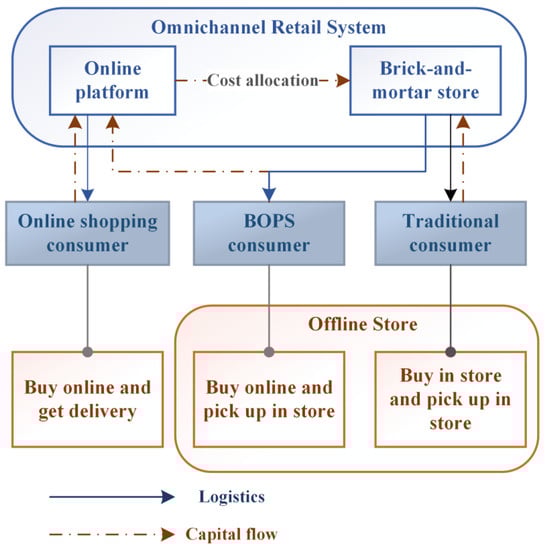
Figure 1.
BOPS omnichannel retail model.
In Figure 1, the full lines depict the physical flow in the retail system, and the dotted lines represent the information flow in the retail system. In this study scenario, the BOPS sales volume is included in the online channel since consumers reserve and pay online. At the same time, the brick-and-mortar store needs to provide service for BOPS consumers, such as a comfortable experience environment, offering trial samples, friendly front-line staff with enthusiastic service, and attractive shelf displays (Zhou et al., 2018 [19]). Thus, the online retailer is asked to undertake part of the cost of offline service to reduce channel conflict and compensate for the brick-and-mortar store’s additional efforts. Following the practices of firms such as Target, Walmart, and Zara, we assume that the retailer sets a uniform price across different channels (Balakrishnan et al., 2014 [28]; Bell et al., 2018 [29]; Li et al., 2021 [11]). Under the omnichannel retail mode, the online platform and the brick-and-mortar store determine the unified retail price and service levels, respectively. Scenario U and Scenario D are divided according to the different power structures in this Stackelberg game. In Scenario U, the online platform makes its first move and announces its selling price. Based on the online platform’s decisions, the following brick-and-mortar store determines the level of offline service. Contrary to the above, the brick-and-mortar store first sets the service level, and the online platform determines the unified selling price afterwards in Scenario D.
In the omnichannel retail market, consumers are divided into the following three segments according to different consumption habits, and this classification method has been widely used in the existing literature. The first segment covers traditional consumers who only purchase products and experience service in the brick-and-mortar store. represents the proportion of traditional consumers. For simplicity, consumer’s sensitivity to the retail price and service level is normalized to 1. Following studies of Martín et al. (2015) [30], Li et al. (2019) [31], and Nie et al. (2019) [32], we employ a linear demand model to characterize the demand function. Thus, the demand function of traditional consumers is . The second segment includes BOPS consumers who purchase products online and go to the brick-and-mortar store to pick up commodities and experience services. Therefore, the service level of offline retailers has a certain influence on the demand of BOPS consumers. On the premise that represents the proportion of BOPS consumers, the demand function of BOPS consumers is . The third segment covers online shopping consumers who only buy on online platforms and require retailers to deliver directly to their homes. Hence the demand of online shopping consumers is not affected by the offline service level. The demand function of online shopping consumers is consequently. It is assumed that customers will not switch between segments for reasons other than pricing and service level. Additionally, is used to represent the level of service provided by the brick-and-mortar store. It is assumed that the cost function of service is according to Li et al. (2022) [33], which satisfies , , and . Moreover, the proportion of the online platform required to assume the cost of offline services is , which implies the service costs borne by the online platform and the brick-and-mortar store are and , respectively. As mentioned above, the symbolic description of the model and the notations are summarized in Table 1.

Table 1.
The symbolic description.
4. Model Formulation and Solution
As mentioned earlier, scenario U and scenario D are examined to model the effects of power structure on pricing and service decision. In summary, in the first scenario, the online platform owns the first-moving advantage as the Stackelberg leader to take the lead in determining the unified retail price. While in the second scenario, the leadership is mastered by the brick-and-mortar store, and the platform determines the selling price according to the service level decided by the offline store as the follower.
In Scenario U, the online platform determines the unified selling price first, and the brick-and-mortar store sets the service level afterward. Equations (1)–(3) represent the profit functions of the online platform, the brick-and-mortar store, and the retail system, respectively.
Maximizing the profit function yields each channel’s pricing and service decisions. In the Stackelberg game, the optimal decisions of online platform and brick-and-mortar store are determined through the backward induction method. Through this approach, the optimal response function of the offline retailer calculated from is . Substitute this formula into (1). The optimal unified retail price is based on the online platform’s first-order condition of profit maximization. The optimal service level can be calculated by substituting this formula into the optimal response function of the offline retailer . While in Scenario D, the offline retailer (the brick-and-mortar store) makes its first move and determines its service level. The online platform determines the uniform retail price based on the offline retailer’s strategy. By backward induction, the optimal solutions in Scenario U and Scenario D are shown in Table 2.
Table 2.
The optimal strategies for Scenario U and Scenario D.
5. BOPS Supply Chain Dominated by the Online Platform (Scenario U)
5.1. Insights on Impacts of Cost-Sharing Ratio
In order to explore the cost-sharing mechanism under the BOPS retail system dominated by the online platform, this subsection studies the impacts of the cost-sharing proportion of the online platform on price and service strategies, the demand of different groups of consumers, and the profit of each retailing entity, respectively.
Proposition 1.
In the BOPS model dominated by the online platform,
- (i)
- Priceincreases with the cost-sharing ratiowhenand then decreases when;
- (ii)
- Service levelincreases with the cost-sharing ratiowhenand then decreases when.
Proposition 1 indicates that the level of offline service and the uniform sales price increase first and then decrease with the cost-sharing ratio, and the change of service levels lags behind the change in retail price. Since the cost-sharing mechanism stimulates the brick-and-mortar store to improve service motivation and simultaneously pushes up the operational costs of the online platform. Hence the service level and uniform price have positive relationships with the proportion of cost allocation initially. However, with the increase in sales price, the demand of online shopping consumers gradually decreases, as reflected in the transfer of some consumers to other channels or even the loss of some customers. This change prompts the online platform to reduce the retail price to ensure profits. Further, the decline in uniform sales price forces the brick-and-mortar store to lessen the service level to reduce operational costs.
This conclusion also implies that the uniform retail price and offline service reach the highest level when and , respectively. In other words, there is an optimal cost allocation ratio to enable traditional and BOPS consumers to enjoy the best offline services, which requires consumers to expend higher costs.
Moreover, due to the first-moving advantage of the online platform as the leader in the Stackelberg game, the brick-and-mortar store is passive in decision making. Therefore, compared with the pricing decision of the online platform, the service decision of the brick-and-mortar lags in response to changes in cost-sharing proportion, therefore the cut-off point of service level is greater than that of the sales price . In order to visually reflect the changes in service level and retail price to the apportionment ratio, the price and service graphics are plotted in Figure 2 by setting and . Figure 2 displays that uniform and service level both increase first and then decrease with the cost ratio varying from 0 to 1, and attain their maximum values when equals 1/2 and 1/3 respectively, where the trend of lags behind the trend of .
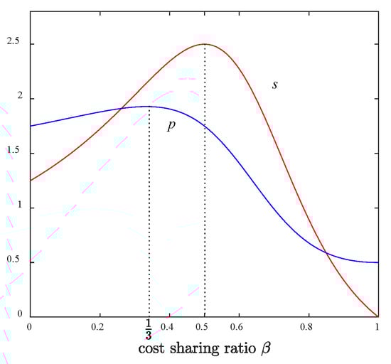
Figure 2.
Pricing and service decisions in Scenario U.
Proposition 2.
In the BOPS model dominated by the online platform,
- (i)
- The demand of traditional consumersand the demand of the BOPS consumersincrease with the cost-sharing ratiowhenand decrease when.
- (ii)
- The demand of online shopping consumersdecreases with the cost-sharing ratio when, and increases when.
- (iii)
- The total demand of the retail systemincreases with the ratiowhen, and decreases when.
Proposition 2 shows that with the increase in cost sharing proportion, the demand of online shopping consumers first decreases and then increases. In contrast, the demands of traditional consumers and BOPS consumers first increase and then decrease. Based on the sales results of various groups of consumers, the aggregate demand of the retail system amplifies first and then decreases along with the magnification of allocation proportion.
In the BOPS retail system, the demand of online shopping consumers is not influenced by the level of service accepted by traditional and BOPS consumers. In contrast, the fluctuation of uniform retail prices plays a leading role. Consequently, it fluctuates in the opposite direction of the changes in the retail price synchronously. At beginning, with the expansion of the cost allocation ratio, the online platform increases sales price along with the increasing operating costs, which leads to the reduction of online shopping demand and the transfer of consumers to other channels. Hence, the online platform reduces the sales price to ensure profits, and the demand of online shopping consumers is directly affected to increase. As for traditional and BOPS consumers, their demands are influenced by both the service level and sales price, which increase first and then decrease as the proportion of cost allocation increases. This trend reflects the stimulating effect of improving service levels in the initial stage of the cost allocation mechanism. However, it also reveals that the increasing cost burden of the online platform can also lead to the decline in the aggregate demand of the retail system. That is, the change in the total demand of the retail system with the proportion of allocation shows the shape of an inverted U, and the fixed point of the inverted U-shaped graph appears at . In other words, the retail system can obtain the maximum demand when the allocation ratio is equal to . By setting , , and , Figure 3 shows the U-shaped graph of and the inverted U-shaped graphs of , and as the cost-sharing ratio increases.
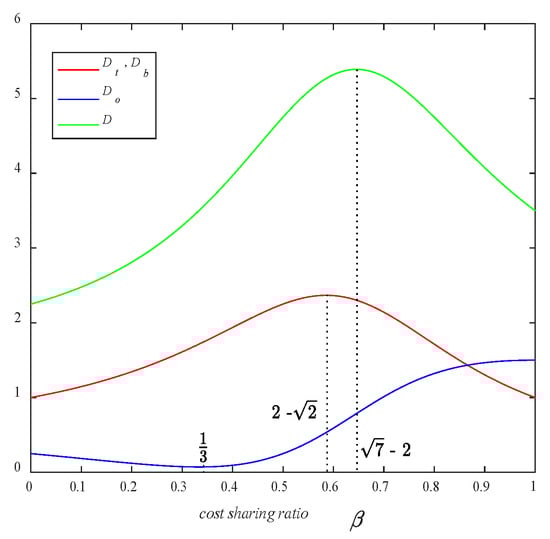
Figure 3.
Demand in Scenario U.
In addition, the relationship between every variable and the ratio of cost allocation can be shown in Table 3. It can be concluded from the table that the demand of online shopping consumers is the least when , and the demands of traditional consumers, BOPS consumers, and the aggregate demand of the retail system reach the maximum when , , respectively. In addition, for both the online platform and the brick-and-mortar store, when the cost-sharing ratio is in range of , all entities of the retail system have the enthusiasms to promoting the expansion of the cost allocation ratio undertaken by the online platform to expand demand.
Table 3.
The variation in demand with the cost-sharing ratio.
Proposition 3.
In the BOPS model dominated by the online platform,
- (i)
- The profit of the online platformincreases with the cost-sharing ratiowhen, and decreases when.
- (ii)
- The profit of the brick-and-mortar storeincreases at the threshold, and decreases at the threshold.
- (iii)
- The profit of the retail systemdecreases in the threshold, and increases in the threshold.
Additionally,
.
Proposition 3 indicates that with the increase in the cost-sharing proportion, the profits of the online platform tend to increase first and then decline, and reach the maximum when . This conclusion implies that in the initial stage, the cost allocation mechanism can promote the expansion of demand, thereby enhancing the profitability of the online platform. However, there is also an optimal allocation proportion for the online platform. If the allocation proportion exceeds the value , the profit of the online platform declines with the increase in allocation ratio due to the expansion of operating costs. Compared with the online platform, the change in brick-and-mortar store’s profit to cost allocation ratio is more complex concerning the proportion of traditional consumers. Only when the proportion of traditional consumers meets the condition does the profit of the brick-and-mortar store increase with the allocation ratio; On the contrary, the profit of the offline store declines as the sharing proportion increases. Based on the profitability of each channel, the changing trend of the aggregate profit of the retail system with the allocation ratio is as follows. When the proportion of traditional consumers meets the condition , the profit of the retail system declines as the allocation ratio increases; Conversely, the retail system’s profit increases with the increase in the cost-sharing proportion.
5.2. Insights on the Proportion of Traditional Consumers
Proposition 4.
In the BOPS model dominated by the online platform,
- (i)
- Priceand service leveldecrease with the proportion of traditional consumers.
- (ii)
- The demand of traditional consumersincreases with the proportion of traditional consumers; the demand of BOPS consumersand the demand of online shopping consumersdecrease with.
- (iii)
- The symmetry demand of the retail systemincreases with the proportion of traditional consumersunder the threshold, and decreases in the threshold.
Proposition 4 displays the trend of optimal service level, uniform sales price, and the demand of each group of consumers as the proportion of cost allocation changes. It can be concluded from the proposition that both service level and the retail price change in the opposite direction with the proportion of traditional consumers. The reason is that, with the increase in the proportion of traditional consumers, the demands for the online channel and the BOPS channel are squeezed. Thus, the online platform reduces the uniform price to ensure profits. The expansion of the scale of traditional consumers leads to the decline in the uniform retail price.
Meanwhile, the brick-and-mortar store has to cut operating costs by reducing the service level on the premise of a decline in sales price. Therefore, the service level and the uniform price decline as the proportion of traditional consumers increases. This result also implies that in the early stage of implementing the omnichannel retail model, the brick-and-mortar store constantly improves the level of offline service to reduce the loss of consumers as the proportion of traditional consumers gradually shrinks. At the same time, the increase in operating costs also promotes the increase in the uniform price of the retail system.
With the expansion of the proportion of traditional consumers, the demand for traditional consumers gradually increases, while the demands of online shopping and BOPS consumers gradually decline. Reflected in the reality of the deployment of the omnichannel retail model, in the initial stage, the shrinking scale of traditional consumers leads to the reduction of their demands, and the consumers’ behavior of channel transfer results in the increase in the demands of online shopping consumers and BOPS consumers. This conclusion indicates that implementing the omnichannel retail model is bound to adversely influence the operation of traditional offline retailers. Based on the changes in demands of all distribution channels, the aggregate demand of the retail system changes with the proportion of traditional consumers. To be specific, when the cost allocation ratio of the online platform is relatively small (), the total demand of the retail system increases with the expansion of traditional consumers. On the contrary (), the total demand of the retail system declines as the proportion of traditional consumers increases. Based on this conclusion, the retail entities can adjust the proper cost-sharing ratio to the distribution characteristic of consumer groups in omnichannel retail.
By setting , , and , three-dimensional images, such as Figure 4, Figure 5 and Figure 6 depict the optimal pricing and service decisions, the demand of each group of consumers, and the total demand in the retail system influenced by the cost-sharing ratio and the share of traditional consumers respectively to reflect the changes visually. It can be easily observed in Figure 4 that both the optimal price and service level decrease with the proportion of traditional consumers, but they increase first with the cost-sharing ratio and then decrease, which also confirm the conclusion of proposition 1. Figure 5 displays that the demands of BOPS and online shopping consumers decrease while the demand of traditional consumers increases with the proportion of traditional consumers. Additionally, the demands of traditional consumers, BOPS consumers, and whole consumers first increase and then decrease with the cost-sharing ratio, whereas the demand of online shopping consumers changes in the opposite direction, which also confirm the conclusion of proposition 2. Figure 6 illustrates that the total demand increases with the proportion of traditional consumers when the cost-sharing ratio is less than 1/3 and decreases otherwise.
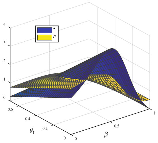
Figure 4.
Pricing and service decisions in Scenario U.

Figure 5.
Demand in Scenario U.
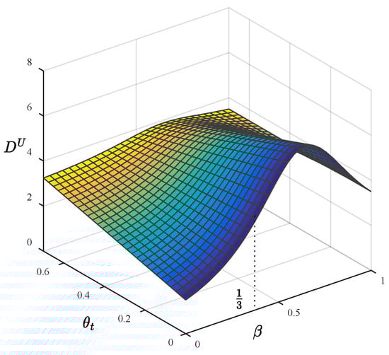
Figure 6.
Demand of the retail system in Scenario D.
The inspiration of retail enterprises is that in the initial stage of the development of omnichannel retail, the online platform should bear a relatively large proportion of service costs to obtain greater demand for the retail system as the ratio of traditional consumers shrinks, because the total demand of the retail system increases as the proportion of traditional consumers declines in that case. Conversely, if the enthusiasm of an online platform for cost allocation is relatively weak, the aggregate demand for the retail system decreases. Therefore, channel integration and cost allocation promotion strategies should be synchronous and complementary.
Proposition 5.
In the BOPS model dominated by the online platform,
- (i)
- The profit of the online platformdecreases with the proportion of traditional consumers.
- (ii)
- The profit of the brick-and-mortar storeincreases with the proportion of traditional consumerswhen, and decreasesotherwise.
- (iii)
- The profit of the retail systemincreases with the proportion of traditional consumerswhen, and decreases withotherwise.
The profits of various retail entities during the development of omnichannel retailing are shown in Proposition 5. It can be concluded that the profit of the online platform declines with the increase in the proportion of traditional consumers. The expansion of the scale of traditional consumers squeezes the demands of online shopping consumers and BOPS consumers, resulting in the decline in the online platform’s profit. Proposition 5(ii) indicates that during the deployment of omnichannel retail, the profit of the brick-and-mortar store first increases and then decreases with the reduction in the proportion of traditional consumers. In other words, there is an optimal proportion of traditional consumers to maximize the profits of the brick-and-mortar store. This result also implies that for the brick-and-mortar store, the expansion of traditional consumers is not always beneficial to obtaining profits, since the profit of the brick-and-mortar store increases as the proportion of traditional consumers declines when the ratio is relatively high. Since in the early stage of omnichannel retail development, the huge increment of demand brought by the expansion of the new channel offsets the profit loss caused by the contraction of the scale of traditional consumers. Therefore, synthesizing the profits of the online platform and the brick-and-mortar store, the gross profit of the retail system increases first and then decreases with the decline in the proportion of traditional consumers. There is an optimal proportion of traditional consumers to maximize the profit of the retail system. The change in gross profit with the proportion of traditional consumers also reveals the principle that the optimal state of omnichannel retail is the coexisting and coordinated development of multiple distribution channels, rather than squeeze the traditional channels under the background of the rapid development of e-commerce. Figure 7 depicts the changes in profits of the online platform, the brick-and-mortar store, and the retail system with the proportion of traditional consumers by setting , and . The profits of the brick-and-mortar store and the retail system show an inverted-U shape with the change IN the proportion of traditional consumers. In contrast, the expansion of the scale of traditional consumers inevitably results in a reduction in the profit of the online platform.
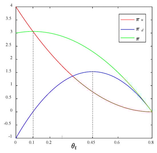
Figure 7.
Profits of entities in Scenario U.
6. BOPS Supply Chain Dominated by the Brick-and-Mortar Store (Scenario D)
6.1. Insights on Impacts of the Cost Sharing Ratio
Proposition 6.
In the BOPS model dominated by the brick-and-mortar store,
- (i)
- Priceand service leveldecrease with the cost-sharing ratio whenand increase withotherwise.
- (ii)
- The demand of traditional consumers, the demand of BOPS consumers, and the demand of the retail systemdecrease with the cost-sharing ratiowhen, and increase with otherwise. The demand of online shopping consumers increases with when , and decreases with otherwise.
Proposition 6 demonstrates the influence of online platform cost allocation proportion on pricing and service strategies and the demand of different consumers. It shows that the percentage of traditional consumers influences the trend of each variable with the cost-sharing ratio. In order to visualize and verify the above conclusions, Figure 8, Figure 9, Figure 10 and Figure 11 show trends of the variables through three-dimensional images by setting , and . It can be included that when the proportion of traditional consumers is relatively small (), the uniform retail price and service level change in the opposite direction with the cost allocation ratio as shown in Figure 8. In contrast, when the scale of traditional consumers is relatively large (), the uniform price and the level of service change in the same direction with the cost-sharing ratio as shown in Figure 9. In the actual operation process, the proportion of traditional consumers gradually shrinks in the initial promotion process of omnichannel retail. The cost allocation mechanism stimulates the service enthusiasm of the brick-and-mortar store and pushes up the operation cost. Therefore, the level of service and uniform retail price rise with the increase in cost-sharing proportion. While the proportion of traditional consumers shrinks to a certain value or even smaller, the service level and uniform retail price decrease as the ratio of cost allocation increases. This conclusion also implies that in the retail system dominated by the brick-and-mortar store, when the demand for traditional distribution channels is greatly squeezed, the cost allocation mechanism cannot stimulate the enthusiasm of the offline store to improving the quality of service.
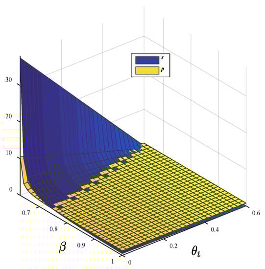
Figure 8.
Price and service in Scenario D (1).
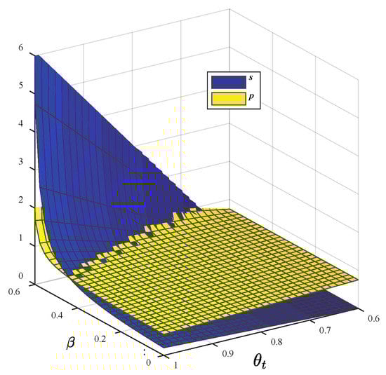
Figure 9.
Price and service in Scenario D (2).
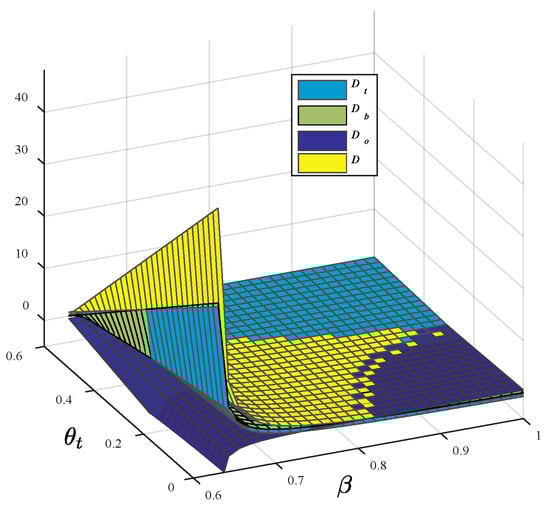
Figure 10.
Demand in Scenario D (1).
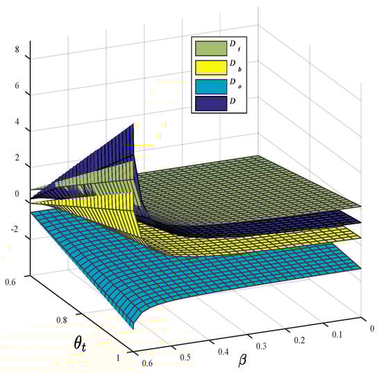
Figure 11.
Demand in Scenario D (2).
As for the sales volume of each distribution channel, when the proportion of traditional consumers is relatively small (), the demands of traditional consumers and BOPS consumers change in the opposite direction with the proportion of cost allocation, while the demand of online shopping consumers changes in the same direction with the cost-sharing ratio as Figure 10 shows. When the ratio of traditional consumers is relatively large (), the changing trend of the demand of each distribution channel with the cost-sharing ratio is converse to the above. The reason is that when the proportion of traditional consumers is relatively high in the initial stage of the deployment of an omnichannel strategy, the cost allocation mechanism promotes the improvement of offline service, which also promotes the transfer of consumers to traditional offline channels and BOPS sales channel. Hence the demands of traditional consumers and BOPS consumers expand. In contrast, the demand of online shopping consumers decreases with the increase in the cost allocation ratio. When the scale of traditional consumers reaches a certain value or even smaller, the expansion of cost allocation proportion conversely results in the decline in traditional consumer’s demand and BOPS consumer’s demand. In this case, the cost allocation mechanism cannot stimulate the demands in the traditional offline and BOPS sales channel. Based on the changes of sales volume in various channels, it can be included that the demand for the retail system expands with the increase in the cost allocation ratio when the proportion of traditional consumers is relatively high. At the same time, the gross demand declines as the cost allocation ratio increases when the proportion of traditional consumers is relatively small. To maximize the gross demand, retail enterprises should encourage the online platform to undertake service costs as many as possible in the early stage of omnichannel retail development and then reduce the cost-sharing proportion with the gradual expansion of the online shopping consumers and BOPS consumers.
Proposition 7.
In the BOPS model dominated by the brick-and-mortar store,
- (i)
- The profit of the online platformincreases with the cost-sharing ratiowhenor, and decreases within other cases.
- (ii)
- The profit of the brick-and-mortar storeincreases with the cost-sharing ratio.
- (iii)
- The profit of the retail systemincreases with the cost-sharing ratiowhen, and decreases withotherwise.
Proposition 7 displays the changes in profits of the online platform, the brick-and-mortar store, and the retail system with the proportion of cost allocation. When both the cost-sharing ratio and the proportion of traditional consumers are relatively small or large, the profit of the online platform increases with the cost-sharing ratio. In other cases, the profit for the online platform decreases with the cost-sharing ratio. In contrast, the profit of the brick-and-mortar store always increases as the cost-sharing proportion increases. This conclusion also implies that in the omnichannel retail supply chain dominated by the brick-and-mortar store, the cost allocation mechanism of offline service is always beneficial to the offline retailer. At the same time, the online platform needs to intensely observe the composition of consumers in the market and choose the optimal cost allocation ratio according to the scale of traditional consumers. In the whole retail system, the gross profit increases with the rise of the cost allocation ratio when the proportion of traditional consumers is relatively small (), while the gross profit declines as the cost allocation ratio increases when the proportion of traditional consumers is relatively high (). The change rule of gross profit implies that, for the profit of the whole retail system, the enthusiasm of the online platform to improving the quality of service should be greatly mobilized when the scale of traditional consumers is large. In the omnichannel retail supply chain dominated by the brick-and-mortar store, the profits of the online platform and the retail system are affected by the proportion of traditional consumers and the cost allocation ratio simultaneously.
Figure 12 and Figure 13 visually depict the changes in the profit of the retail system with a cost-sharing ratio. Figure 12 portrays the profit of the retail system by setting , and . In this case, the proportions of traditional consumers , , and are always larger than , and the profit of the retail system increases with the cost sharing ratio as shown in Figure 12. Figure 13 shows that by setting , , and , the proportion of traditional consumers , , and are smaller than the minimum of , the profit of the retail system decreases with the cost sharing ratio in these cases as P7 demonstrates.
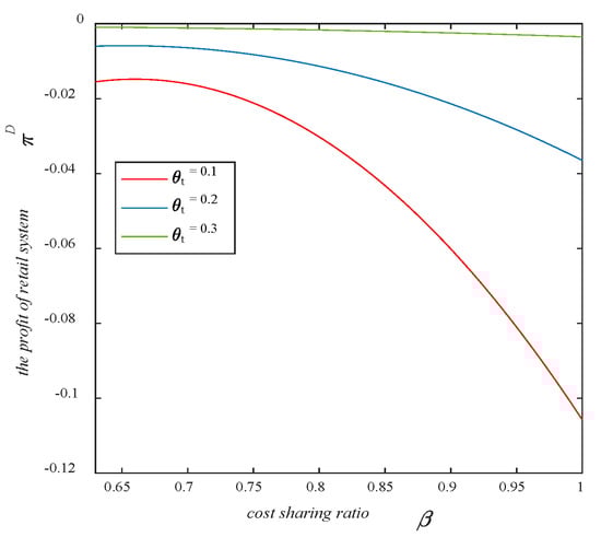
Figure 12.
Profit of retail system in Scenario D (1).
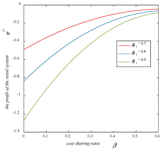
Figure 13.
Profit of retail system in Scenario D (2).
6.2. Insights on the Proportion of Traditional Consumers
Proposition 8.
In the BOPS model dominated by the brick-and-mortar store,
- (i)
- Pricedecreases with the proportion of traditional consumersin the threshold, and increases within the threshold.
- (ii)
- Service levelincreases with the proportion of traditional consumerswhen, and decreases withotherwise.
By setting , , and , Figure 14 and Figure 15 graphically depict the variations of the sales price and service level with the proportion of traditional consumers when and separately. In the case of , we can obtain from Figure 14 that the service level increases with the traditional consumer share, but the sales price decreases with the traditional consumer share when and increases with the traditional consumer when . In the case of , it can be observed from Figure 15 that both the service level and sales price decrease with the proportion of traditional consumers. Proposition 8 shows that in the omnichannel retail supply chain dominated by the brick-and-mortar store, the cost allocation ratio and the proportion of traditional consumers influence the uniform price and the level of service jointly. When the proportion of cost allocation is relatively small or large, that is or , the uniform price increases with the decline in the proportion of traditional consumers. When the cost allocation ratio is in the range , the uniform price decreases with the decline in the proportion of traditional consumers. While for the level of service, as the proportion of traditional consumers declines, the service level decreases when the cost-sharing ratio is relatively small () and increases when the cost-sharing ratio is relatively large (). The reason is that, in the retail system dominated by the brick-and-mortar store, when the online platform is less motivated to undertake part of the offline service cost, which means the cost allocation ratio is relatively small, the service enthusiasm of the brick-and-mortar store also decreases with the reduction in the scale of traditional consumers. In contrast, when the cost allocation ratio is relatively high, the offline store chooses to improve the quantity of service to reduce customer’s concern under the cost allocation mechanism. As the proportion of traditional consumers declines, the improvement of service level results in the growth of operating costs. Thus, the uniform retail price increases accordingly.
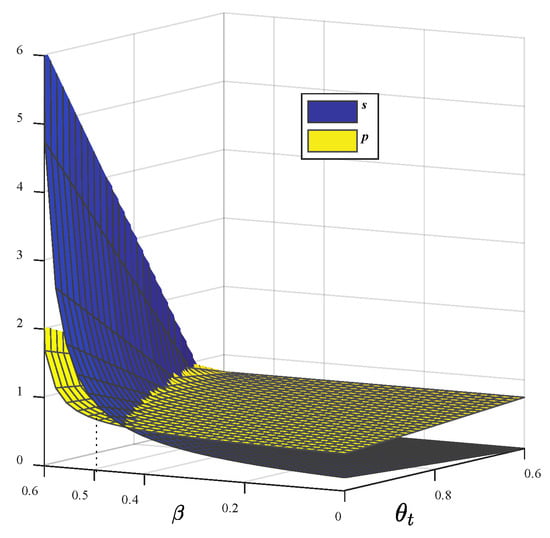
Figure 14.
Price and service in Scenario D (3).
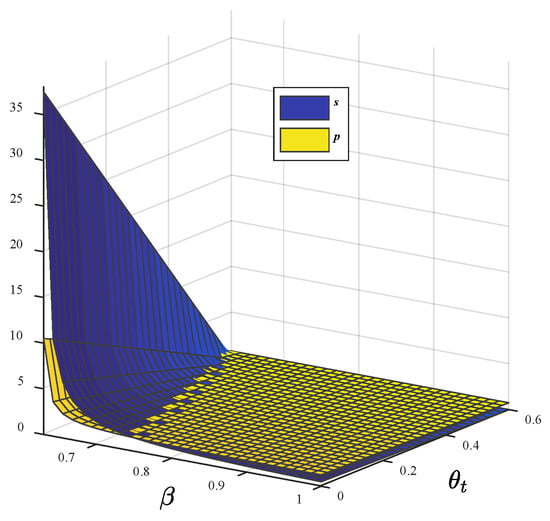
Figure 15.
Price and service in Scenario D (4).
Proposition 9.
In the BOPS model dominated by the brick-and-mortar store,
- (i)
- Traditional consumers’ demandincreases with the proportion of traditional consumersin the threshold, and decreases within the threshold.
- (ii)
- BOPS consumers’ demandincreases with the proportion of traditional consumersin the threshold, and decreases in the threshold.
- (iii)
- Online shopping consumers’ demanddecreases with the proportion of traditional consumersin the threshold, and increases within the threshold.
- (iv)
- The retail system’s demandincreases with the proportion of traditional consumersin the threshold, and decreases in the threshold.
Proposition 9 indicates that the demand of each distribution channel changes with the proportion of traditional consumers in different cost-sharing ratio ranges. In order to reflect the changing trend more intuitively for the demands of different consumers, Table 4 displays the joint influences of the cost allocation ratio and the proportion of traditional consumers on the demand of different consumer groups. It can be included from the table that when the proportion of cost allocation is relatively small () or large (), the gross demand of the retail system decreases with the shrinking of traditional consumers. Only when the cost allocation ratio is in the appropriate range of , does the total demand increase as the proportion of traditional consumers declines. In other words, when the proportion of traditional consumers declines in the initial stage of omnichannel retail development, the retail enterprise should make the cost allocation of the online platform greater than but less than for the maximum gross demand in the retail system.
Table 4.
Variation of demand with the proportion of traditional consumers.
Additionally, the conclusion shows that in the case of , the demands of BOPS consumers, traditional consumers, and the retail system change in the same direction as the proportion of traditional consumers. The reason is that the service level increases with the proportion of traditional consumers when as Proposition 8 demonstrates, consequently the improvement of service promoting the expansion of offline customers scale. Furthermore, the demands of various groups of consumers all change in the opposite direction as the scale of traditional consumers increases when the cost allocation ratio is greater than and less than . When the proportion of traditional consumers ranges in , the demands of online shopping consumers, BOPS consumers, and traditional consumers all increase with the decline in the proportion of traditional consumers. This conclusion implies that both the online platform and the brick-and-mortar store wish the ratio of cost allocation to be greater than and less than . Comprehensively considering the gross demand of the retail system and the stabilities of the online platform and offline store, the optimal range of the cost allocation ratio is as the proportion of traditional consumers declines in the initial stage of the development of omnichannel retail.
Proposition 10.
In the BOPS model dominated by the brick-and-mortar store,
- (i)
- The profit of the online platformdecreases with the proportion of traditional consumerswhenoror, and increases within other cases.
- (ii)
- The profit of the brick-and-mortar storeincreases with the proportion of traditional consumerswhenoror, and decreases within other cases.
- (iii)
- The profit of the retail systemincreases with the proportion of traditional consumerswhen, and decreases withotherwise.
It can be concluded from this proposition that the changes in profits of the online platform and the brick-and-mortar store with the proportion of traditional consumers are related to the cost allocation ratio. When both the cost-sharing ratio and the proportion of traditional consumers are relatively small, the profit of the online platform decreases with the proportion of traditional consumers. In contrast, the profit of the brick-and-mortar store increases. Conversely, the profit of the online platform increases with the scale of traditional consumers, and the profit of the brick-and-mortar store decreases with the scale of traditional consumers when the cost-sharing ratio and the proportion of traditional consumers are relatively large. In addition, the profit of the retail system first increases and then decreases with the proportion of traditional consumers. The conclusion also implies there is an optimal proportion of traditional consumers , which maximizes the profit of the retail system. The enlightenment of this conclusion is that retail enterprises need to control the scale of various types of consumers to maximize profits through the omnichannel retail strategy, which also shows that the development of omnichannel retail cannot blindly squeeze the share of demand of traditional channels.
7. Comparative Analysis
Scenario U and Scenario D respectively display the pricing and service decisions of the online platform and the brick-and-mortar store, the demand of various consumers, and the profits for different entities in the retail system under the cost allocation mechanism of omnichannel retail strategy. In order to further explore the influences of different power structures on omnichannel retail decision-making, the following part of the study explores pricing and service decisions and the profits of retail entities under different scenarios.
Proposition 11.
Comparing Scenario U and Scenario D,
- (i)
- Service levelin Scenario U is higher thanin Scenario D whenor, and lower thanin other cases.
- (ii)
- Pricein Scenario U is higher thanin Scenario D whenor, and lower thanin other cases.
Proposition 11 indicates that comparing service levels under different power structures is determined by combining cost-sharing ratios and traditional consumers’ proportions. When both the cost-sharing ratio and the proportion of traditional consumers are small or large, the service level is higher under the online platform-led omnichannel retail model than that in the offline store-led omnichannel retail model. However, in other cases, the service level is higher in the offline store-led omnichannel retail model. Additionally, the uniform price and the demand of online shopping consumers are also influenced by the combination of the cost-sharing ratio and the proportion of traditional consumers. When both the cost-sharing ratio and proportion of traditional consumers are small or large, the uniform price in an online platform-led omnichannel retail supply chain is higher than that in brick-and-mortar store-led omnichannel retail supply chain, hence the former online shopping consumer demand is smaller than the latter. In other cases, the contrast between the magnitude of the uniform retail price and online shopping consumers’ demand under the two dominant models is the opposite of the above.
Proposition 12.
Comparing Scenario U and Scenario D,
- (i)
- The demand of online shopping consumersin Scenario U is lower thanin Scenario D whenor, and higher thanin other cases.
- (ii)
- The demand of traditional consumersand the demand of BOPS consumersin Scenario U are respectively higher thanandin Scenario D whenoror, and the contrast is reversed in other cases.
- (iii)
- The demand for the retail systemin Scenario U is higher thanin Scenario D whenoror.
It can be concluded from Proposition 12 that the demand of online shopping consumers is also influenced by the combination of the cost-sharing ratio and the proportion of traditional consumers. When both the cost-sharing ratio and proportion of traditional consumers are relatively small or large, the uniform price in the online platform-led omnichannel retail supply chain is higher than that in brick-and-mortar store-led omnichannel retail supply chain as Proposition 11 shows, therefore the former online shopping consumer demand is smaller than the latter. In other cases, the contrast between the magnitude of the uniform retail price and online shopping consumers’ demand under the two dominant models is the opposite of the above. The laws of variation of the demand of traditional consumers, BOPS consumers, and the retail system with the proportion of traditional consumers are more complex. When the cost-sharing ratio and the proportion of traditional consumers are relatively small, the demands of various consumer groups are higher in Scenario U than those in Scenario D.
Proposition 13.
Comparing Scenario U and Scenario D,
- (i)
- Supposing the two solutions ofareandrespectively, then, and the solution of is, which can be calculated as 0.728177. The profit of the online platformin Scenario U is higher thanin Scenario D whenoror, and lower thanin other cases.
- (ii)
- Supposing the two solutions ofareandrespectively, then. The profit of the brick-and-mortar storein Scenario U is higher thanin Scenario D whenor, and lower thanin other cases.
- (iii)
- Supposing the two solutions of are and respectively, then and the solution of is , which can be calculated as 0.412334. The profit of the retail system in Scenario U is higher than in Scenario D when or or or , and lower than in other cases.
Proposition 13 displays the composition of the profit of each entity in the two scenarios. It can be concluded from (i) that when the cost-sharing ratio is relatively high (), only when the traditional consumers’ share is moderate () does the online platform become more profitable in the retail system dominated by itself. When the cost-sharing ratio is relatively small, the profit of the online platform is higher in the system dominated by itself in the case where the proportion of traditional is in the threshold of or . It is obvious that in the retail system dominated by the online platform, the online platform prefers to reduce cost sharing ratio as many as possible to increase the potential for more profits. However, when the brick-and-mortar store dominates the retail system, the online platform is expected to undertake more service costs. This finding reflects the influence of power structures on supply chain members’ decisions. Proposition 13 (ii) demonstrates that when the cost-sharing ratio is relatively high (), the brick-and-mortar store is more profitable in the retail system dominated by the online platform than that dominated by itself. However, when the cost-sharing ratio is relatively small, only when the proportion of traditional consumers is moderate () does the brick-and-mortar store become more profitable in the system dominated by the online platform, which means that when the cost-sharing ratio is relatively high, the brick-and-mortar store prefers to choose the retail system dominated by the online platform.
Table 5, Table 6 and Table 7 show the comparisons of profits under different dominant powers. It could be concluded from the (iii) that the profit of the retail system dominated by the online platform is higher than that dominated by the brick-and-mortar store when the cost-sharing ratio is relatively high () considering the profits of the online platform and the brick-and-mortar store. This conclusion indicates that the profit of the overall system is higher in the online platform-led retail system than that in the brick-and-mortar store-led retail system with a relatively high-cost sharing ratio, and the conclusion is reversed when the cost-sharing ratio is relatively small. Therefore, to maximize the system’s profit, it is recommended to increase the cost-sharing ratio when the online platform dominates the retail system and decreases the cost-sharing ratio when the brick-and-mortar store dominates, which also reflects the checks and balances on power.
Table 5.
The comparison of online platform’s profit between Scenario U and Scenario D.
Table 6.
The comparison of brick-and-mortar store’s profit between Scenario U and Scenario D.
Table 7.
The comparison of retail system’s profit between Scenario U and Scenario D.
8. Managerial Implications and Conclusions
This paper conducts a theoretical analysis of BOPS omnichannel retail under the cost allocation mechanism concerning power structure. According to the power structure of retail supply chain, two scenarios under the cost-sharing mechanism are constructed to explore the operational strategies, which are the BOPS model dominated by the online platform and the BOPS model dominated by the brick-and-mortar store. The influences of cost sharing and the scale of traditional consumers on operational strategies and the profit of each supply chain entity are examined. In addition, the operational strategies, the demands of different distribution channels, and the profit of each retail entity in the two power structures are compared. The main findings and managerial insights are highlighted as below.
In terms of the cost-sharing ratio, its impacts on the decision-making and profit of each entity are systematically analyzed. In the omnichannel retail supply chain dominated by online retailer, the online platform has a first-moving advantage in decision-making. To a certain extent, the increase in the cost-sharing ratio motivates the brick-and-mortar store to improve its service. However, the service level decreases with the cost-sharing ratio when it is relatively high. With the increase in the cost-sharing ratio, the total demand of the retail system first increases and then decreases, but the profit of the online platform first increases and then decreases. From the perspective of the online platform, it is not willing to continuously increase the cost-sharing ratio based on its own profit. In contrast, in the retail system dominated by the brick-and-mortar store, the service level, the total demand, and the total profit of the retail system only increase with the cost-sharing ratio when the scale of traditional consumers is relatively high. This conclusion demonstrates that in the initial stage of omnichannel retail, the scale of traditional consumers is relatively large, and the performance of the retail system can be effectively improved by increasing the cost-sharing ratio. However, when the scale of traditional consumers shrinks to a certain size, the cost-sharing mechanism cannot contribute to the profit of the retail system.
In addition, it is found that consumer composition significantly influences the decision-making and profit of the omnichannel retail supply chain based on the study of traditional consumer proportion. In the omnichannel retail supply chain dominated by online retailer, the service level decreases with the proportion of traditional consumers. With the increase in the proportion of traditional consumers, all the profits of the online platform, the brick-and-mortar store and the retail system first increase and then decrease. This result demonstrates that the efficient implementation of an omnichannel retail strategy does not compress the traditional consumers’ consumption space. In the retail system dominated by brick-and-mortar stores, the service level only increases with the proportion of traditional consumers when the cost-sharing ratio is relatively small. The profit of the retail system first increases and then decreases with the proportion of traditional consumers. The two retail systems under different power structures are compared, and when the cost-sharing ratio and the proportion of traditional consumers are relatively small, the service level, the uniform price, and the total demand in the retail system dominated by the online platform are higher.
Considering the impact of the cost-sharing mechanism and the consumer composition synchronously, several managerial insights and practical observations can be made regarding omnichannel retail.
For online platforms that dominate the retail system, which are represented by e-commerce platforms trying to realize omnichannel retail by laying out offline stores: (1) Bearing part of the service costs does not always undermine their profitability. In contrast, sharing an appropriate proportion of service costs is not only conductive for cross-channel cooperation, but also can improve their profit. In particular, the profit of online platforms reaches its highest level when the cost-sharing ratio equals 1/3, which is considered to be the optimal ratio of cost-sharing for online platforms. (2) As the dominant party in the retail system, online platforms tend to try their best to capture the share of demand, because the increasing proportion of traditional consumers is always detrimental to online platforms although omnichannel retailing is beneficial to the development of brands.
For brick-and-mortar stores dominate the retail system, which are represented by offline physical stores trying to realize omnichannel retail by expanding online channels: (1) As the dominant party in the retail system, the brick-and-mortar stores tend to pressure online platforms to bear as many of the service costs as possible, as the increased cost share of online platforms always enhances the profitability of the brick-and-mortar stores. Considering the profitability of online platforms, when both the cost-sharing ratio and the proportion of traditional consumers are relatively large, the profit of online platforms increases with the cost-sharing ratio. Therefore, in the initial stage of channel integration, when the proportion of traditional consumers is relatively large, the brick-and-mortar stores should cooperate with online platforms to set up cost-sharing contracts, so that both parties can profit from the increase of cost-sharing ratio and the retail system supply chain will be in a stable state. (2) The expansion of traditional consumers scale is not always beneficial to brick-and-mortar stores, and the impact of traditional consumers’ proportion on brick-and-mortar stores’ profits is affected by the combination of cost-sharing ratios and traditional consumers share.
For retail corporations deploying the BOPS strategy, (1) The development of omnichannel retail cannot continue to squeeze traditional consumers’ consumption channels, as the profit of the retail system always first increases and then decreases with the proportion of traditional consumers. (2) When the cost-sharing ratio stipulated in the cooperation contract between online platforms and brick-and-mortar stores is relatively large, specifically greater than 1/2, the profit of the retail system dominated by online platforms is higher compared to that dominated by brick-and-mortar stores. This means that for the whole retail system, the cost-sharing pressure on the online platforms is best to match with their channel power.
However, our study still has limitations in terms of research methodology and research scope. First, the article assumes that consumers’ demand divisions in different channels are known, and fails to delicately portray consumers’ choice and transfer behavior among channels according to their own utilities. Second, our study ignores the possible phenomenon of “Showrooming” or “Webrooming” in omnichannel retail, which will have influence on consumers’ behavior. Based on this, the next step of research is to add consumer utility theory to the study to explore the supply chain coordination strategies in the phenomenon of “Showrooming” and “Webrooming” in order to become more scientific and instructive conclusions.
Author Contributions
Methodology, Y.G.; software, Z.W.; investigation, Y.G.; writing—orignal draft preparation, Y.M. All authors have read and agreed to the published version of the manuscript.
Funding
This research was funded by National Natural Science Foundation of China (72102112), the Ministry of education of Humanities and Social Science project (22YJA630022), and Qinglan Project of Jiangsu University.
Data Availability Statement
Not applicable.
Acknowledgments
The authors would like to thank Yue WANG for her polishing the English language and style.
Conflicts of Interest
The authors declare no conflict of interest.
Appendix A
Proof of Proposition 1.
Since , and hold, we can acquire . By the game equilibrium results of Scenario U, we can obtain . Since and hold, we can obtain that only when can we acquire , thence ; only when can we acquire . Similarly, for , only when can we acquire , thence ; only when can we acquire . □
Proof of Proposition 2.
Based on the game equilibrium results of Scenario U, we can obtain , as well as , and hold. Only when can we acquire , thence and ; conversely, we have and when . As for , when , we have , thence . In contrast, when , we have . As for , we can check that when , ; when , . □
Proof of Proposition 3.
Based on the game equilibrium results of Scenario U, we can obtain . Only when can we acquire , thence ; only when can we acquire . As for and , we can check that and hold. When , we have ; when , we have . In contrast, we can acquire only when ; when , we can acquire .
Additionally, , . □
Proof of Proposition 4.
Based on the game equilibrium results of Scenario U, we can obtain . Since and hold, thus . Similarly, we can acquire , . For and , since and hold, and . For , holds, and we can obtain that only when can we acquire , thence . Conversely, we can acquire only if . □
Proof of Proposition 5.
Based on the game equilibrium results of Scenario U, we can acquire . Since and hold, thus . For , we can check that holds. Only when can we acquire , thence . Conversely, only when can we acquire . As for , we can check that holds when , therefore we have , thence . Conversely, when , we have . □
Proof of Proposition 6.
Based on the game equilibrium results of Scenario D, we can obtain ,
, , , and . When , we have , thence , , , , and ; Conversely, when , we have , , , , and . □
Proof of Proposition 7.
(i) Based on the game equilibrium results of Scenario D, we can acquire . In addition, we can acquire since . From the equation, we can find only if .
Case 1. When , holds. In this case, only when can we acquire , thence . Conversely, only when can we acquire .
Case 2. When , holds. In this case, we can check that when , thence . In contrast, we have when .
(ii) Based on the game equilibrium results of Scenario D, we can acquire . In addition, we can acquire since . From the equation, we can find that only if . Only when can we acquire , thence . Conversely, only when can we acquire . □
Proof of Proposition 8.
(i) Based on the game equilibrium results of Scenario D, we can acquire . From the equation, we can find that only when can we acquire ,and only when or can we acquire . (ii) Based on the game equilibrium results of Scenario D, we can acquire . Therefore, when , we have ; when , we have . □
Proof of Proposition 9.
(i) Based on the game equilibrium results of Scenario D, we can acquire . From the equation, we can find that only if or , and only if . (ii) From the equation , we can find that only when can we acquire , and only when
, can we acquire . (iii) As for , when , we have ; when or ,we have . (iv) From the equation , we can acquire that when or ,we have ;when , we have . □
Proof of Proposition 10.
(i) Based on the game equilibrium results of Scenario D, we can acquire . From the equation, we can find that if and only if .
Case 1. When or , holds. In this case, only when can we acquire , thence ; Conversely, only when can we acquire .
Case 2. When , holds. In this case, only when can we acquire , thence ; Conversely, only when can we acquire .
(ii) Based on the game equilibrium results of Scenario D, we can acquire . From the equation, we can find that only if both and are positive or negative.
Case 1. When , and hold. In this case, only when can we acquire and , thence ; Conversely, only when can we acquire .
Case 2. When , and hold. In this case, only when can we acquire and , thence ; Conversely, only when can we acquire .
Case 3. When , and hold. In this case, only when can we acquire and , thence ; Conversely, only when can we acquire .
(iii) Based on the game equilibrium results of Scenario D, we can acquire . From the equation, we can find that only if . Since holds, only when can we acquire , thence ; Conversely, only when can we acquire . □
Proof of Proposition 11.
(i) Based on the optimal solutions of Scenario U and Scenario D, we can acquire . From the equation, we can find that only if both and are positive or negative.
Case 1. When , , and hold. In this case, only when can we acquire and , thence ; Conversely, when , we have .
Case 2. When , , and hold. In this case, only when can we acquire and , thence ; in contrast, when , we have .
(ii) Based on the optimal solutions of Scenario U and Scenario D, we can acquire . From the equation, we can find that only if both and are positive or negative.
Case 1. When , , and hold. In this case, only when can we acquire and , thence ; Conversely, when , we have .
Case 2. When , ,
and hold. In this case, only when can we acquire and , thence ; Conversely, when , we have . □
Proof of Proposition 12.
(i) Based on the optimal solutions of Scenario U and Scenario D, we can acquire . From the equation, we can find that only if both and are positive or negative.
Case 1. When , ,
, and hold. In this case, only when can we acquire and , thence ; Conversely, when , we have .
Case 2. When , , and hold. In this case, only when can we acquire and , thence ; Conversely, when , we have .
(ii) Based on the optimal solutions of Scenario U and Scenario D, we can acquire . From the equation, we can find that and only if both and are positive or negative.
Case 1. When , , and hold. In this case, only when can we acquire and , thence and ; Conversely, when , we have and .
Case 2. When , , and hold. In this case, only when can we acquire and , thence and ; Conversely, when , we have and .
Case 3. When , , and hold. In this case, only when can we acquire , thence
and ; Conversely, when , we have and .
(iii) Based on the optimal solutions of Scenario U and Scenario D, we can acquire . From the equation, we can find that
only if both and are positive or negative.
Case 1. When , , and hold. In this case, only if can we acquire and ,
thence; ; Conversely, only if can we acquire .
Case 2. When , , and hold. In this case, only if can we acquire and , thence ; Conversely, only if can we acquire .
Case 3. When, , , and hold. In this case, only if can we acquire and , thence . Conversely, only if can we acquire . □
Proof of Proposition 13.
(i) Based on the optimal solutions of Scenario U and Scenario D, we can acquire . From the equation, we can find that only if since hold. Considering the numerator as a quadratic function with respect to , , and . The discriminant equation holds. Assuming , then we can acquire and holds, which means the function monotonically decreases. Assuming , the solutions of are and , and . Next, according to the image characteristics of quadratic functions, we can acquire:
Case 1. When , holds, so the quadratic function is U-shaped. In this case, only when or can we acquire , thence ; and only when can we acquire .
Case 2. When , holds, so the quadratic function is inverted U-shaped. In this case, only when can we acquire , thence ; and only when or can we acquire .
By calculating, we can acquire
, , .
(ii) Based on the optimal solutions of Scenario U and Scenario D, we can acquire . From the equation, we can find that only if and are both positive or negative. Considering the numerator as a quadratic function with respect to , , , and . According to the discriminant equation , we can obtain that only if can we acquire in the threshold of , thence ; only if can we acquire . Assuming , then we can acquire , , and holds, which means function monotonically increases.
Case 1. Since monotonically increases and in the threshold of , which means monotonically increases in the threshold of . Since and increases in the threshold of , holds, indicating the quadratic function is U-shaped. Since and in the threshold of , . Since and , we have .
Case 2. Since monotonically increases and and function monotonically decreases first and then increases, and the minimum is (). Therefore holds, which means the quadratic function is U-shaped. Assuming the solutions of are and , and , according to the image characteristics of the quadratic function, we can obtain that: only when can we acquire and , thence ; Similarly, only when or can we acquire and , thence .
By calculating, we can acquire
, , .
(iii) Based on the optimal solutions of Scenario U and Scenario D, we can obtain . From the equation, we can find that only if since holds.
Considering the numerator as a quadratic function with respect to , we have , , and .
From the discriminant equation , we can obtain that only if can we acquire in the threshold of , thence ; only if can we acquire . Assuming , then we can acquire , , , and holds.
Case 1. When , holds, which means the function monotonically increases. Since , , , indicating that monotonically decreases in the threshold of . Since , and , we can acquire , which means monotonically increases. Since and , we assume . when and when . Assuming the solutions of are and , . According to the image characteristics of quadratic functions, we can acquire: (1) when , holds. In this case, only when can we acquire , thence ; And only when or can we acquire . (2) when , holds. In this case, when or , we have , thence ; when , we have .
Case 2. When , holds, which means the quadratic function is U-shaped. Since and , , so we have .
By calculating, we can acquire
, . □
References
- Jindal, R.P.; Gauri, D.K.; Li, W.; Ma, Y. Omnichannel battle between Amazon and Walmart: Is the focus on delivery the best strategy? J. Bus. Res. 2021, 122, 270–280. [Google Scholar] [CrossRef] [PubMed]
- Verhoef, P.C.; Kannan, P.K.; Inman, J.J. From multi-channel retailing to omni-channel retailing: Introduction to the special issue on multi-channel retailing. J. Retail. 2015, 91, 174–181. [Google Scholar] [CrossRef]
- Saghiri, S.; Wilding, R.; Mena, C.; Bourlakis, M. Toward a three-dimensional framework for omni-channel. J. Bus. Res. 2017, 77, 53–67. [Google Scholar] [CrossRef]
- Li, H.; Yang, S.; Kang, H.; Shi, V. “Buy online, pick up in store” under fit uncertainty: To offer or not to offer. Complexity 2020, 2020, 3095672. [Google Scholar] [CrossRef]
- Zhang, Q.; Cao, W.; Liu, Y.; Zhang, Z. Integration of online and offline channels in retail: Feasibility of BOPS? Kybernetes 2021, 50, 1588–1620. [Google Scholar] [CrossRef]
- Gallino, S.; Moreno, A.; Stamatopoulos, I. Channel integration, sales dispersion, and inventory management. Manag. Sci. 2017, 63, 2813–2831. [Google Scholar] [CrossRef]
- Gao, F.; Su, X. Omnichannel retail operations with buy-online-and-pick-up-in-store. Manag. Sci. 2017, 3, 2478–2492. [Google Scholar] [CrossRef]
- Lu, J.C.; Yang, Y.; Han, S.Y.; Tsao, Y.C.; Xin, Y. Coordinated inventory policies for meeting demands from both store and online BOPS channels. Comput. Ind. Eng. 2020, 145, 106542. [Google Scholar] [CrossRef]
- Jiang, Y.; Liu, L.; Lim, A. Optimal pricing decisions for an omni-channel supply chain with retail service. Int. Trans. Oper. Res. 2020, 27, 2927–2948. [Google Scholar] [CrossRef]
- Liu, J.; Xu, Q. Joint decision on pricing and ordering for omnichannel bops retailers: Considering online returns. Sustainability 2020, 12, 1539. [Google Scholar] [CrossRef]
- Li, M.; Zhang, X.; Dan, B. Cooperative advertising and pricing in an O2O supply chain with buy-online-and-pick-up-in-store. Int. Trans. Oper. Res. 2021, 28, 2033–2054. [Google Scholar] [CrossRef]
- Shen, X.L.; Li, Y.J.; Sun, Y.; Wang, N. Channel integration quality, perceived fluency and omnichannel service usage: The moderating roles of internal and external usage experience. Decis. Support Syst. 2018, 109, 61–73. [Google Scholar] [CrossRef]
- Pauwels, K.; Neslin, S.A. Building with bricks and mortar: The revenue impact of opening physical stores in a multichannel environment. J. Retail. 2015, 91, 182–197. [Google Scholar] [CrossRef]
- Wang, R.J.H.; Malthouse, E.C.; Krishnamurthi, L. On the go: How mobile shopping affects customer purchase behavior. J. Retail. 2015, 91, 217–234. [Google Scholar] [CrossRef]
- Hsiao, L.; Chen, Y.J. Strategic motive for introducing internet channels in a supply chain. Prod. Oper. Manag. 2014, 23, 36–47. [Google Scholar] [CrossRef]
- Zhang, P.; He, Y.; Shi, C.V. Retailer’s channel structure choice: Online channel, off-line channel, or dual channels? Int. J. Prod. Econ. 2017, 191, 37–50. [Google Scholar] [CrossRef]
- Hu, M.; Xu, X.; Xue, W.; Yang, Y. Demand pooling in omnichannel operations. Manag. Sci. 2022, 68, 883–894. [Google Scholar] [CrossRef]
- Jin, M.; Li, G.; Cheng, T.C.E. Buy online and pick up in-store: Design of the service area. Eur. J. Oper. Res. 2018, 268, 613–623. [Google Scholar] [CrossRef]
- Zhou, Y.W.; Guo, J.; Zhou, W. Pricing/service strategies for a dual-channel supply chain with free riding and service-cost sharing. Int. J. Prod. Econ. 2018, 196, 198–210. [Google Scholar] [CrossRef]
- Chakraborty, A.; Mateen, A.; Chatterjee, A.K.; Haldar, N. Relative power in supply chains–Impact on channel efficiency & contract design. Comput. Ind. Eng. 2018, 122, 202–210. [Google Scholar]
- Fan, J.; Ni, D.; Fang, X. Liability cost sharing, product quality choice, and coordination in two-echelon supply chains. Eur. J. Oper. Res. 2020, 284, 514–537. [Google Scholar] [CrossRef]
- Chen, X.; Zhou, J. The complexity analysis and chaos control in omni-channel supply chain with consumer migration and advertising cost sharing. Chaos Solitons Fractals 2021, 146, 110884. [Google Scholar] [CrossRef]
- Schul, P.L.; Pride, W.M.; Little, T.L. The impact of channel leadership behavior on intrachannel conflict. J. Mark. 1983, 47, 21–34. [Google Scholar] [CrossRef]
- Kong, R.; Luo, L.; Chen, L.; Keblis, M.F. The effects of BOPS implementation under different pricing strategies in omnichannel retailing. Transp. Res. Part E Logist. Transp. Rev. 2020, 141, 102014. [Google Scholar] [CrossRef]
- Li, X.; Li, Y.; Cao, W. Cooperative advertising models in O2O supply chains. Int. J. Prod. Econ. 2019, 215, 144–152. [Google Scholar] [CrossRef]
- Yan, N.; Liu, Y.; Xu, X.; He, X. Strategic dual-channel pricing games with e-retailer finance. Eur. J. Oper. Res. 2020, 283, 138–151. [Google Scholar] [CrossRef]
- Matsui, K. Power structure and profitability in a three-echelon supply chain facing stochastic demand. Comput. Ind. Eng. 2021, 160, 107246. [Google Scholar] [CrossRef]
- Balakrishnan, A.; Sundaresan, S.; Zhang, B. Browse-and-switch: Retail-online competition under value uncertainty. Prod. Oper. Manag. 2014, 23, 1129–1145. [Google Scholar] [CrossRef]
- Bell, D.R.; Gallino, S.; Moreno, A. Off-line showrooms in omnichannel retail: Demand and operational benefits. Manag. Sci. 2018, 64, 1629–1651. [Google Scholar] [CrossRef]
- Martín-Herrán, G.; Sigué, S.P. Trade deals and/or on-package coupons. Eur. J. Oper. Res. 2015, 241, 541–554. [Google Scholar] [CrossRef]
- Li, G.; Li, L.; Sun, J. Pricing and service effort strategy in a dual-channel supply chain with showrooming effect. Transp. Res. Part E Logist. Transp. Rev. 2019, 126, 32–48. [Google Scholar] [CrossRef]
- Nie, J.; Zhong, L.; Yan, H.; Yang, W. Retailers’ distribution channel strategies with cross-channel effect in a competitive market. Int. J. Prod. Econ. 2019, 213, 32–45. [Google Scholar] [CrossRef]
- Yan, S.; Hua, Z.; Bian, Y. Does retailer benefit from implementing “online-to-store” channel in a competitive market? IEEE Trans. Eng. Manag. 2018, 67, 496–512. [Google Scholar] [CrossRef]


Publisher’s Note: MDPI stays neutral with regard to jurisdictional claims in published maps and institutional affiliations. |
© 2022 by the authors. Licensee MDPI, Basel, Switzerland. This article is an open access article distributed under the terms and conditions of the Creative Commons Attribution (CC BY) license (https://creativecommons.org/licenses/by/4.0/).