A Collision Reduction Adaptive Data Rate Algorithm Based on the FSVM for a Low-Cost LoRa Gateway

Abstract

LoRa (Long Range), a wireless communication technology for low power wide area networks (LPWANs), enables a wide range of IoT applications and inter-device communication, due to its openness and flexible network deployment. In the actual deployment and operation of LoRa networks, the static link transmission scheme does not make full use of the channel resources in the time-varying channel environment, resulting in a poor network performance. In this paper, we propose a more effective adaptive data rate (ADR) algorithm for low-cost gateways, we firstly analyze the impact of the different hardware parameters (RSSI, SNR) on the link quality and classify the link quality using the fuzzy support vector machine (FSVM). Secondly, we establish an end device (ED) throughput model and energy consumption model and design different adaptive rate algorithms, according to the different link quality considering both the link-level performance and the MAC layer performance. The proposed algorithm uses machine learning to classify the link quality, which can accurately classify the link quality using a small amount of data, compared to other adaptive rate algorithms, and the link parameter adaptation algorithm can maximize the throughput while ensuring the link stability, by considering the link-level performance and the MAC layer performance, compared to other algorithms. The results show that it outperforms the standard LoRaWAN ADR algorithm in both the single ED and the multi ED scenarios, in terms of the packets reception rate (PRR) and the network throughput. Compared to the LoRaWAN ADR in 32 multi-ED scenarios, the proposed algorithm improves the throughput by 34.12% and packets the reception rate by 26%, significantly improving the network throughput and the packets reception rate.

1. Introduction

Among the many LPWAN technologies, LoRa can meet the demand of large scale and wide coverages, due to its openness and flexibility [1], the LoRa physical layer adopts the linear spread spectrum modulation technology, which can flexibly adjust the data transmission rate through the different transmission parameter configurations [2]. It achieves a long-distance, a long battery life and a large-scale coverage data transmission.

In the LoRa IoT narrowband network with a wide area coverage, in actual operation, the requirements for the channel bandwidth, the ED energy consumption, and the network connection performance are high. Under the time-varying channel environment, the traditional fixed link transmission scheme cannot fully utilize the channel resources, so the network performance will be greatly reduced [3]. The dynamic link control technology refers to adjusting the link parameters, according to the real-time link quality to adapt to the channel changes, improve the network throughput, and reduce the ED energy consumption. The dynamic link control technology precisely controls the link parameters, according to the channel conditions, which can ensure a link stability, optimize the energy consumption, reduce the retransmission probability and improve the network performance of the LoRa networks [1].

Most of the existing studies on the dynamic link control technology of the LoRa network are based on the LoRaWAN network architecture [4,5], and the LoRa gateway chip that usually uses Semtech SX130x. However, low-cost gateways, based on Semtech SX126x/SX127x chips are often used in the actual deployed LoRa private networks [6] and there is no suitable dynamic link control technology for such networks. Most of the existing studies on the dynamic link control technology of the LoRa network are based on LoRaWAN network architecture [7,8], and the LoRa gateway chip is Semtech SX1301 [5,8]. There is no dynamic link control technology suitable for such networks. In this paper, an ED-GW-NS network architecture is used. The end device (ED) sends the packets to the gateway (GW). The gateway transmits the packets to the network server (NS), which is usually deployed in a cloud computing environment, through other communication technologies (Ethernet/3G/4G). Based on such a network architecture, this paper proposes a conflict-reducing adaptive rate algorithm, suitable for low-cost LoRa gateways. Aiming at the problem that the communication quality of the LoRa technology is susceptible to interference and multi-path effects during the long-distance transmission, a data-driven multi-rate link evaluation model was established. Secondly, a link parameter adaptation model is established for the different link qualities to improve the throughput of the actually deployed LoRa network and reduce the packet loss rate. Compared with the traditional adaptive rate algorithm, the proposed algorithm uses machine learning to build a link quality assessment model to quickly and accurately assess the link quality using a small amount of data, and uses the ED throughput model and energy consumption model, combined with the link budget to build a link parameter adaptation model, that takes into account not only the link-level performance and the MAC layer performance, but also the energy consumption.

The remainder of this paper is organized as follows. Section 2 introduces the current research on the adaptive rate algorithm for the LoRa network, Section 3 constructs a link quality classification model using machine learning, and Section 4 constructs an algorithm optimization objective, based on the established ED throughput and energy consumption models, and adapts the optimal link parameters. Validation and analysis of the algorithm is performed in Section 5, and the paper is concluded in Section 6.

2. Related Work

With the further development of communication technology, the limited spectrum resources become particularly precious, and adaptive technology gradually becomes a new research focus in the field of communication [9]. From 2G to 5G, the link adaptive technology has always been a hot research field. For example, the technical standards, such as GSM, TDMA, and IEEE802.11, select different code rates and coding schemes according to the network conditions [10]. In LPWAN, the introduction of the dynamic link control technology is particularly important to ensure the link stability, optimize the energy consumption, reduce the retransmission probability, and improve the network performance [9,11]. The dynamic link control technology includes the following two aspects.

(1) Link quality assessment

(2) Link parameter adaptation

2.1. Link Quality Estimation

The link quality estimation (LQE) mainly includes methods based on the link characteristics, probability estimation, and machine learning. The method based on link characteristics uses the physical layer indicators (RSSI, SNR, LQI) of the link to evaluate the link quality. Fu [12] et al. proposed a link evaluation algorithm, based on the average LQI and the average RSSI, by analyzing a large amount of communication test data, which can improve the speed and accuracy of the communication link evaluation. Based on the probability estimation method, the link quality is evaluated by calculating the packet reception rate (PRR) of the node, over a period of time. De Couto et al. [13] used the expected transmission count (ETX) to estimate the link quality This method calculates the PRR in both the uplink and the downlink directions to estimate the link quality by sending detection packets. The method models the link quality parameters through a machine learning algorithm, and realizes the evaluation of the link quality. Liu et al. [14] used the multi classification link quality estimation mechanism of the fast decision tree, selected the mean value of the RSSI and LQI, in the window as the estimation parameter, divided the link quality into five levels according to the PRR, and estimated the link quality with the RSSI and LQI in the detection data packet.

2.2. Link Parameter Adaptation

The link parameter adaptation is mainly divided into two categories: one is to consider the ED itself, to adaptively adjust the ED link parameters according to the channel quality, to make full use of the channel characteristics, to ensure the link stability, to optimize the transmission rate, and reduce the energy consumption; the other is to combine the overall situation of the network, to optimize the link configuration of the ED, and to optimize the performance of the entire network.

Considering the throughput and energy consumption of the ED itself, the adaptive rate algorithm [15] in LoRaWAN only considers the link reliability and not the network throughput, and the evaluation of the link quality relies on the maximum SNR of the k packets, which has limitations for sparse IoT services and the channel evaluation is more optimistic. In order to ensure the link stability and the throughput of the current ED, in [16], proposes an ED’s parameter configuration strategy to maximize the ED throughput, but the algorithm does not take into account the time-varying nature of the channel in the real-world application environments and cannot dynamically update the link parameters of the ED. Marini R et al. [17] analyzed the adaptive rate algorithm in LoRaWAN and proposed a conflict aware link parameter adaptation algorithm, which only considers the MAC layer performance to minimize the conflict probability between the EDs, and only adjusts the rate, not the transmission power, without considering the link-level performance. Consider the throughput of the entire network, a fair adaptive data rate algorithm (FADR) is proposed in [18], which assigns the different numbers of EDs at the different rate conditions to ensure the fairness of the network and achieve the same conflict probability for all of the EDs. The algorithm is less scalable and causes multiple ED rate adjustments when adding or removing EDs from the network. Sandoval et al. [19] established a throughput model combined with the global network. The algorithm uses reinforcement learning to derive the link parameters of each ED, to maximize the throughput of the whole network, without considering the link connection performance.

Table 1. Comparison of Adaptive Data Rate Techniques.

Ref.	Proposed Solutions	Link Reliability	Throughput	Energy Consumption	Network Scalability	Heterogeneous Network	Computational Complexity
[15]	LoRaWAN ADR	✓			✓		✓
[16]	SAGA		✓	✓		✓
[17]	CA-ADR	✓	✓		✓		✓
[18]	FADR	✓	✓				✓
[19]	RL-ADR		✓			✓
	The proposed method	✓	✓	✓	✓

shows the comparison of the different ADR algorithms.

3. Link Quality Classification

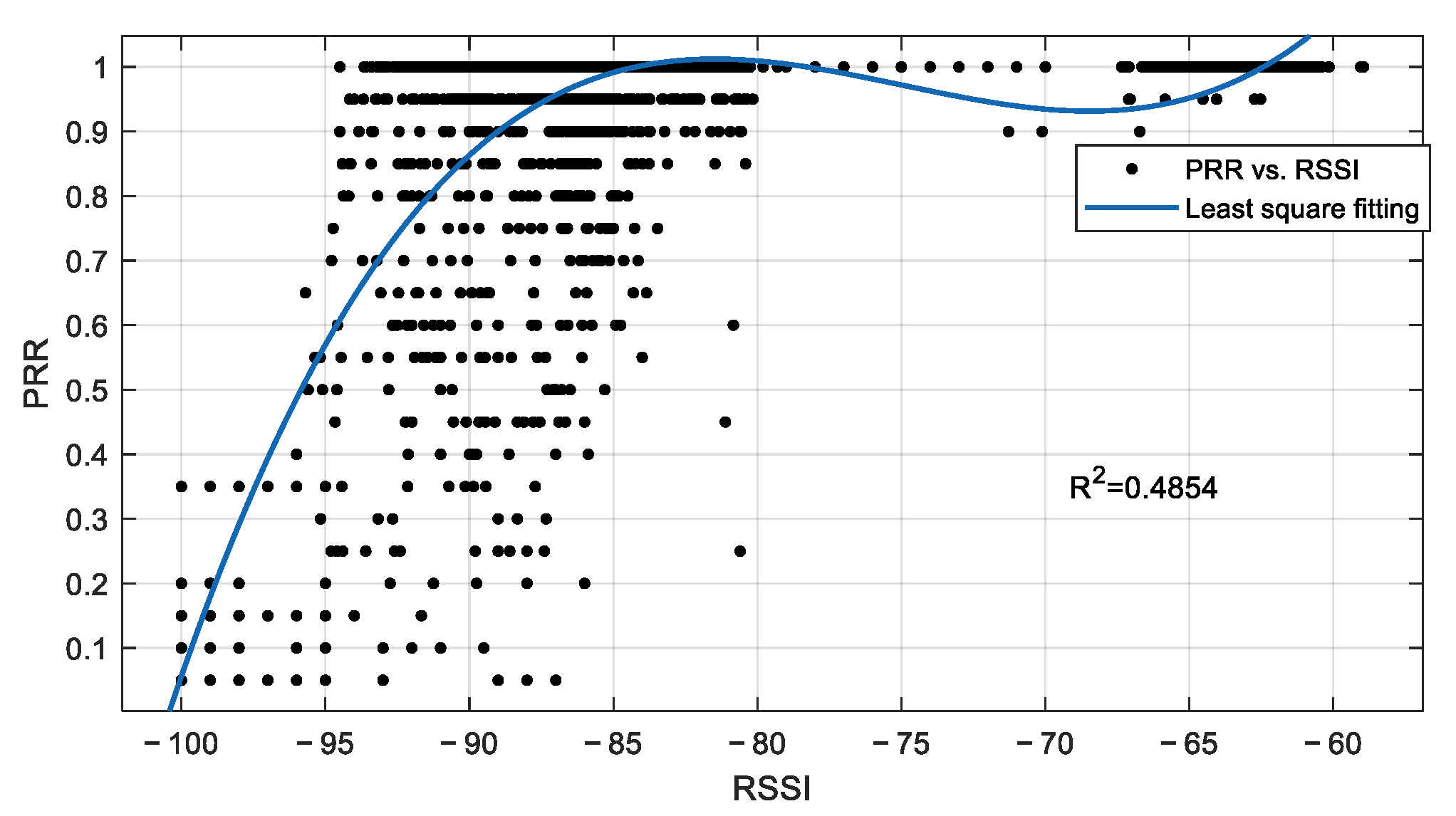
3.1. Link Quality Parameter Selection

Through the analysis of the acquisition of the link quality parameters and the calculation method, it can be seen that the physical layer parameters can be quickly and directly obtained from the device where they are located. The physical layer parameters can reflect the change of the link quality very quickly, with a short acquisition time and a low overhead, but the physical layer parameters are sensitive and fluctuate rapidly [10,17]. PRR, ETX and other parameters of the software layer can more accurately reflect the link quality, but the acquisition time interval is long. The machine learning method is used to divide the link quality level, according to the PRR value, to evaluate the link quality, which not only improves the evaluation accuracy, but also avoids the long-term statistics of the software layer, and reduces the performance of the end devices (EDs), and, to a certain extent, their consumption [11,17]. In order to analyze the relationship between LoRa physical layer indications (SNR, RSSI) and PRR, 71520 packets were collected outdoors using a LoRa terminal with SX1262 RF module, and scatter plots and fitted curves of physical layer indications (SNR, RSSI) and PRR were plotted, the parameter settings are shown in

Table 2. Test parameter configuration.

Parameter	Value
BW	250 KHz
SF	7
Frequency	433 MHz
Packet length	10 Bytes
Transmit power	10 dBm
Preamble length	10

.

The horizontal axis represents the average value of the physical layer indications (RSSI, SNR) of the received data packets with the air time of 20 data packets, as the window length, and the vertical axis represents the PRR (packet reception rate), during the window. The solid line in Figure 1, Figure 2 represents the physical layer indications and the PRR least squared fitting curve, and the goodness of fit R² is obtained.

The closer R² is to 1, the better the fitting degree is, which means the higher the correlation between the physical layer indicators and the PRR. The R² values of the SNR-PRR and the RSSI-PRR are 0.6244 and 0.4854, respectively, indicating that the physical layer indicators (SNR, RSSI) and the PRR provided by the SX1262 chip are related. In this paper, the statistics of the physical layer indicators (RSSI, SNR), are used as the characteristic parameters of the link quality assessment to establish a link quality assessment model combined with machine learning.

Through a large number of practical tests, the link quality deteriorates rapidly in the LoRa networks when the PRR is below 90%, and in the practical applications, the PRR is above 90% to meet the application requirements, so the link quality can be divided into two levels [10,11,20], links with the PRR ∈ [90%, 100%] are classified as good quality links, and PRR ∈ [0, 90%] is divided into bad quality links as Figure 3.

3.2. Theory of Classification Method Based on the FSVM

A support vector machine (SVM) is a two-class model, which usually adopts a one-to-one or one-to-many strategy to convert the multi-class problems into two-class problems. The main idea of a SVM is to construct a geometric interval between two classes. The largest separation hyperplane, its basic model is a linear classifier with the largest interval defined on the feature space, when the data is linearly separable, a method for solving the maximum interval is given; when the data is nonlinearly separable, the original data is mapped into a certain high-dimensional space, the original data is searched for the optimal separating hyperplane in the new dimension, and the point closest to the optimal hyperplane is the support-vector.

The fuzzy support vector machine (FSVM) is an improved SVM, which is realized by introducing a fuzzy membership function, so that different samples have different contributions to the classification hyperplane. The FSVM uses the fuzzy set theory to process the input samples, assigns the different weights to the samples with inconsistent importance, and uses the machine learning method for training and learning, which solves the shortcomings of the standard SVM algorithm that tolerates poor noise, and is suitable for classification problems with noise or outliers. For a set of training samples with a given label, $S={\{(x_i,y_i,s_i)\}}_{i=1}^n$ is the sample point in the input space, and $y_i\in \{+1,-1\}$ is the class label corresponding to the sample. $s_i=[0,1]$ is the fuzzy membership value, which represents the degree to which a sample belongs to a certain class. Consistent with the standard SVM algorithm, the FSVM algorithm also finds a classification hyperplane $w^{\mathrm{T}}\phi (x)+b=0$ that maximizes the classification interval, $w=(w_1,w_2,\cdots ,w_l)$ is a normal vector perpendicular to the classification hyperplane, $b$ is the displacement, and $\phi$ maps the samples $x_i$ from the input space to the feature space. The problem of solving the optimal classification hyperplane in the dimensional space can be transformed into the following optimization problem:

$$\begin{array}{c}\underset{w,b,c}{\min }\frac{1}{2}{\Vert w\Vert }^2+C{\displaystyle \sum _{i=1}^l{s}_i{\epsilon }_i},\\ s.t.\{\begin{array}{c}{y}_i((w^{\mathrm{T}}·\phi (x_i))+b)+{\epsilon }_i\ge 1,i=1,\cdots ,l\\ {\epsilon }_i\ge 0,i=1,\cdots l.\end{array}\end{array}$$

(1)

$\epsilon ={({\epsilon }_1,\cdots ,{\epsilon }_l)}^{\mathrm{T}}$ is the relaxation variable, $C>0$ is a regularization parameter that maintains a balance between the maximum classification interval and the classification error, and $s_i{\epsilon }_i$ is a measure of the degree of misclassification for the variables of different importance, when $s_i$ is smaller, the effect of ${\epsilon }_i$ is smaller, and correspondingly, the effect of $\phi \left(x_i\right)$ on the classification is smaller. $s_{i}C$ is a measure of sample $x_i$’s importance in training the FSVM algorithm. A higher value of $s_{i}C$ means that sample $x_i$ is more likely to be classified correctly. On the contrary, the probability that the sample $x_i$ is correctly classified, is smaller. To solve the above optimization problem, the following Lagrangian function is constructed.

$$L(w,b,\epsilon ,\alpha ,\beta )=\frac{1}{2}{\Vert w\Vert }^2+C{\displaystyle \sum _{i=1}^l{s}_i{\epsilon }_i-{\displaystyle \sum _{i=1}^l({\alpha }_i(y_i(w^{\mathrm{T}}\phi (x_i)+b))+{\epsilon }_i-1)-{\displaystyle \sum _{i=1}^l{\beta }_i{\epsilon }_{i.}}}}$$

(2)

Among them, $\alpha ={(a_1,\cdots ,a_l)}^{\mathrm{T}},\beta ={({\beta }_1,\cdots ,{\beta }_l)}^{\mathrm{T}},{\alpha }_i\ge 0,{\beta }_i\ge 0$ are Lagrange multipliers, let $L(w,b,\epsilon ,\alpha ,\beta )$, the partial derivative of $w,b,{\epsilon }_i$ is zero to obtain

$$w-{\displaystyle \sum _{i=1}^l{a}_i{y}_i\phi (x_i)}=0,{\displaystyle \sum _{i=1}^l{\alpha }_i{y}_i=0},s_{i}C-{\alpha }_i-{\beta }_i=0$$

(3)

By substituting the Equation (3) into the Equation (2), the optimization problem of the above equation can be transformed into the following quadratic programming problem, namely:

$$\begin{array}{l}\max {\displaystyle \sum _{i=1}^l{\alpha }_i-\frac{1}{2}{\displaystyle \sum _{i=1}^l{\displaystyle \sum _{j=1}^l{\alpha }_i{\alpha }_j{y}_i{y}_{j}K(x_i,x_j)}}}\\ s.t.\{{\displaystyle \sum _{i=1}^l{\alpha }_i{y}_i=0,0\le }{\alpha }_i\le s_{i}C,i=1,2,\cdots ,l\end{array}$$

(4)

In the formula, $K(x_i,x_j)=\phi {(x_i)}^{\mathrm{T}}\phi (x_j)$ is the kernel function, which cleverly transforms the inner product operation in the high-dimensional feature space, into a simple function calculation on the low-dimensional input space, and solves the problem of the curse of dimensionality. The decision function obtained is:

$$f(x)=sign(w^T\phi (x)+b)=sign({\displaystyle \sum _{i=1}^l{a}_i{y}_{i}K(x_i,x)+b})$$

(5)

Among them: $sign(\cdot )$ is the sign function, it can be seen that when ${\alpha }_i>0$, the corresponding sample point $x_i$ is the support vector.

3.3. The Classification of the Link Quality, Based on the FSVM

A total of 720,000 data packets with different rates were collected at different locations in Xi’an University of Posts and Telecommunications, as seen in Figure 4. Each data packet contains a RSSI and SNR. The PRRs were calculated using 10 packets as a window. There are 3000 sets of data for each rate, of which 2000 sets of data are used for the model and 1000 sets are used as the test set, building the link quality evaluation model using the linear FSVM. The LoRa ED communication module used a Semtech SX1262 radio frequency chip. Figure 5 and Figure 6 show the classification results of some of the data, Figure 7 shows the use of the grid search method to determine the optimal parameters $C$ and $b$ of the fuzzy support vector machine model.

Table 3. Comparison of the different classification models.

Method	Average Classification Accuracy for the Multiple Rates
FSVM	94.24%
SVM	92.18%
Decision tree	91.78%
KNN	93.18%

shows the classification accuracy of the FSVM, compared with other models.

4. Link Parameter Adaptation Algorithm

4.1. Gateway and ED Hardware Design

Most of the existing adaptive rate technologies in the LoRa networks use the SX1301 chip as the gateway chip to serve the LoRaWAN networks [21]. However, due to the limitation of the SX1301 chip itself, the network cannot use a lower bandwidth, the coverage of a single gateway is limited, and the cost of the SX1301 chip is high, which is not suitable for the application scenarios with a small number of Eds and a small number of services.

The LoRa gateway used In this paper is a 4-way SX1278/SX1262, which can send and receive in parallel, the number of channels can be expanded, and the channel parameters can be flexibly configured through the NS to achieve a low-bandwidth communication and an adjustable bandwidth. Figure 8 shows the gateway hardware design. The upper part of Figure 8 is the hardware design of the LoRa communication part of the gateway. It consists of four channels of STM32F103, combined with Semtech SX1278/SX1262, which are responsible for transmitting the LoRa data. The lower part of Figure 8 is the physical schematic diagram of the gateway in use.

The main function of the ED is to collect and report data to the NS. To meet the low-power requirement of the ED, the MCU selects the STM32L151C8T6A, which has the advantages of having a low voltage and being energy saving. Its wireless LoRa RF module uses the SX1278 chip. Figure 9 shows the ED hardware design.

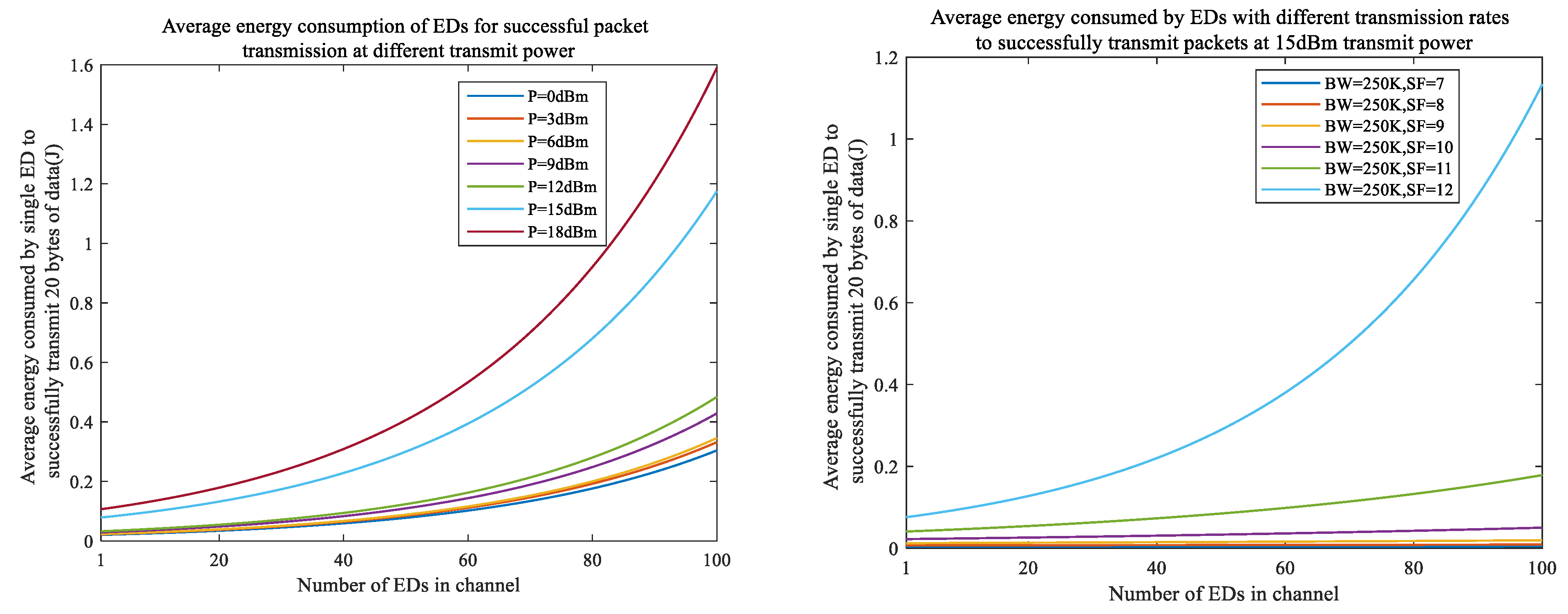
4.2. ED Throughput and the Power Consumption Model

The main purpose of the link parameter adaptation is to maximize the throughput and minimize the ED energy consumption while ensuring a sufficient link budget. The following is the model of the ED throughput and the energy consumption under the premise of link reachability.

4.2.1. ED Throughput Model under the Link Reachability

The gateway designed, based on the SX1278/SX1262 chip cannot achieve a single channel multi SF demodulation, such as the gateway designed, based on the SX1301 chip. The single channel parameters are a fixed design, and can only demodulate the packets sent by the EDs with the same link parameters. The following is the throughput model of the EDs in a single channel. Assuming that the packet generation process of each ED follows a Poisson process, with an average generation rate of $\lambda$ packets per second and a packet length of $L$ bytes and assuming that the number of channels is $i$, the number of EDs in the i-th channel is $N_i$, $G_i$ denotes the number of packets generated when transmitting packets in the i-th channel, and the probability of a successful transmission in the i-th channel under the pure ALOHA protocol is

$$P_{succ}=e^{-2G_i}$$

(6)

The probability of conflict is

$$P_{coll}=1-e^{-2G_i}$$

(7)

The time required to transmit the packets is

$$T_i=\frac{L}{R_b}$$

(8)

$L$ denotes the packet length, $R_b$ denotes the bit rate [2], and

$$R_b=SF\times \frac{BW}{2^{SF}}\times CR$$

(9)

The total traffic generated by the i-th channel per unit of time is:

$${\lambda }_i=\frac{N_i}{T_{span}}$$

(10)

$N_i$ denotes the number of i-th channel EDs and $T_{span}$ denotes the average time interval for each ED to generate packets.

Then, the traffic generated by the i-th channel in time $T_i$

$${\lambda }_i=\frac{N_i}{T_{span}}$$

(11)

Then, the conflict probability when a single ED sends a packet is

$$P_{coll,i}=1-e^{-2{\lambda }_i{T}_i}=1-e^{-\frac{{\lambda }_{i}L·2^{SF+1}}{SF·BW·CR}}$$

(12)

Then, the average throughput of a single ED in the i-th channel is

$$\mathsf{\Gamma }={\lambda }_{\mathrm{n}}\cdot L\cdot P_{succ,i}$$

(13)

${\lambda }_n$ indicates the number of packages generated by a single ED per unit of time.

Figure 10 shows the variation of a single ED throughput at different rates, as the number of EDs in the channel increases, the EDs in the channel generate one 20-byte packet every 20 s at different rates. It can be concluded that the lower the communication rate, the lower the network throughput, and the more the number of nodes in the channel, the channel conflict increases and the throughput decreases.

4.2.2. ED Energy Consumption Model

The total energy consumption is the sum of the sleep energy consumption $E_{sleep}$ and the active energy consumption $E_{active}$

$$E_{sum}=E_{sleep}+E_{active}$$

(14)

The ED transmits a data frame, and there are two cases: transmission failure (retransmission required) and successful transmission. Assuming that the probability of a successful transmission without conflict is $p$, the probability of failure is $1-p$, and follows a binomial distribution. The average energy consumption of successfully transmitting a data frame is

$$E_{avg}={\displaystyle \sum _{k=1}^{\infty }{(1-p)}^{k-1}p[(k-1)E_{failed}+E_{succ}]=\frac{1-p}{p}{E}_{failed}+E_{succ}}$$

(15)

$$E_{failed}=E_{TX}+E_{RXtimeout}$$

(16)

$$E_{succ}=E_{TX}+E_{RXack}$$

(17)

$$E_{succ}=Curr{[P]}_{send}\cdot V\cdot \frac{L_{payload}}{R_b}+Curr{[P]}_{recv}\cdot V\cdot \frac{L_{ack}}{R_b}$$

(18)

$E_{TX}$ indicates the energy consumed to send the data frame, $E_{RXtimeout}$ is the energy consumed by the unaccepted ACK, $E_{RXack}$ is the energy consumed by receiving ACK, $Curr[P]$ represents the operating current when the ED power is P, $R_b$ represents the data rate, $L$ represents the transmission packet length, $V$ indicates the node operating voltage, which is 3.3 V in the ED we are using.

The average energy consumed by the EDs to successfully transmit a packet is calculated as follows, $E$ represents the average energy consumption of EDs to successfully transmit a packet [22], n represents the number of nodes, PRR represents the average physical layer packet receipt rate [23].

$$E=\frac{\frac{{\displaystyle \sum _{i=1}^n{E}_{av{g}_i}}}{n}}{PR{R}_{avg}}$$

(19)

Figure 11 shows the average energy consumed by a single ED to successfully transmit a packet, as the number of EDs in the channel increases, under the different transmit power and rate conditions, and the EDs in the channel generate a 20-byte packet every 20 s.

4.3. Link Parameter Adaptation Algorithm

A single ED parameter adaptation problem can be transformed into an optimization problem with a guaranteed sufficient link budget to maximize the throughput and minimize the energy consumption [24,25,26,27]. The transmission parameter $S_i$ is composed of $(BW,SF,CR,N,TP)$, where $N$ indicates the number of EDs currently connected to the channel. $(BW,SF,CR)$ is selected among the gateway channels with fixed parameters, and the single ED parameter configuration problem is transformed into an optimization problem.

$$\begin{array}{c}\underset{s_i}{\max }\mathsf{\Gamma }\\ s.t.\{\begin{array}{l}\begin{array}{l}\begin{array}{l}{S}_i\in S\\ TP-PL\ge to{l}_{s_i}\end{array}\hfill \\ TP\in \left\{-4,-1,2,5,8,11,14\right\}\hfill \end{array}\hfill \\ \begin{array}{l}SF\in \{7,8,9,10,11,12\}\\ BW\in \{62.5,125,250,500\}\\ CR\in \{\frac{4}{5},\frac{4}{6},\frac{4}{7},\frac{4}{8}\}\end{array}\hfill \end{array}\end{array}$$

(20)

$to{l}_{s_i}$ indicates the sensitivity under the $S_i$ parameter [28,29], and if the throughput is equal, the set of parameters that minimizes the energy consumption of the ED transmission is considered

$$\begin{array}{c}\underset{s_i}{\min }{\mathrm{E}}_{avg}\\ s.t.\{\begin{array}{l}\begin{array}{l}\begin{array}{l}{S}_i\in S\\ TP-PL\ge to{l}_{s_i}\end{array}\hfill \\ TP\in \left\{-4,-1,2,5,8,11,14\right\}\hfill \end{array}\hfill \\ \begin{array}{l}SF\in \{7,8,9,10,11,12\}\\ BW\in \{62.5,125,250,500\}\\ CR\in \{\frac{4}{5},\frac{4}{6},\frac{4}{7},\frac{4}{8}\}\end{array}\hfill \end{array}\end{array}$$

(21)

In Section 3, the link quality was evaluated for different rates, and the different link adaptation strategies are required for the different evaluation results.

• Allocate a sufficient link budget

For the good link quality, it means that the PRR is greater than 90%. At this time, the data rate should be accelerated as far as possible on the premise of a sufficient link budget, which can reduce the ED energy consumption. When the rate is the fastest, the transmission power should be reduced. When the link budget is insufficient, it is not necessary to adjust the rate and the PRR should be stabilized to be greater than 90% to meet the application requirements, and avoid the huge overhead caused by the frequent adjustment of the data rate.

For a bad link quality, it means that the PRR is less than 90%. The measurement and classification results show that the link budget must be insufficient at this time, so it is necessary to increase the link budget. The first strategy is to increase the transmission power without reducing the data rate, because reducing the rate would result in a higher energy consumption due to the increased airtime, so only consider reducing the data rate when the transmission power is highest.

2.

Following the above adjustment, the minimum demodulation sensitivity that meets the current ED can be calculated.

3.

Finding the optimal channel parameters.

4.

In the previous step, the minimum sensitivity that satisfies the stable operation of the current ED is obtained. Traverse the currently available channels that satisfy the sensitivity conditions, and find the channel that exactly satisfies the demodulation sensitivity and maximizes the throughput of the current ED. If the throughput is the same, the channel with the minimum energy consumption of the ED is the optimal channel. Issue the configuration parameters.

Based on the previously obtained optimal channel, the link parameters of the optimal channel are configured into the current ED.

The designed link parameter adaptation method can be applied to the above-mentioned LoRa network with the SX1278/SX1262 gateways, and can also be applied to the LoRaWAN network with the SX1301 gateway [30,31]. The following are the link parameter adaptation algorithms designed for the two link qualities, respectively.

Table 4. Description of the algorithm parameters.

Algorithm Parameters	Parameter Description
$SN{R}_{avg}$$RSS{I}_{avg}$	Average value of the hardware parameters during the window
$M$	Link margin, default is 10 dBm
$Channel[:]$	List of channels sorted according to reception sensitivity
$SN{R}_{\min }$	Minimum demodulation signal-to-noise ratio
$P{t}_{sensitivity}$	Demodulation sensitivity

presents the algorithm parameters. The algorithm runs as Algorithms 1 and 2.

Algorithm 1: Good Link Quality Link Parameter Adaptation Algorithm

INPUT: $\begin{array}{l}S{F}_{temp}=S{F}_{cur},P{t}_{temp}=P{t}_{cur},B{W}_{temp}=B{W}_{cur},S{F}_{\min }=7,B{W}_{\max }=500k,B{W}_{\min }=62.5k\\ RSS{I}_{avg},SN{R}_{avg},SN{R}_{\min },P{t}_{sensitivity},Channel[:]\\ SN{R}_{m\arg in}=SN{R}_{avg}-SN{R}_{\min }-M\\ N_{step}=\left[\frac{SN{R}_{m\arg in}}{3}\right]\end{array}$ OUTPUT:$B{W}_{next},S{F}_{next},P{t}_{next}$

If $N_{step}>0$ then         while $N_{step}>0$ $\&$ $S{F}_{temp}>S{F}_{\min }$ $\&$ $RSS{I}_{avg}>P{t}_{sensitivity}-3dB$ do                $\begin{array}{l}S{F}_{temp}=S{F}_{temp}-1\\ P{t}_{sensitivity}=P{t}_{sensitivity}+3dB\\ N_{step}=N_{step}-1\end{array}$             If $RSS{I}_{avg}-P{t}_{sensitivity}<=M$ then               return $B{W}_{next}=B{W}_{temp},S{F}_{next}=S{F}_{temp},P{t}_{next}=P{t}_{temp}$         while $N_{step}>0$ $\&$ $B{W}_{temp}<B{W}_{\max }$ $\&$ $RSS{I}_{avg}>P{t}_{sensitivity}-3dB$ do              $\begin{array}{l}B{W}_{temp}=B{W}_{temp}+1\\ N_{step}=N_{step}-1\\ P{t}_{sensitivity}=P{t}_{sensitivity}+3dB\end{array}$             If $RSS{I}_{avg}-P{t}_{sensitivity}<=M$ then                return $B{W}_{next}=B{W}_{temp},S{F}_{next}=S{F}_{temp},P{t}_{next}=P{t}_{temp}$         while $N_{step}>0$ $\&$ $P{t}_{temp}<P{t}_{\max }$ do            $P{t}_{temp}=P{t}_{temp}-3dB$              $N_{step}=N_{step}-1$         $optimalIndex=0$         For $i=1$ to $Channel[:].size()$ do           If $Channel[i].P{t}_{senditivity}<=P{t}_{senditivity}$ $\&$ $Channel[i].SF>=S{F}_{temp}$ do                If ${\mathsf{\Gamma }}_i>{\mathsf{\Gamma }}_{optimalIndex}$ do               $optimalIndex=i$            Else if ${\mathsf{\Gamma }}_i={\mathsf{\Gamma }}_{optimalIndex}$ do                If $E_i<E_{optimalIndex}$ do                  $optimalIndex=i$ Return $B{W}_{next}=Channel[optimalIndex].BW,S{F}_{next}=Channel[optimalIndex].SF,P{t}_{next}=P{t}_{temp}$

Algorithm 2: Bad Link Quality Link Parameter Adaptation Algorithm

INPUT: $\begin{array}{l}S{F}_{temp}=S{F}_{cur},P{t}_{temp}=P{t}_{cur},B{W}_{temp}=B{W}_{cur},S{F}_{\max }=12,B{W}_{\max }=500k,B{W}_{\min }=62.5k\\ RSS{I}_{avg},SN{R}_{avg},SN{R}_{\min },P{t}_{sensitivity},Channel[:]\\ SN{R}_{m\arg in}=SN{R}_{avg}-SN{R}_{\min }-M\\ N_{step}=\left[\frac{SN{R}_{m\arg in}}{3}\right]\end{array}$ OUTPUT:$B{W}_{next},S{F}_{next},P{t}_{next}$

If$N_{step}<0$then     While $N_{step}<0$ $\&$ $P{t}_{temp}<P{t}_{\max }$ do           $P{t}_{temp}=P{t}_{temp}+3dB$           $N_{step}=N_{step}+1$           $P{t}_{sensitivity}=P{t}_{sensitivity}-3dB$ While $N_{step}<0$ $\&$ $B{W}_{temp}>B{W}_{\min }$ do           $\begin{array}{l}B{W}_{temp}=B{W}_{temp}-1\\ N_{step}=N_{step}+1\\ P{t}_{sensitivity}=P{t}_{sensitivity}-3dB\end{array}$          While $N_{step}<0$ $\&$ $S{F}_{temp}<S{F}_{\max }$ do          $\begin{array}{l}S{F}_{temp}=S{F}_{temp}+1\\ P{t}_{sensitivity}=P{t}_{sensitivity}-3dB\\ N_{step}=N_{step}+1\end{array}$     $optimalIndex=0$     For $i=1$ to $Channel[:].size()$ do         If $Channel[i].P{t}_{sensitivity}<=P{t}_{sensitivity}$ $\&$ $Channel[i].SF>=S{F}_{temp}$ do            If ${\mathsf{\Gamma }}_i>{\mathsf{\Gamma }}_{optimalIndex}$ do                $optimalIndex=i$            Else if ${\mathsf{\Gamma }}_i={\mathsf{\Gamma }}_{optimalIndex}$ do                If $E_i<E_{optimalIndex}$ do                  $optimalIndex=i$ Return $B{W}_{next}=Channel[optimalIndex].BW,S{F}_{next}=Channel[optimalIndex].SF,P{t}_{next}=P{t}_{temp}$

5. Testing and Result Analysis

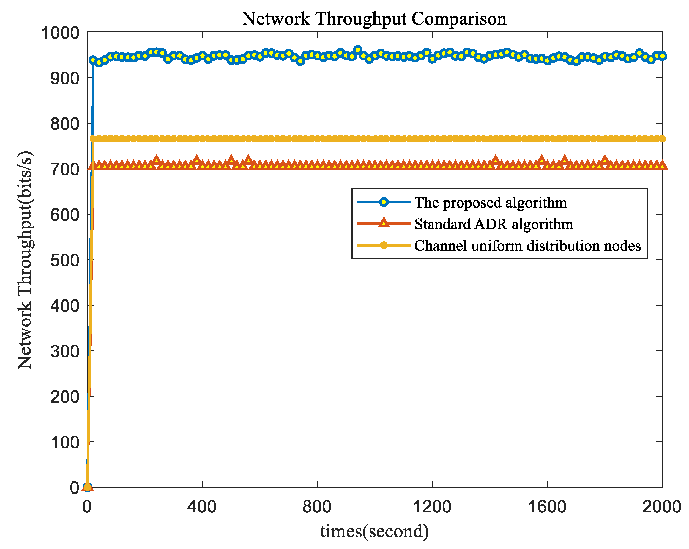
5.1. Single ED Scenario

As in Figure 4 and Figure 12, the gateway is deployed on the roof of a 20 m high building, the ED is 572 m from the gateway. The ED parameters were initially configured, as follows in

Table 5. Single ED initial parameter configuration.

Parameter	Value
BW	500 KHz
SF	7
Frequency	433 MHz
Packet length	20 Bytes
Transmit power	10 dBm
Preamble length	10
CR	4/5
Distance from the gateway	572 m
Packet generation rate	1 s
Height of the gateway	20 m

. The bandwidth is 500 k, the spreading factor is 7. The ED generates one packet per second, and the packets’ reception rate is calculated every 20 s. The PRR changes with 2000 s under the proposed algorithm, the standard ADR and the static parameter settings are compared.

Figure 13 shows the change of the PRR of the different algorithms. Following the final three methods are implemented, the parameters of the nodes are configured, as shown in

Table 6. Final parameter configuration for three methods.

Method	BW	SF	P
The proposed algorithm	250 KHz	8	10 dBm
LoRaWAN ADR	500 KHz	7	13 dBm
Static algorithm	500 KHz	7	10 dBm

. Figure 14 shows the comparison of the different algorithms. It can be concluded that the PRR of the proposed algorithm is improved by 27%, compared with the standard ADR, and 52% when compared with static parameters. The main reason is that the standard ADR uses the maximum SNR in the window period to evaluate the current channel, while, for the shadow fading channel, it tends to use a faster rate, resulting in a higher packet loss rate. The proposed algorithm first classifies the link quality, according to the hardware parameters. To ensure an accurate link quality evaluation, the link with the PRR lower than 90%, is classified as a bad link. To improve the link budget of the bad links, so that the link quality is stable in a good range, the PRR has to reach over 90%.

5.2. Multi-ED Scenario

Thirty-two EDs were evenly distributed at 100 m, 200 m, 300 m, 500 m, 700 m, 1 km, 1.5 km, and 2 km away from the gateway, The gateway is deployed on the 20-m-tall roof of the School of Communication and Information Engineering of Xi’an University of Posts and Telecommunications. The initial parameters of all of the EDs were the lowest rate, as shown in

Table 7. Muti-Eds’ initial parameter configuration.

Parameter	Value
BW	62.5 KHz
SF	12
Frequency	433 MHz
Packet length	20 Bytes
Transmit power	10 dBm
Preamble length	10
CR	10
Distance from the gateway	100 m, 200 m, 300 m, 500 m, 700 m, 1 Km, 1.5 Km, 2 Km
Packet generation rate	5 s
Number of EDs	32

. All EDs start working on channel 8 of the gateway, the BW was 62.5 KHz, the SF was 12, and the P was 10 dBm. The 8 channels were configured on the gateway side. The channel parameter settings are set, as shown in

Table 8. Gateway channel parameter configuration.

Gateway Channel No.	BW	SF	P
1	500 KHz	7	15 dBm
2	250 KHz	8	15 dBm
3	250 KHz	9	15 dBm
4	125 KHz	9	15 dBm
5	62.5 KHz	8	15 dBm
6	125 KHz	10	15 dBm
7	62.5 KHz	10	15 dBm
8	62.5 KHz	12	15 dBm

. Figure 15 shows the initial location distribution of the 32 EDs, the starting parameters of all of the nodes are located on channel 8 of the gateway, as shown in Table 7. Figure 16 shows the actual deployment environment. When the algorithm is running, the parameters of the nodes are changed and will be adjusted to each channel of the gateway. A 20-byte packet is generated every 5 s, and the network throughput is calculated every 20 s. The proposed algorithm counts the network throughput variation within 2000 s, and is compared with the standard ADR algorithm and the channel uniform distribution ED algorithm.

Figure 17 shows the final number of EDs per channel of the gateway after the algorithm execution is completed after 2000 s, and the final number of EDs for channel 1 is 14. This is because channel 1 has the fastest rate and the corresponding smaller conflict probability, the more EDs can be accommodated, and it can be seen that the proposed algorithm tries to adjust the EDs to the channel with a small conflict probability under the premise of ensuring a link reliability, which ensures the link reliability and the network throughput. Figure 18 shows the variation of the whole network throughput for different algorithms during the 2000 s. The throughput of the proposed algorithm is 34.12% higher than that of the standard ADR and 24.14% higher than that of the algorithm that divides the EDs into different channels, equally. This is mainly because the proposed algorithm first classifies the link quality, allocates the different link adaptation algorithms according to the different link qualities, and ensures the highest throughput of the ED on the premise of ensuring a sufficient link budget. Since the LoRaWAN ADR uses the SX1301 chip, it only supports a 125 KHz bandwidth, so only the SF and the power can be adjusted. The LoRaWAN ADR without a fixed channel limit, tends to be faster and consumes less energy, but the resulting packet loss is also more obvious. The proposed algorithm is applied to the SX1278/SX1262 gateway, which supports the multi-channel low-bandwidth, but does not support the single-channel multi-SF demodulation. On the premise of ensuring the link stability, the channel with the highest throughput is used to ensure a low packet loss rate.

Figure 19 shows the average energy consumption of all EDs for the successful transmission of a packet calculated, as in Equation (19), and the average packet reception rate of the two algorithms for the 32 EDs, the final parameters of the 32 EDs are configured in Figure 17, and the rate is the rate of the channel where they are located. It can be seen that the packet reception rate is 26% higher than that of the LoRaWAN ADR, while the average energy consumption of the EDs for the successful transmission of a packet is slightly lower than that of the LoRaWAN ADR. The proposed algorithm can significantly improve the packet reception rate and ensure the stability of the link. Because the LoRaWAN ADR adopts a more aggressive strategy to adjust the rate [15,32], it tends to adopt a faster rate which leads to a more serious packet loss and does not consider the MAC layer conflict [33]. Although a faster rate means a lower energy consumption of the ED, the physical layer packet loss and the MAC layer conflict will bring the packet retransmission, resulting in more energy consumption to actually transmit a packet successfully [34]. If the energy consumption is calculated without considering the MAC layer conflict and the physical layer packet loss, the LoRaWAN ADR consumes less energy. Figure 20 shows the comparison of the energy efficiency of the two algorithms calculated [22], as in Equation (22), L represents a package length which is 160 bits, and E is calculated, as in Equation (19), and it can be seen that the energy efficiency of the two algorithms is essentially equal. However, the proposed algorithm is able to bring a significant improvement in the throughput and the PRR.

$${\eta }_{EE}=\frac{L}{E}$$

(22)

5.3. Algorithm Complexity Analysis

On a normal 2.4 GHz CPU main frequency and 8 GB memory server, the algorithm execution time is divided into two parts. one part is based on the link quality classification of the previously trained support vector machine model, and the time used for a single classification is 0.000322 ms. The other part is the link parameter adaptation, the algorithm complexity is O(n). The algorithm execution time for a single execution under the condition of 1000 channels is 0.7669 ms, and the total running time is 0.767 ms, which can meet the requirements of the application.

6. Conclusions

In this paper, an adaptive rate algorithm is proposed for the practically deployed low-cost LoRa gateways. Firstly, the link quality is classified, based on the fuzzy support vector machine, secondly, the different link parameter adaptation algorithms are designed, based on the different link qualities, considering both the link-level performance and the MAC layer performance, and finally, the proposed algorithm is verified in a practically deployed LoRa network. The experimental results show that the PRR of the proposed algorithm can be stabilized above 90% for a single link, which is 27% higher than the standard LoRaWAN ADR. For multiple EDs, with a packet generation rate of 5 s per ED and a packet length of 20 Bytes, the proposed algorithm achieves an average PRR of 97%, and the throughput is improved by 34.12%, compared with the standard ADR. Therefore, the throughput and the PRR of the LoRa network can be significantly improved with a comparable energy consumption and the LoRaWAN ADR, which verifies the effectiveness of the proposed algorithm. However, the proposed algorithm still has some limitations. On the one hand, the algorithm has a high computational complexity and cannot be deployed in some edge devices with insufficient computing power, and on the other hand, the algorithm does not consider the heterogeneity of the network, and most IoT networks in practice have heterogeneous characteristics. The future improvement of the algorithm can start from the above two directions.

References

1. Kufakunesu, R.; Hancke, G.; Abu-Mahfouz, A. A Survey on Adaptive Data Rate Optimization in LoRaWAN: Recent Solutions and Major Challenges. Sensors 2020, 20, 5044. [Google Scholar] [CrossRef] [PubMed]
2. SemtechCorporation. LoRa Modulation Basics. 2015. Available online: http://wiki.lahoud.fr/lib/exe/fetch.php?media=an1200.22.pdf (accessed on 29 August 2022).
3. Benkahla, N.; Tounsi, H.; Song, Y.Q.; Frikha, M. Review and experimental evaluation of ADR enhancements for LoRaWAN networks. Telecommun. Syst. 2021, 77, 1–22. [Google Scholar] [CrossRef]
4. Almuhaya, M.A.M.; Jabbar, W.A.; Sulaiman, N.; Abdulmalek, S. A Survey on LoRaWAN Technology: Recent Trends, Opportunities, Simulation Tools and Future Directions. Electronics 2022, 11, 164. [Google Scholar] [CrossRef]
5. Arshad, J.; Aziz, M.; Al-Huqail, A.A.; Zaman, M.H.u.; Husnain, M.; Rehman, A.U.; Shafiq, M. Implementation of a LoRaWAN Based Smart Agriculture Decision Support System for Optimum Crop Yield. Sustainability 2022, 14, 827. [Google Scholar] [CrossRef]
6. Jabbar, W.A.; Subramaniam, T.; Ong, A.E.; Shu’Ib, M.I.; Wu, W.; de Oliveira, M.A. LoRaWAN-Based IoT System Implementation for Long-Range Outdoor Air Quality Monitoring. Internet Things 2022, 19, 100540. [Google Scholar] [CrossRef]
7. Lodhi, M.; Wang, L.; Farhad, A. ND-ADR: Nondestructive adaptive data rate for LoRaWAN Internet of Things. Int. J. Commun. Syst. 2022, 35, e5136. [Google Scholar] [CrossRef]
8. Almuhaya, M.A.M.; Jabbar, W.A.; Sulaiman, N.; Sulaiman, A.H.A. An Overview on LoRaWAN Technology Simulation Tools. In Proceedings of the Advances on Intelligent Informatics and Computing; Saeed, F., Mohammed, F., Ghaleb, F., Eds.; Springer International Publishing: Cham, Germany, 2022; pp. 345–358. [Google Scholar]
9. He, T.; Ren, Q.; Chen, D. Analysis of Node Performance in LoRaWAN Network Based on Markov Chain. Chin. J. Sens. Actuators 2018, 31, 1399–1405. [Google Scholar]
10. Zacharias, S.; Newe, T.; O’Keeffe, S.; Lewis, E. 2.4 GHz IEEE 802.15.4 channel interference classification algorithm running live on a sensor node. In Proceedings of the SENSORS, Taipei, Taiwan, 28–31 October 2012; IEEE: Piscataway Township, NJ, USA, 2012; pp. 1–4. [Google Scholar]
11. Wang, H.; Jia, J. Research on Data-Driven LoRa Link Quality Estimation. In Proceedings of the 2024 4rd International Conference on Natural Language Processing (ICNLP), Guangzhou, China, 24–26 March 2022; pp. 9–13. [Google Scholar]
12. Dong-xu, F.; Dong-qin, F.; He-nan, Z. Mean LQI and RSSI based link evaluation algorithm and the application in frequency hopping mechanism in wireless sensor networks. In Proceedings of the 2011 International Conference on Consumer Electronics, Communications and Networks (CECNet), Xianning, China, 16–18 April 2011; pp. 3252–3257. [Google Scholar]
13. De, D.; Daniel, C.; John, A.; Morris, B. A High-Throughput Path Metric for Multi-Hop Wireless Routing. Wirel. Netw. 2003, 11, 134–146. [Google Scholar]
14. Liu, L.; Xiao, T.; Xia, Y. Link Quality Estimation Based on Extremely Fast Decision Tree. J. Beijing Univ. Posts Telecommun. 2021, 44, 125–130. [Google Scholar]
15. SemtechCorporation. LoRaWAN—Simple Rate Adaptation Recommended Algorithm. 2016. Available online: https://www.thethingsnetwork.org/forum/uploads/default/original/2X/7/7480e044aa93a54a910dab8ef0adfb5f515d14a1.pdf (accessed on 29 August 2022).
16. Cai, Q.; Lin, J.; Xia, C. Adaptive Configuration Strategy on LoRa Networks for Multi-Heterogeneous IoT Applications. Comput. Syst. Appl. Chin. 2020, 29, 1–10. [Google Scholar]
17. Marini, R.; Cerroni, W.; Buratti, C. A Novel Collision-Aware Adaptive Data Rate Algorithm for LoRaWAN Networks. IEEE Internet Things J. 2021, 8, 2670–2680. [Google Scholar] [CrossRef]
18. Abdelfadeel, K.Q.; Cionca, V.; Pesch, D. Fair Adaptive Data Rate Allocation and Power Control in LoRaWAN. In Proceedings of the 2018 IEEE 19th International Symposium on ”A World of Wireless, Mobile and Multimedia Networks” (WoWMoM), Chania, Greece, 12–15 June 2018; pp. 14–15. [Google Scholar]
19. Sandoval, R.M.; Garcia-Sanchez, A.J.; Garcia-Haro, J. Optimizing and Updating LoRa Communication Parameters: A Machine Learning Approach. IEEE Trans. Netw. Serv. Manag. 2019, 16, 884–895. [Google Scholar] [CrossRef]
20. Luo, X.; Liu, L.; Shu, J.; AlKali, M. Link Quality Estimation Method for Wireless Sensor Networks Based on Stacked Autoencoder. IEEE Access 2019, 7, 21572–21583. [Google Scholar] [CrossRef]
21. Reynders, B.; Meert, W.; Pollin, S. Power and spreading factor control in low power wide area networks. In Proceedings of the 2017 IEEE International Conference on Communications (ICC), Paris, France, 21–25 May 2017; pp. 1–6. [Google Scholar]
22. Li, Y.; Yang, J.; Wang, J. DyLoRa: Towards Energy Efficient Dynamic LoRa Transmission Control. In Proceedings of the IEEE INFOCOM 2020—IEEE Conference on Computer Communications, Toronto, ON, Canada, 6–9 July 2020; pp. 2312–2320. [Google Scholar]
23. Premsankar, G.; Ghaddar, B.; Slabicki, M.; Francesco, M.D. Optimal Configuration of LoRa Networks in Smart Cities. IEEE Trans. Ind. Inform. 2020, 16, 7243–7254. [Google Scholar] [CrossRef]
24. Amichi, L.; Kaneko, M.; Fukuda, E.H.; El Rachkidy, N.; Guitton, A. Joint Allocation Strategies of Power and Spreading Factors With Imperfect Orthogonality in LoRa Networks. IEEE Trans. Commun. 2020, 68, 3750–3765. [Google Scholar] [CrossRef] [Green Version]
25. Sandoval, R.M.; Rodenas-Herraiz, D.; Garcia-Sanchez, A.J.; GarciaHaro, J. Deriving and Updating Optimal Transmission Configurations for Lora Networks. IEEE Access 2020, 8, 38586–38595. [Google Scholar] [CrossRef]
26. Reynders, B.; Wang, Q.; Tuset-Peiro, P.; Vilajosana, X.; Pollin, S. Improving Reliability and Scalability of LoRaWANs Through Lightweight Scheduling. IEEE Internet Things J. 2018, 5, 1830–1842. [Google Scholar] [CrossRef]
27. Finnegan, J.; Farrell, R.; Brown, S. Analysis and Enhancement of the LoRaWAN Adaptive Data Rate Scheme. IEEE Internet Things J. 2020, 7, 7171–7180. [Google Scholar] [CrossRef]
28. Hoeller, A.; Souza, R.D.; Montejo-S’anchez, S.; Alves, H. Performance Analysis of Single-Cell Adaptive Data Rate-Enabled LoRaWAN. IEEE Wirel. Commun. Lett. 2020, 9, 911–914. [Google Scholar] [CrossRef] [Green Version]
29. El-Aasser, M.; Elshabrawy, T.; Ashour, M. Joint Spreading Factor and Coding Rate Assignment in LoRaWAN Networks. In Proceedings of the 2018 IEEE Global Conference on Internet of Things (GCIoT), Alexandria, Egypt, 5–7 December 2018; pp. 1–7. [Google Scholar]
30. Yao, Y.; Chen, X.; Rao, L.; Liu, X.; Zhou, X. LORA: Loss Differentiation Rate Adaptation Scheme for Vehicle-to-Vehicle Safety Communications. IEEE Trans. Veh. Technol. 2017, 66, 2499–2512. [Google Scholar] [CrossRef]
31. Liao, W.S.; Zhao, O.; Ishizu, K.; Kojima, F. Adaptive Parameter Adjustment for Uplink Transmission for Multi-gateway LoRa Systems. In Proceedings of the 2019 22nd International Symposium on Wireless Personal Multimedia Communications (WPMC), Lisbon, Portugal, 24–27 November 2019; pp. 1–5. [Google Scholar]
32. Ksiazek, K.; Grochla, K. Flexibility Analysis of Adaptive Data Rate Algorithm in LoRa Networks. In Proceedings of the 2021 International Wireless Communications and Mobile Computing (IWCMC), Harbin, China, 28 June–2 July 2021; pp. 1393–1398. [Google Scholar]
33. Heeger, D.; Garigan, M.; Plusquellic, J. Adaptive Data Rate Techniques for Energy Constrained Ad Hoc LoRa Networks. In Proceedings of the 2020 Global Internet of Things Summit (GIoTS), Dublin, Ireland, 3–5 June 2020; pp. 1–6. [Google Scholar]
34. Adi, P.D.P.; Kitagawa, A. Performance Evaluation of Low Power Wide Area (LPWA) LoRa 920 MHz Sensor Node to Medical Monitoring IoT Based. In Proceedings of the 2020 10th Electrical Power, Electronics, Communications, Controls and Informatics Seminar (EECCIS), Malang, Indonesia, 26–28 August 2020; pp. 278–283. [Google Scholar]
Figure 1. Fitting diagram of the SNR and PRR.
Mathematics 10 03920 g001
Figure 2. Fitting diagram of the RSSI and PRR.
Mathematics 10 03920 g002
Figure 3. Link quality of the division diagram.
Mathematics 10 03920 g003
Figure 4. Outdoor test scenario. (a) The actual deployment location of the gateway; (b) Packet collection scenario.
Mathematics 10 03920 g004
Figure 5. Link quality classification under BW = 62.5 KHz, SF = 12.
Mathematics 10 03920 g005
Figure 6. Link quality classification under BW = 500 Khz, SF = 7.
Mathematics 10 03920 g006
Figure 7. The optimization process of the model parameters is under BW = 500 khz SF = 12. (a) Optimal C solving; (b) Optimal b solving.
Mathematics 10 03920 g007
Figure 8. Gateway hardware design.
Mathematics 10 03920 g008
Figure 9. ED hardware design.
Mathematics 10 03920 g009
Figure 10. The channel throughput changes with the increase of the number of EDs in the channel.
Mathematics 10 03920 g010
Figure 11. As the number of EDs in the channel increases, the energy consumed by an ED to successfully transmit a frame changes.
Mathematics 10 03920 g011
Figure 12. Experimental scenario 1.
Mathematics 10 03920 g012
Figure 13. PRR variation for the different algorithms on a single link.
Mathematics 10 03920 g013
Figure 14. Algorithm comparison.
Mathematics 10 03920 g014
Figure 15. Multi-ED location distribution.
Mathematics 10 03920 g015
Figure 16. ED and gateway deployment locations.
Mathematics 10 03920 g016
Figure 17. Number of the different channel EDs after the rate adjustment by the proposed algorithm.
Mathematics 10 03920 g017
Figure 18. Throughput comparison of the different algorithms.
Mathematics 10 03920 g018
Figure 19. Comparison of the different algorithms.
Mathematics 10 03920 g019
Figure 20. Energy efficiency comparison.
Mathematics 10 03920 g020