Bearing Fault Diagnosis Based on Discriminant Analysis Using Multi-View Learning

Abstract

Bearing fault diagnosis has been a challenge in rotating machinery and has gained considerable attention. In order to correctly classify faults, the conventional fault diagnosis methods are mostly based on vibration signals. However, features extracted from a single view of vibration signals may leave out useful information, which can cause the incompleteness of intrinsic information and increase the risk of the performance degradation of fault classifications. In this paper, a novel bearing fault diagnosis method, discriminant analysis using multi-view learning (DAML), is proposed to tackle this issue. Multi-view datasets referring to vibration and acoustic signals are obtained by carrying out a fast Fourier transform (FFT). Then, multi-view feature (MVF) representation, including view-invariant and category discriminative information in a common subspace, is achieved based on canonical correlation analysis (CCA) and uncorrelated linear discriminant analysis (ULDA). Ultimately, with the help of the K-nearest neighbor (KNN) classifier built on the multi-view features, bearing faults are identified. The extensive experimental results show that DAML can identify the bearing fault accurately and outperforms other competitive approaches.

1. Introduction

As indispensable mechanical components, bearings play an exceptionally vital role in almost all kinds of rotating machinery [1,2]. Owing to harsh operating conditions, bearings are prone to faults, which can lead to unscheduled downtime and unpredicted productivity losses for production facilities or even catastrophic consequence for mission-critical equipment or human casualties [3,4,5]. Therefore, it is essential to diagnose the bearings, aiming to prevent the occurrence of accidents, an issue that has gained increasing and considerable attention.

Due to the rotating nature of the measured signals from defective bearings, the periodic or quasi-periodic transient components often reflect important physical information related to the bearing fault dynamics [6,7]. Since the rich fault information of the equipment status is carried by the vibration signals, the use of vibration signals for fault detection is a reasonable choice and a set of features are extracted in order to classify the faults [8,9]. These features could be in the time domain, frequency domain, or time-frequency domain [10,11], such as the peak amplitude, skewness, kurtosis, Fourier spectrum, envelope spectrum, spectral kurtosis, and so on [11,12,13]. Samanta et al. [14] utilized time-domain features to characterize the bearing conditions and employed ANNs and SVM to diagnose bearing faults. Li et al. [15] extracted features from noise-contaminated vibration signals based on local mean decomposition and a multi-scale permutation entropy, and then realized fault identification via an improved support vector machine-based binary tree. In addition to vibration signals, the use of information concealed within acoustic signals has gained more and more attention in order to guarantee the safe operation of bearings [16,17]. With regard to feature extraction, Al-Ghamd et al. [18] reported that acoustic signals achieved early fault detection and provided an indication of the size of the artificially made defect. Ref. [19] compared the use of vibration on a bearing run at 1440 rpm, and it was clear that the acoustic signal peak amplitude performed a more reliable detection of the bearing defect than the RMS of the vibration signal. In another study [20], the acoustic signal was more sensitive in tracking the progression of the defect than the vibration-based method. With regard to fault classification, Zhang et al. [21] applied a deep graph convolutional network based on graph theory for the acoustic-based fault diagnosis of roller bearings, which improved the fault classification accuracy.

Although many of the aforementioned works achieved successful applications in machine fault diagnosis, the features extracted were rarely described by the specific type of fault signal such as vibration signals or acoustic signals, which restricted the diagnostic accuracy and stability [22]. Both the measured vibration and acoustic signals are prone to being affected by background noise to varying degrees, and the collected vibration signals often have information loss [23,24]. Of course, feature refining of the vibration or acoustic signals can be carried out for performance enhancement. However, it is a time-consuming and unreliable type of human analysis.

As a matter of fact, the vibration and acoustic signals of the equipment are complementary and mutually enhanced [25]. In order to improve fault diagnosis performance, we could effectively utilize the information relevant to the equipment status stemming from the vibration and acoustic signals and enhance robustness. Some studies have been conducted that investigated the use of information fusion for fault diagnosis. In [26], a novel fault identification method using a correlation coefficient and Hurst exponent was proposed for depicting the actual fault mode from the decomposed signals, and the fault characteristics of rolling bearings were extracted. Shi et al. [25] proposed a two-stage sound-vibration signal-fusion algorithm, which enriched the fault characteristics’ information and improved signal-to-noise ratios significantly. Fei et al. [22] constructed the multi-feature entropy distance with vibration and acoustic signals, which reflected the process feature of rolling bearing faults with the change in the rotating speed, and the method had high diagnostic precision and strong robustness. However, these methods require extensive domain expertise, which is time-consuming and expensive. To automatically identify faults, methods based on machine learning have been developed for bearing feature analysis and fault diagnosis. In [27], a bearing fault diagnosis method based on a convolutional neural network using vibration and acoustic signals was presented and it could diagnose computer numerical control machine faults early. Wang et al. [28] proposed 1D-CNN-based networks for fusing vibration signals and acoustic signals, and the fault characteristics extracted from it could realize the accurate diagnosis of bearings. In another study [29], a deep random forest fusion technique using vibration and acoustic signals was used to improve fault diagnosis performance. However, these methods often need a large number of training samples to build models for fault diagnosis. In real-world scenarios, training samples are difficult to obtain and require extensive manual effort to label.

Recently, there has been a growing interest in multi-view learning as one type of research of information fusion, which aims to learn one function to model each view and jointly optimizes all the functions to improve the generalization performance and in addition, it provides the possibility of solving the above problem [30,31,32]. In [33], a discriminant common space was obtained by jointly learning multiple view-specific linear transforms for robust image recognition from multiple views. Yang et al. [34] proposed a novel discriminative regression-based framework that mapped the multi-view data to a unified low-dimensional discriminative subspace, which was further enhanced to be more discriminative for image classification. For image recognition under the condition of incomplete views, Zhang et al. [35] designed a cross-partial multi-view network that could fully and flexibly take advantage of multiple partial views and achieve competitive performance, especially under the condition of missing views. Wang et al. [36] designed and built a generative partial multi-view clustering model with adaptive fusion and cycle consistency to solve the incomplete multi-view problem by explicitly generating the data of missing views. Although many successes have been achieved in the classification of images, they have seldom been applied to fault detection and the diagnosis of rotating machinery components in industrial applications and they cannot be used without considering the characteristics of the signals. Furthermore, the extracted features can contain redundant or irrelevant information, which can reduce the fault diagnosis accuracy. Therefore, there is still broad room for improvement to realize an effective and high-accuracy fault diagnosis for actual scenarios.

In this paper, a novel bearing fault diagnosis method is proposed based on discriminant analysis using multi-view learning (DAML). First, multi-view datasets of normal bearings and faulty bearings from vibration and acoustic signals are obtained using a fast Fourier transform (FFT). Then, in order to achieve the robust feature representation for the different views, view-invariant and category discriminative multi-view features (MVF) are extracted by jointly seeking the most relevant relationships and optimal discriminant features with minimum redundancy in a common subspace based on canonical correlation analysis (CCA) and uncorrelated linear discriminant analysis (ULDA). Finally, with the help of a K-nearest neighbor (KNN) classifier built into the MVF, bearing faults are accurately identified. The main contribution of this work is the construction of view-invariant and category discriminative features via max-relevance and min-redundancy, and the features extracted from a small number of training samples can be successfully used for diagnosis.

The rest of this paper is organized as follows. Section 2 discusses the previous works and preliminaries including canonical correlation analysis and uncorrelated linear discriminant analysis. Section 3 introduces the fault diagnosis method based on discriminant analysis using multi-view learning, including multi-view feature dataset construction and multi-view feature extraction and diagnosis. Section 4 presents the experimental evaluations. The conclusions are given in Section 5.

2. Previous Works and Preliminaries

2.1. Canonical Correlation Analysis

Canonical correlation analysis (CCA) is an approach used for finding the common space in which the low dimensional embedding of features from two views are most correlated [33,37]. In other words, CCA learns a pair of transformations, one for each feature view, to, respectively, project the features to a common space. Both transformations were obtained by maximizing the cross correlation between the two feature views. To be specific, let $X_V=[x_{v_1},x_{v_2},\cdots ,x_{v_n}]\in R^{p\times n}$ and $X_A=[x_{a_1},x_{a_2},\cdots ,x_{a_n}]\in R^{q\times n}$ be the training samples from the vibration and acoustic signals, respectively, where $x_{v_i}\in R^{p\times 1},i=1,2,\cdots ,n$ denotes the sample from the vibration signals and $x_{a_i}\in R^{q\times 1},i=1,2,\cdots ,n$ denotes the sample from the acoustic signals. The two projection vectors, $w_v$ and $w_a$, can be described by the following problem:

$$arg\underset{w_v,w_a}{max}\frac{w_v^T{\mathsf{\Sigma }}_{va}{w}_a}{\sqrt{\left(w_v^T{\mathsf{\Sigma }}_{vv}{w}_v\right)\left(w_a^T{\mathsf{\Sigma }}_{aa}{w}_a\right)}}$$

(1)

where ${\mathsf{\Sigma }}_{va}$, ${\mathsf{\Sigma }}_{vv}$, and ${\mathsf{\Sigma }}_{aa}$ are the covariance matrices, which are calculated as

$$\left\{\begin{array}{c}{\mathsf{\Sigma }}_{va}=X_{V}H{X}_A^T\hfill \\ {\mathsf{\Sigma }}_{vv}=X_{V}H{X}_V^T\hfill \\ {\mathsf{\Sigma }}_{aa}=X_{A}H{X}_A^T\hfill \end{array}\right.$$

(2)

where $H=I-\frac{1}{n}l{l}^T$ and I is considered as l as the one vector. Since the objective is invariant to the scaling of $w_v$ and $w_a$, the projections are constrained to have unit variance and the above circumstance is equivalent to the following optimization problem:

$$arg\underset{w_v,w_a}{max}{w}_v^T{\mathsf{\Sigma }}_{va}{w}_{a}subjectto{w}_v^T{\mathsf{\Sigma }}_{vv}{w}_v=1,w_a^T{\mathsf{\Sigma }}_{aa}{w}_a=1$$

(3)

2.2. Uncorrelated Linear Discriminant Analysis

Uncorrelated linear discriminant analysis (ULDA) is an extension of linear discriminant analysis (LDA) and is an effective supervised feature extraction technique for maximum class separation and original class information maintenance in a single-view [38,39]. LDA seeks an orientation w to map the data into a subspace so that the ratio of the between-class distance to the within-class distance is maximized. Considering a multi-class pattern classification problem, we use $X=[X_1,X_2,\cdots ,X_c]$, which is partitioned into c classes, where $X_i\in R^{p\times n_i}$ and $n_i$ represent the size of the i-th class. Then, criteria are used to formulate the class separability in LDA, that is, the within-class scatter matrix $S_w$ and the between-class scatter matrix $S_b$, which are defined as

$$S_w=\sum _{i=1}^c\sum _{x_j\in X_i}(x_j-{\mu }_i){(x_j-{\mu }_i)}^T$$

(4)

$$S_b=\sum _{i=1}^c{n}_i({\mu }_i-\mu ){({\mu }_i-\mu )}^T$$

(5)

where ${\mu }_i$ denotes the mean of the samples in class i and $\mu$ denotes the mean of all samples. The optimal projection can be obtained by maximizing the Fisher criterion function, which is defined as

$$F\left(w\right)=\frac{w^T{S}_{b}w}{w^T{S}_{t}w}$$

(6)

In order to obtain the uncorrelated discriminant features, the jth direction $w_j$ is subjected to the following conjugated orthogonality constraints:

$$w_j^T{S}_t{w}_i$$

(7)

where $w_i(i=1,2,\cdots ,j-1)$ are the Fisher’s vectors and $S_t=S_w+S_b$ denotes the total scatter matrix. Then, the optimization problem can be transformed into the following form:

$$\begin{array}{cc}\hfill & \underset{w_j}{max}{w}_j^T{S}_{b}wj\hfill \\ \hfill & subjectto{w}_j^T{S}_t{w}_j=1,\hfill \\ \hfill & w_j^T{S}_t{w}_i=0,(i=1,2,\cdots ,j-1)\hfill \end{array}$$

(8)

Finally, $w_j$ of ULDA can be found successively via solving the following generalized eigenvalue problem [40]:

$$P_j{S}_b{w}_j={\lambda }_j{S}_w{w}_j$$

(9)

where

$$\begin{array}{cc}\hfill & P_1=I_p\hfill \\ \hfill & P_j=I_p-S_t{D}_j^T{\left(D_j{S}_t{S}_w^{-}1S_t{D}_j^T\right)}^{-}1D_j{S}_t{S}_w^{-}1(j>1)\hfill \\ \hfill & D_j={[w_1,w_2,\cdots ,w_{j-1}]}^T(j>1)\hfill \\ \hfill & I_p=diag(1,1,\cdots ,1)\in R^{p\times p}\hfill \end{array}$$

(10)

3. Fault Diagnosis Method Based on Discriminant Analysis Using Multi-View Learning

As mentioned in Section 1, learning from a single view may be non-robust and can lead to some uncertainty and incompleteness in the field of fault diagnosis. In order to solve this issue, we need to effectively utilize the information stemming from the multi-view datasets and capture more robust features for the training and test data. In this section, we present a novel bearing fault diagnosis method based on discriminant analysis using multi-view learning. The framework for this procedure is illustrated in Figure 1. The details of each part are elaborated in the following subsections.

3.1. Multi-View Feature Dataset Construction

If a bearing has a localized fault on the outer race, inner race, or a rolling element, during a constant speed operation, the fault point strikes the mating components and generates periodical impacts, which can be contained in the vibration and acoustic signals and, in general, these pieces of fault information can be identified in the frequency domain [3]. Hence, the impulsive features in the frequency domains of these two kinds of signals are the ideal candidates for monitoring and diagnosing.

In our work, raw time series signals and acoustic signals were acquired simultaneously and FFT amplitudes were caught, respectively, from them in the same time period, which guaranteed that the running state of the bearing could be represented from different views at the same time. Thus, the number of samples obtained from the vibration signals was equal to the number of samples obtained from the acoustic signals. The main steps of the multi-view dataset generation were as follows:

• Step 1: Catch the fixed-point FFT amplitudes from the raw time-series vibration and acoustic signals as samples $D_v\in R^{p\times n_v}$ and $D_a\in R^{q\times n_a}$, where $D_v$ denotes the vibration dataset and $D_a$ denotes the acoustic dataset. $n_v$ and $n_a$ represent the number of samples and p and q mean the dimensionality of the samples. In our work, p is equal to q.
• Step 2: Draw $X_{vtr}\in R^{p\times n_{vtr}}$ with label $Y_{vtr}\in R^{1\times n_{vtr}}$ from $D_v$ as the vibration training dataset randomly, where $n_{vtr}$ denotes the number of vibration training datasets. The remaining samples from $D_v$ are the vibration test dataset $X_{vte}\in R^{p\times n_{vte}}$.
• Step 3: Select $X_{atr}\in R^{q\times n_{atr}}$ with label $Y_{atr}\in R^{1\times n_{atr}}$ from $D_a$ as the acoustic training dataset randomly, where $n_{atr}$ denotes the number of acoustic training datasets. The remaining samples from $D_a$ are the acoustic test dataset $X_{ate}\in R^{q\times n_{ate}}$. Then, $X_{mtr}=[X_{vtr},X_{atr}]$, $Y_{mtr}=[Y_{vtr},Y_{atr}]$ and $X_{mte}=[X_{vte},X_{ate}]$ constitutes the multi-view feature dataset, referring to the vibration and acoustic views.

3.2. Multi-View Feature Extraction and Diagnosis

Although the view-invariant properties of the vibration and acoustic signals could be obtained in the common feature space using CCA, the discriminant information referring to the class structure properties was not explicitly taken into account, which created a risk of confusion in the classification. Thus, discriminant analysis was embedded for preserving the category discriminative properties in the process of further feature extraction. Accordingly, CCA and ULDA were applied for simultaneous view-invariant and category discriminative embedding. Therefore, the optimization problem of the multi-view feature extraction in this paper comprised Equations (3) and (8):

$$\begin{array}{cc}\hfill & \underset{w_{vr},w_{ar}}{max}(1-k)w_{vr}^T{S}_{bv}{w}_{vr}+k{w}_{ar}^T{S}_{ba}{w}_{ar}+2\gamma w_{vr}^T{\mathsf{\Sigma }}_{va}{w}_{ar}\hfill \\ \hfill & subjectto{w}_{vr}^T{S}_{tv}{w}_{vr}+\sigma w_{ar}^T{S}_{ta}{w}_{ar}=1,\hfill \\ \hfill & w_{vr}^T{S}_{tv}{w}_{vj}=w_{ar}^T{S}_{ta}{w}_{aj}=0,(j=1,2,\cdots ,r-1)\hfill \end{array}$$

(11)

where $w_{vr}$ and $w_{ar}$ represent the rth discriminant projection of $X_{vtr}$ and $X_{atr}$, respectively. k and $\gamma$ refer to the view-invariance and category discrimination. ${\mathsf{\Sigma }}_{va}$ denotes the covariance matrix, which can be acquired by

$${\mathsf{\Sigma }}_{va}=X_{vtr}H{X}_{atr}^T$$

(12)

$\sigma =$tr($S_{tv}$)/tr($S_{ta}$) guarantees that the optimization problem obtains a closed-form solution, where tr(·) denotes the trace of a matrix. $S_{bv}$ and $S_{ba}$ represent the between-class scatter matrix of the vibration training dataset $X_{vtr}$ and the acoustic training dataset $X_{atr}$, respectively. $S_{tv}$ and $S_{ta}$ represent the total scatter matrix of the vibration training dataset $X_{vtr}$ and the acoustic training dataset $X_{atr}$, respectively. $S_{bv}$ and $S_{ba}$ are computed as

$$S_{bv}=\sum _{i=1}^c{n}_{vi}({\mu }_{vi}-{\mu }_v){({\mu }_{vi}-{\mu }_v)}^T$$

(13)

$$S_{ba}=\sum _{i=1}^c{n}_{ai}({\mu }_{ai}-{\mu }_a){({\mu }_{ai}-{\mu }_a)}^T$$

(14)

where $n_{vi}$ and $n_{ai}$ denote the mean of the samples in class i from $X_{vtr}$ and $X_{atr}$, respectively. ${\mu }_v$ and ${\mu }_a$ denote the mean of the samples from $X_{vtr}$ and $X_{atr}$, respectively. $S_{tv}$ and $S_{ta}$ are obtained as follows:

$$S_{tv}=S_{wv}+S_{bv}$$

(15)

$$S_{ta}=S_{wa}+S_{ba}$$

(16)

where $S_{wv}$ and $S_{wa}$ denote the within-class scatter matrix of the vibration training dataset $X_{vtr}$ and the acoustic training dataset $X_{atr}$, respectively, and can be calculated as

$$S_{wv}=\sum _{i=1}^c\sum _{x_{vtrj}\in X_{vtr}^i}(x_{vtrj}-{\mu }_{vi}){(x_{vtrj}-{\mu }_{vi})}^T$$

(17)

$$S_{wa}=\sum _{i=1}^c\sum _{x_{atrj}\in X_{atr}^i}(x_{atrj}-{\mu }_{ai}){(x_{atrj}-{\mu }_{ai})}^T$$

(18)

where c denotes the number of classes. The goal of multi-view feature extraction is to find a pair of projection $w_{vr}$ and $w_{ar}$. According to the constrained optimization theory, we derive the Lagrange function for Equation (11) so that $\lambda$, ${\alpha }_j$, and ${\beta }_j$ are the Lagrange multipliers.

$$\begin{array}{cc}\hfill & (1-k)w_{vr}^T{S}_{bv}{w}_{vr}+k{w}_{ar}^T{S}_{ba}{w}_{ar}+2\gamma w_{vr}^T{\mathsf{\Sigma }}_{va}{w}_{ar}\hfill \\ \hfill & -\lambda (w_{vr}^T{S}_{tv}{w}_{vr}+\sigma w_{ar}^T{S}_{ta}{w}_{ar}-1)\hfill \\ \hfill & -\sum _{j=1}^{j=r-1}2{\alpha }_j{w}_{vr}^T{S}_{tv}{w}_{vj}\hfill \\ \hfill & -\sum _{j=1}^{j=r-1}2{\beta }_j{w}_{ar}^T{S}_{ta}{w}_{aj}\hfill \end{array}$$

(19)

Considering $\partial L(w_{vr},w_{ar})/\partial w_{vr}=0$ and $\partial L(w_{vr},w_{ar})/\partial w_{ar}=0$, respectively, and the theorems in [38,40], the generalized eiqen decomposition is as follows:

$$\left[\begin{array}{cc}(P_v-kI)S_{bv}& -P_v\gamma {\mathsf{\Sigma }}_{va}\\ P_a\gamma {\mathsf{\Sigma }}_{av}& k{P}_a{S}_{ba}\end{array}\right]\left[\begin{array}{c}{w}_{vr}\\ w_{ar}\end{array}\right]=\lambda \left[\begin{array}{cc}{S}_{tv}& 0\\ 0& \sigma S_{ta}\end{array}\right]\left[\begin{array}{c}{w}_{vr}\\ w_{ar}\end{array}\right]$$

(20)

where $P_v$ and $P_a$ are calculated as follows:

$$\begin{array}{cc}\hfill & P_v=I-S_{tv}{D}_v^T{\left(D_v{S}_{tv}{D}_v^T\right)}^{-1}{D}_v\hfill \\ \hfill & P_a=I-S_{ta}{D}_a^T{\left(D_a{S}_{ta}{D}_a^T\right)}^{-1}{D}_a\hfill \end{array}$$

(21)

where $D_v$ and $D_a$ are defined as follows:

$$\begin{array}{cc}\hfill & D_v={[w_{v1},w_{v2},\cdots ,w_{v(r-1)}]}^T\hfill \\ \hfill & D_a={[w_{a1},w_{a2},\cdots ,w_{a(r-1)}]}^T\hfill \end{array}$$

(22)

Finally, the multi-view feature subspaces $W_V=[w_{v1},w_{v2},\cdots ,w_{vd}]\in R^{p\times d}$ and $W_A=[w_{a1},w_{a2},\cdots ,w_{ad}]\in R^{q\times d}$ are constructed and based on the multi-view feature projection pairs ($w_{vr}$,$w_{ar}$) acquired after d iterations from solving Equation (19). The MVF are obtained according to the following form:

$$A={\left[\begin{array}{cc}{W}_V& 0\\ 0& W_A\end{array}\right]}^T\left[\begin{array}{c}{X}_{vtr}\\ X_{atr}\end{array}\right]$$

(23)

With the help of the KNN classifier built on the MVF, bearing faults were accurately identified. The procedure of DAML can be described in detail as follows:

• Step 1: Label the multi-view training dataset $X_{mtr}=[X_{vtr},X_{atr}]$ with $Y_{m}tr=[Y_{vtr},Y_{atr}]$ and the unlabeled multi-view test dataset with $X_{mte}=[X_{vte},X_{ate}]$ in the process of the multi-view feature dataset generation.
• Step 2: Construct the matrices ${\mathsf{\Sigma }}_{va}$, $S_{bv}$, $S_{ba}$, $S_{tv}$, and $S_{ta}$ using Equation (12), Equation (13), Equation (14), Equation (15), Equation (16), Equation (17), and Equation (18), respectively.
• Step 3: Obtain $\sigma =$ tr($S_{tv}$)/tr($S_{ta}$), and initialize $D_v$ and $D_a$ using empty matrices.
• Step 4: Construct the matrices $P_v$ and $P_a$ as in Equation (21).
• Step 5: Achieve the rth multi-view projection pair ($w_{vr}$, $w_{ar}$) by solving Equation (20).
• Step 6: Update $D_v=[D_v,w_{vr}]$ and $D_a=[D_a,w_{ar}]$, and then jump to Step 4 until the iteration termination condition that r is equal to d is satisfied.
• Step 7: Construct $W_V=D_v$ and $W_A=D_a$, and then the MVF are extracted using Equation (23). Finally, the multi-view test dataset labels $Y_{mte}$ determined by the KNN classifier are achieved.

4. Experimental Evaluations

To verify the effectiveness of the proposed fault diagnosis approach, a fault simulation testbed of the belt conveyor idler for data collection and diagnosis was used. The proposed approach, DAML, was compared with the baseline approaches and several successful methods.

a. Baseline1: Frequency amplitudes of vibration signals without dimensionality reduction are used for diagnosis based on a KNN classifier.

b. Baseline 2: Frequency amplitudes of acoustic signals without dimensionality reduction are used for diagnosis based on a KNN classifier.

c. PCA VVN: Frequency amplitudes of vibration signals are extracted by applying principal component analysis (PCA), and then a KNN classifier is used for diagnosis.

d. PCA VAC: Frequency amplitudes of acoustic signals are extracted by applying PCA, and then a KNN classifier is used for diagnosis.

e. PCA VVA: Frequency amplitudes from vibration and acoustic signals are extracted via PCA, and then features from different views are concatenated along the dimensions [41]. Finally, a KNN classifier is used for diagnosis.

f. CCA VVA: Frequency amplitudes from multi-view datasets are extracted by CCA, and then a KNN classifier is used for diagnosis.

In order to make the experimental results more persuasive, the diagnoses of the referred methods are all obtained based on KNN classifiers. Baseline methods a and b do not use projection or multiple-view techniques, which are widely used in the field of fault diagnosis. Baseline methods c and d are classical methods and do not use multiple-view techniques, which has achieved success in many fault diagnosis applications. Baseline methods e and f are novel and efficient approaches to multiple-view domains.

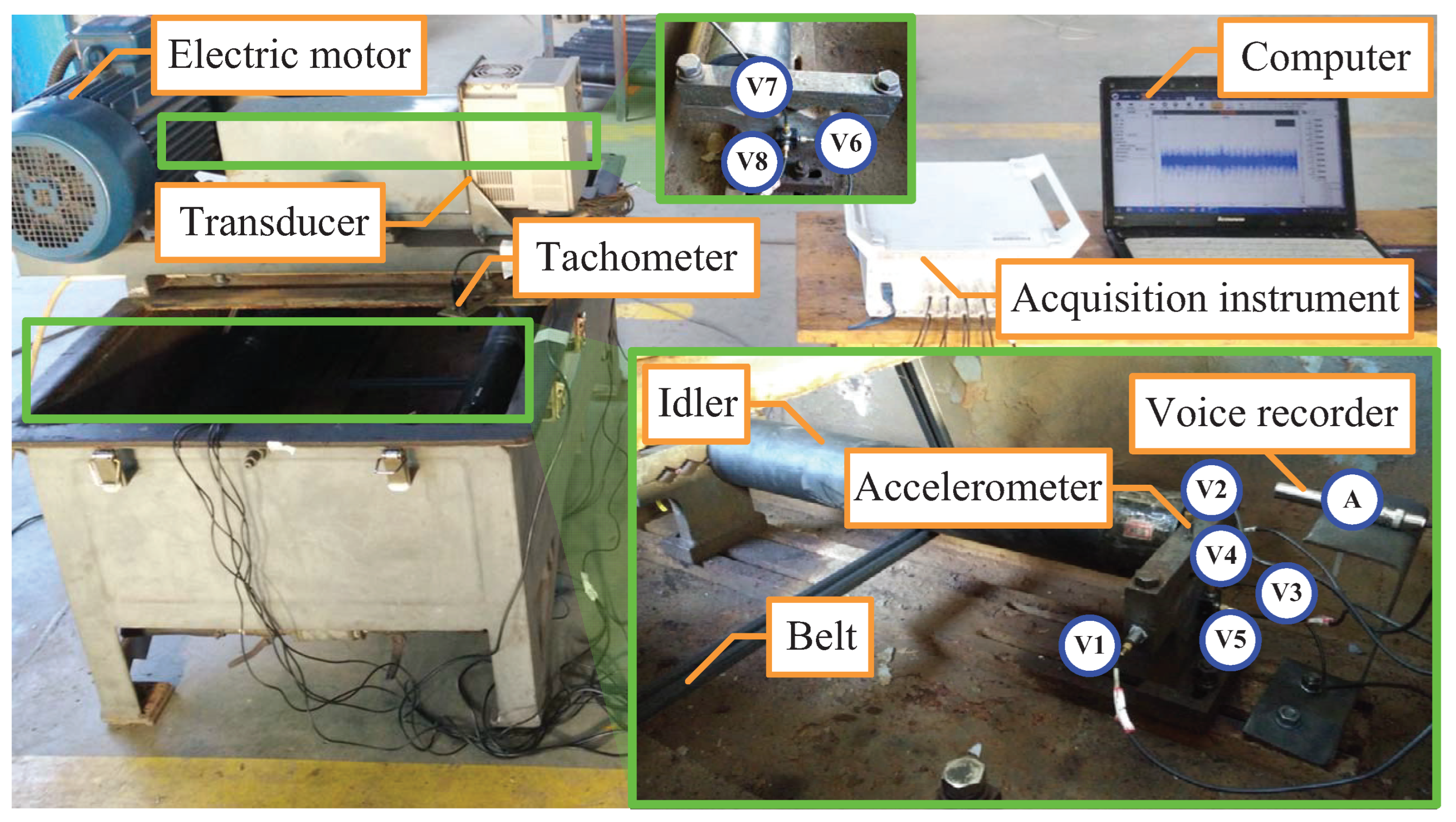
4.1. Experimental Setup and Dataset Preparation

In this section, the experiments were implemented on a fault-simulation testbed of the belt conveyor idler [3]. The testbed shown in Figure 2 mainly consisted of an electric motor for driving, a transducer, a belt, an idler, a tachometer, eight accelerometers, a voice recorder, an acquisition instrument, and a computer. The driving motor was controlled by a transducer with a fixed load and synchronized with a belt, and the idler was driven through the intermediate belt. The defective bearing located in the bearing housing in the idler was further away from the motor, and the other bearing without defects was closer to the motor. Since it was not possible to directly measure the displacement on the bearings, accelerometers were mounted on the bearing housing. In order to acquire the bearing multi-view dataset, a voice recorder was placed around the bearing housing. Finally, the bearing multi-view dataset of the belt conveyor idler, including the raw vibration and acoustic signals, were used to diagnose faults.

In order to develop the proposed fault diagnosis method, inner-race faults (IF), outer-race faults (OF), and ball faults (BF) were manufactured with the help of electrostatic discharge machining. The vibration and acoustic signals were collected simultaneously with a sampling frequency of 20 kHz and 48 kHz, respectively, as illustrated in Figure 2, and each fault type contained four kinds of working conditions, i.e., L0 = 300 rpm, L1 = 600 rpm, L2 = 900 rpm, and L3 = 1080 rpm. In addition, the vibration and acoustic signals of normal bearings (NO) under different working conditions were also considered. The type of bearing utilized was 6204, and its main parameters are displayed in

Table 1. Main parameters of the 6204 ball bearing.

Type	Inner Race	Outer Race	Number	Bearing	Balls
	Diameter (mm)	Diameter (mm)	of Balls	Width (mm)	Diameter (mm)
6204	20	47	8	14	7.9

.

In this experiment, the vibration signals collected by the accelerometer constitute the vibration signal views and the acoustic signals collected by the voice recorder constituted the acoustic signal view. There were eight vibration signal views named V1 to V8 and an acoustic signal view named A. Furthermore, the vibration and acoustic signals were sampled from four kinds of working conditions including L0, L1, L2, and L3, and the vibration signal views under certain working conditions and acoustic signal view under certain working conditions constituted the bearing multi-view dataset of the belt conveyor idler; then, the multi-view datasets including 36 views were constructed in this work. Each sample from each view contained 2049 data points generated by implementing FFT. There were four kinds of health conditions for each view, and each bearing health condition contained 200 samples, that is, each view was composed of 800 samples. In our work, we fixed $\gamma =1$, and the KNN classifier with K was set to 5. In the selection of the parameters of DAML, an empirical search of the parameter space was applied to find the optimal parameter settings. Finally, $k=0.19$ for the feature extraction and fault diagnosis. According to [40], the optimal dimensionality of a feature space is $c-1$ for c class problems. In addition, it is believed that the accuracy of statistical pattern classifiers increases as the number of features increases [42]. Taken together, the dimensionality of the feature space was set to $c=4$.

To demonstrate the effectiveness of DAML, the methods of a-f were compared simultaneously. The scenario settings of all experiments were trained by the labeled samples randomly collected from a multi-view dataset to classify the remaining unlabeled test samples in this multi-view dataset. Three levels that proportion $p_r$ of random selection were considered in each multi-view fault diagnosis test. In all, 384 multi-view fault diagnosis tests were carried out under different sample size conditions, and the details of the experimental scenario are described in

Table 2. Description of the experimental setup.

Vibration Signal	Acoustic Signal	Working	Health	Random Selections
View	View	Conditions	Conditions	${\mathit{p}}_{\mathit{r}}$ (%)
V1	A	L0, L1	NO, IF	10, 30, 70
		L2, L3	OF, BF
V2	A	L0, L1	NO, IF	10, 30, 70
		L2, L3	OF, BF
V3	A	L0, L1	NO, IF	10, 30, 70
		L2, L3	OF, BF
V4	A	L0, L1	NO, IF	10, 30, 70
		L2, L3	OF, BF
V5	A	L0, L1	NO, IF	10, 30, 70
		L2, L3	OF, BF
V6	A	L0, L1	NO, IF	10, 30, 70
		L2, L3	OF, BF
V7	A	L0, L1	NO, IF	10, 30, 70
		L2, L3	OF, BF
V8	A	L0, L1	NO, IF	10, 30, 70
		L2, L3	OF, BF

.

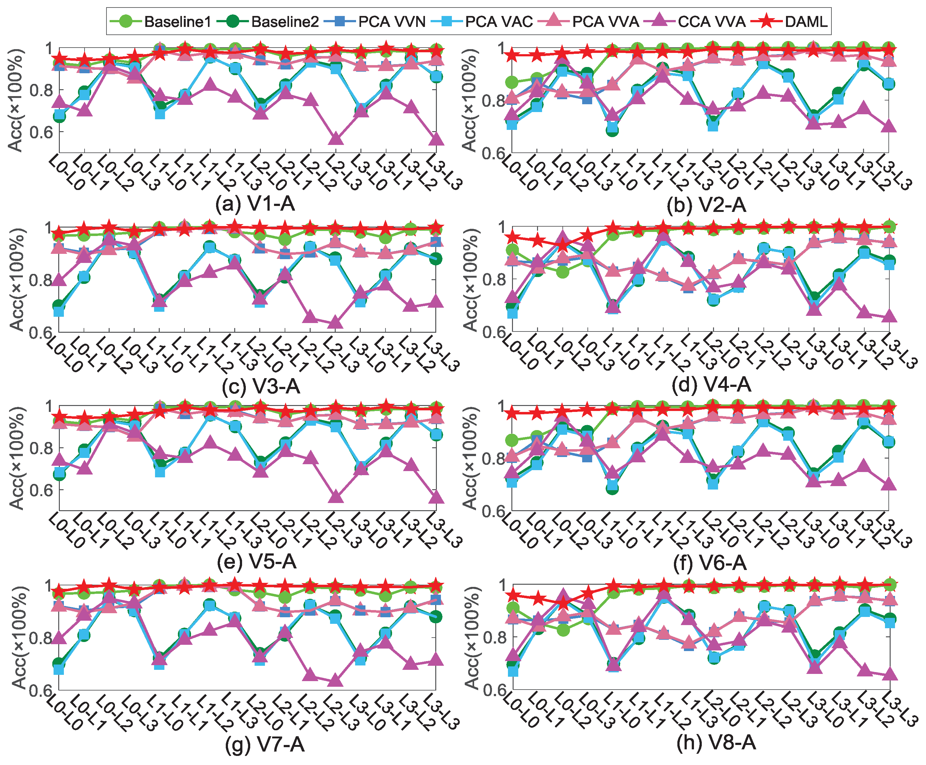
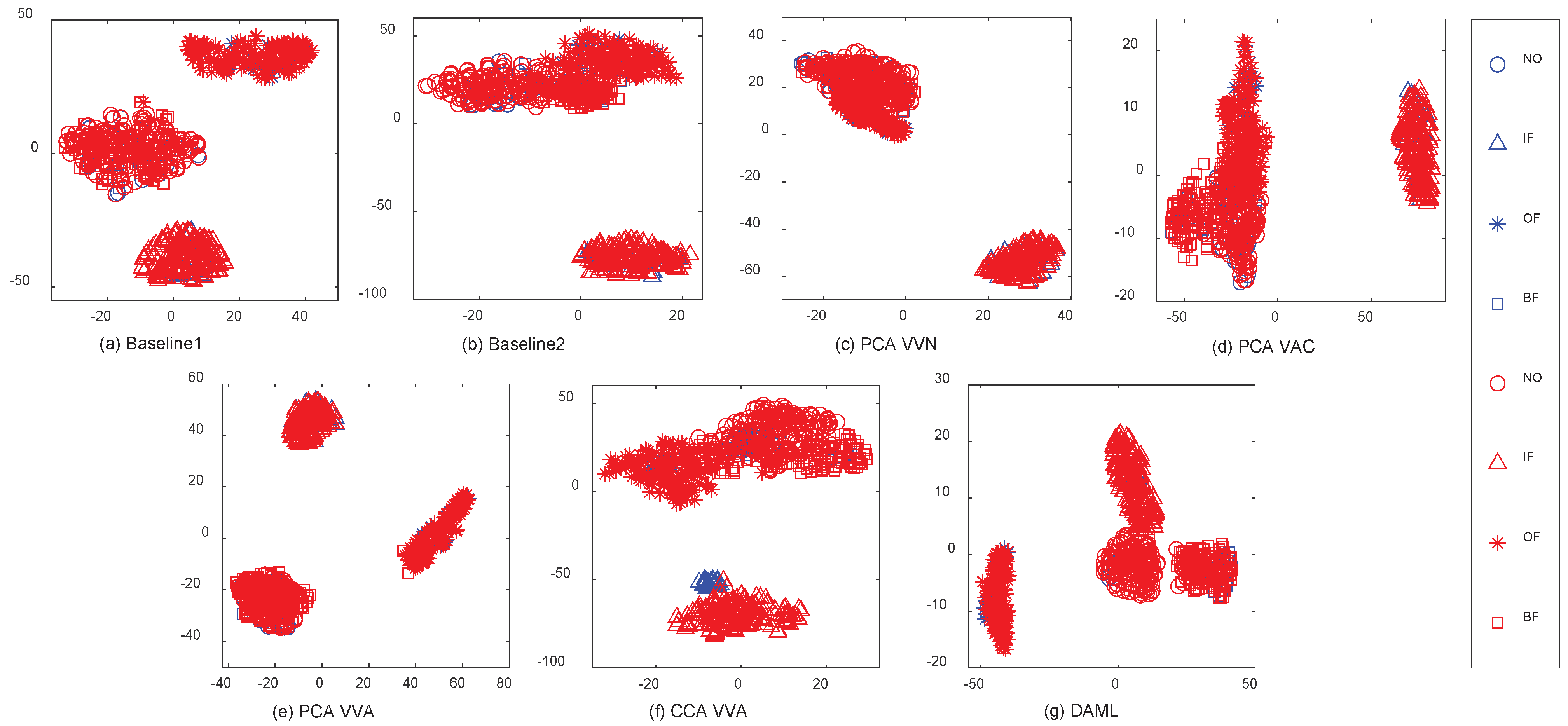
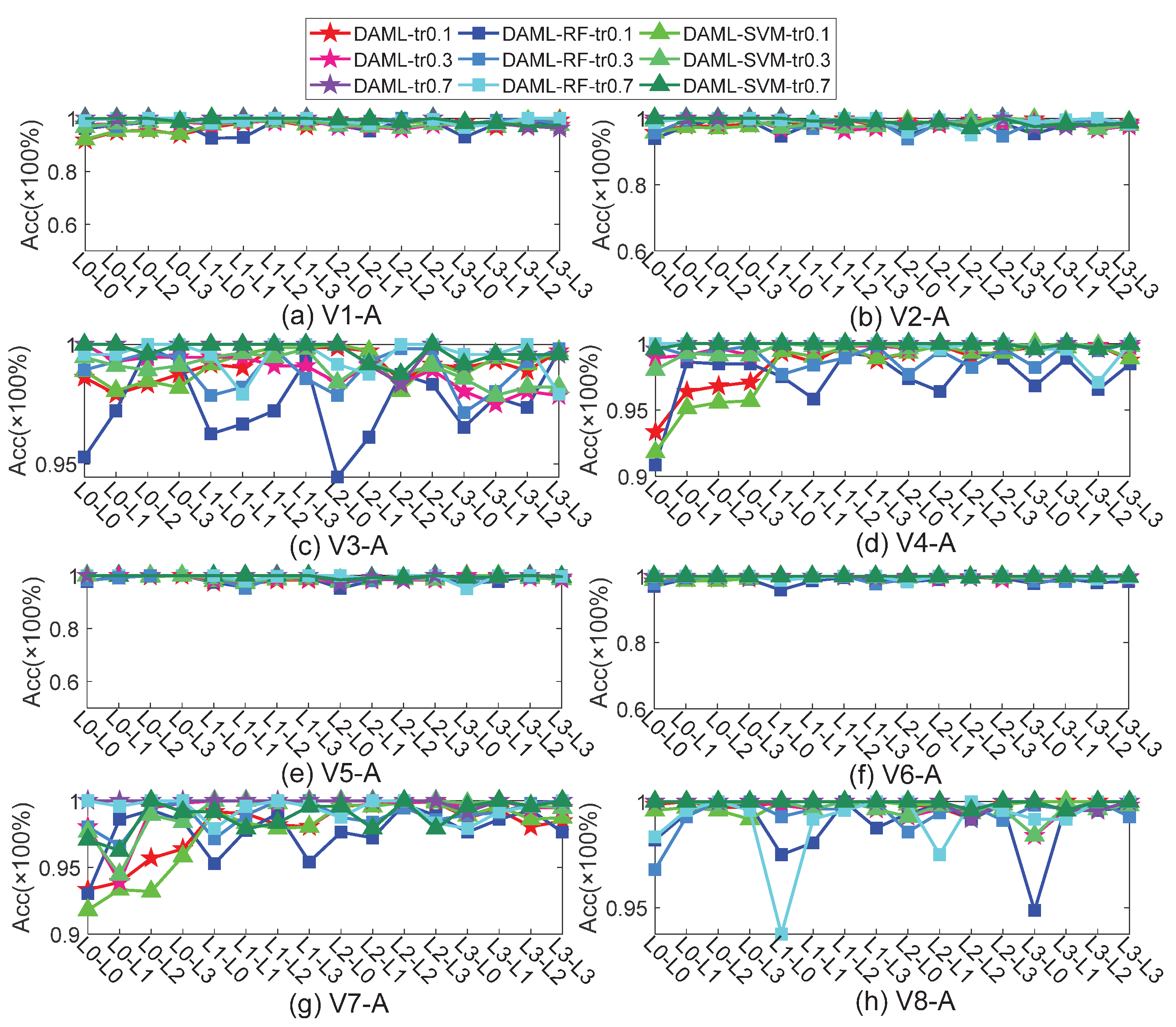
4.2. Diagnosis Results of the Proposed Method

The diagnostic results under the different sample size conditions are shown in Figure 3, Figure 4 and Figure 5. Each figure is composed of eight subfigures involving various combinations from different views. In each figure, the left side of the “-” symbol represents the view from the vibration signals, and the right side represents the view from the acoustic signals. In each subfigure, the left side of the “-” symbol represents the dataset from the vibration signals under certain working conditions, and the right side represents the dataset from the acoustic signals under the other working conditions. Specifically, a multi-view fault diagnosis test L0-L0 was taken as an example in Figure 3a; the vibration signals from L0 and acoustic signals from L0 were randomly selected according to the preset proportions for building a multi-view dataset and training diagnosis model, and the rest were used for the fault classification. Detection precision, including the average classification accuracy and the stability of detection involving the variances in the classification accuracies, are described in Figure 6 and Figure 7, respectively.

From the results of the multi-view fault diagnosis tests shown in Figure 3, Figure 4 and Figure 5, it is clear that fault diagnosis accuracy increased with the increase in the sample size for the mentioned methods, and this trend is more pronounced in Figure 6. To be specific, Baseline 1 was better than Baseline 2 and this phenomenon was reasonable because the acoustic signal was more likely to be contaminated than the vibration signal. For Baseline1, the results generated by the combination of the different views had certain differences, particularly under small sample size conditions. For example, the diagnostic results from (b), (d), (f), and (h) are obviously different to those from (a), (c), (e), and (g) in Figure 3, and performance of Baseline 1 only reached about 80% in “L0-L2” in Figure 3d,h. As far as Baseline 2 is concerned, no matter the conditions, there were large fluctuations in terms of the diagnostic results. PCA VVN was superior to PCA VAC and this was the same with Baselines 1 and 2. Though dimensionality reduction by PCA can preserve the intrinsic information of bearings, the fault feature is always submerged and distorted by relatively strong background noise. In this experiment, Baseline 1 was better than PCA VVN and Baseline 2 was slightly better than PCA VAC. In multi-view diagnostic technology applications, CCA VVA had obvious fluctuations and its stability in detection was the worst. PCA VVA had obvious advantages over CCA VVA, especially when the sample size was large, as shown in Figure 4 and Figure 5. Although PCA VVA was also superior to Baseline 2, PCA VVN, and PCA VAC overall, which can be seen in Figure 6, and its stabilities of detection also had certain advantages, which can be seen in Figure 7, PCA VVA had no advantage over Baseline 1.

To our surprise, DAML clearly outperformed the others. In Figure 4 and Figure 5, it can be seen that the diagnostic accuracies of DAML exceeded 97% in the different multi-view tests, and the vast majority of performances were almost 100% or even achieved 100%. Under the conditions of a 30% training sample size and a 70% training sample size, the average accuracies of DAML reached 99.12% and 99.58%, respectively, which can be seen in Figure 6. As far as the stabilities of detection are concerned, the fluctuations in DAML were only 0.9942 and 0.7064, respectively, which are shown in Figure 7. It is worth noting that DAML could always accurately detect faults no matter what kinds of multi-views were under the condition of a 10% training sample size. More specifically, the average accuracy of DAML under the above conditions was up to 98.77% and the corresponding fluctuation was just 1.3986.

4.3. Discussion

The key to effective fault diagnosis is the construction of view-invariant and category discriminative features from different views. In order to illustrate the superiority of DAML and explain why DAML works, we followed the t-SNE technique [43] to visualize the high-dimensional features of the aforementioned methods in our experiment in a two-dimensional map. For all of the aforementioned cases, a multi-view test “L0-L3”, as seen in Figure 3b, was used as an example in Figure 8 for our discussion and the feature properties from the different views were analyzed under a small sample condition. From the data in Figure 8, it can be seen that there were feature pattern confusions of various degrees when the features were extracted from a single view. Although PCA VVA and CCA VVA extracted features from different views, the above problem was not solved. Theoretically, by benefiting from jointly seeking the most relevant relationships and optimal discriminant features with minimum redundancy in a common subspace, DAML is view-invariant and category discriminative. From the results in Figure 8, it is observable that the multi-view features of DAML were strong clustering and of sufficiently good discrimination.

To further demonstrate the superiority of the view-invariant and category discriminative features extracted from the vibration and acoustic signals, two other classification methods, including random forest and support vector machine, were added for contrast. For illustration, we used the multi-view fault diagnosis tests with different training sample sizes as examples, as seen in Figure 9 and Figure 10, for the discussion.

In Figure 9, the symbols “tr0.1”, “tr0.3”, and “tr0.7” represent the 10% training sample size, 30% training sample size, and 70% training sample size, respectively. DAML-RF and DAML-SVM mean that the extracted features based on DAML were classified with random forest and support vector machine, respectively. From Figure 9, it is clear that DAML, DAML-RF, and DAML-SVM all achieved higher competitive performances than the above-mentioned compared methods. It is worth mentioning here that the extracted features using DAML, DAML-RF, and DAML-SVM were still diagnosed accurately even under the condition of a 10% training sample size. In Figure 10, although it can be seen that there were slight differences in the diagnostic performances, DAML, DAML-RF, and DAML-SVM all showed obvious superiority. It was remarkable that unlike deep learning-based methods that depend on lots of training samples and are time-consuming, the proposed method automatically diagnosed faults accurately based on view-invariant and category discriminative features via max-relevance and min-redundancy, even under the condition of a small training sample size. These results verify that DAML is a promising approach to improving the performance of bearing fault diagnosis.

5. Conclusions

In this paper, discriminant analysis using multi-view learning for bearing fault diagnosis has been proposed. Multi-view feature representation, including view-invariant and category discriminative information, was constructed by jointly seeking the most relevant relationships and optimal discriminant features with minimum redundancy in a common subspace, and the features extracted from a small amount of training samples were successfully used for diagnosis. The proposed method provides a novel perspective for solving the performance degradation problem of a fault classification caused by a single view. Different multi-view fault diagnosis tests demonstrated the effectiveness and feasibility of the proposed method.

Future research will include extending the proposed method to data fusion from more views involving motor currents, torques, and strain gauges. In addition, bearing or gear compound fault diagnoses based on multi-view learning will also be further studied.

References

1. Yi, W.; Guanghua, X.; Ailing, L.; Lin, L.; Kuosheng, J. An online tacholess order tracking technique based on generalized demodulation for rolling bearing fault detection. J. Sound Vib. 2016, 367, 233–249. [Google Scholar]
2. Wang, L.; Wood, R.J.K.; Harvey, T.J.; Morris, S.; Powrie, H.E.G.; Care, I. Wear performance of oil lubricated silicon nitride sliding against various bearing steels. Wear 2003, 255, 657–668. [Google Scholar] [CrossRef]
3. Tong, Z.; Li, W.; Zhang, B.; Jiang, F.; Zhou, G. Bearing Fault Diagnosis Under Variable Working Conditions Based on Domain Adaptation Using Feature Transfer Learning. IEEE Access 2018, 6, 76187–76197. [Google Scholar] [CrossRef]
4. Jiao, J.; Zhao, M.; Lin, J. Unsupervised Adversarial Adaptation Network for Intelligent Fault Diagnosis. IEEE Trans. Ind. Electron. 2020, 67, 9904–9913. [Google Scholar] [CrossRef]
5. Liu, X.; Azzam, B.; Harzendorf, F.; Kolb, J.; Schelenz, R.; Hameyer, K.; Jacobs, G. Early stage white etching crack identification using artificial neural networks. Forsch. Im Ingenieurwesen 2021, 85, 153–163. [Google Scholar] [CrossRef]
6. Zhang, H.; He, Q. Tacholess bearing fault detection based on adaptive impulse extraction in the time domain under fluctuant speed. Meas. Sci. Technol. 2021, 31, 074004. [Google Scholar] [CrossRef]
7. He, Q.; Ding, X. Sparse representation based on local time–frequency template matching for bearing transient fault feature extraction. J. Sound Vib. 2016, 370, 424–443. [Google Scholar] [CrossRef]
8. Chen, L.; Zhenya, W.; Bo, Z. Intelligent fault diagnosis of rolling bearing using hierarchical convolutional network based health state classification. Adv. Eng. Inform. 2017, 32, 139–151. [Google Scholar]
9. Sun, R.B.; Yang, Z.B.; Zhai, Z.; Chen, X.F. Sparse representation based on parametric impulsive dictionary design for bearing fault diagnosis. Mech. Syst. Signal Process. 2019, 122, 737–753. [Google Scholar] [CrossRef]
10. Jardine, A.K.; Lin, D.; Banjevic, D. A review on machinery diagnostics and prognostics implementing condition-based maintenance. Mech. Syst. Signal Process. 2006, 20, 1483–1510. [Google Scholar] [CrossRef]
11. Tian, J.; Morillo, C.; Azarian, M.; Pecht, M. Motor Bearing Fault Detection Using Spectral Kurtosis-Based Feature Extraction Coupled with K-Nearest Neighbor Distance Analysis. IEEE Trans. Ind. Electron. 2016, 63, 1793–1803. [Google Scholar] [CrossRef]
12. Gao, S.; Xu, L.; Zhang, Y.; Pei, Z. Rolling bearing fault diagnosis based on intelligent optimized self-adaptive deep belief network. Meas. Sci. Technol. 2020, 31, 055009. [Google Scholar] [CrossRef]
13. Xu, X.; Lei, Y.; Li, Z. An Incorrect Data Detection Method for Big Data Cleaning of Machinery Condition Monitoring. IEEE Trans. Ind. Electron. 2020, 67, 2326–2336. [Google Scholar] [CrossRef]
14. Samanta, B.; Nataraj, C. Use of particle swarm optimization for machinery fault detection. Eng. Appl. Artif. Intell. 2009, 22, 308–316. [Google Scholar] [CrossRef]
15. Li, Y.; Xu, M.; Wei, Y.; Huang, W. A new rolling bearing fault diagnosis method based on multiscale permutation entropy and improved support vector machine based binary tree. Measurement 2016, 77, 80–94. [Google Scholar] [CrossRef]
16. Chen, R.; Tang, L.; Hu, X.; Wu, H. Fault Diagnosis Method of Low-Speed Rolling Bearing Based on Acoustic Emission Signal and Subspace Embedded Feature Distribution Alignment. IEEE Trans. Ind. Inform. 2021, 17, 5402–5410. [Google Scholar] [CrossRef]
17. Yao, J.; Liu, C.; Song, K.; Feng, C.; Jiang, D. Fault diagnosis of planetary gearbox based on acoustic signals. Appl. Acoust. 2021, 181, 108151. [Google Scholar] [CrossRef]
18. Al-Ghamd, A.M.; Mba, D. A comparative experimental study on the use of acoustic emission and vibration analysis for bearing defect identification and estimation of defect size. Expert Syst. Appl. 2006, 20, 1537–1571. [Google Scholar] [CrossRef] [Green Version]
19. Tandon, N.; Yadava, G.S.; Ramakrishna, A.K. A comparison of some condition monitoring techniques for the detection of defect in induction motor ball bearings. Mech. Syst. Signal Process. 2007, 21, 244–256. [Google Scholar] [CrossRef]
20. Eftekharnejad, B.; Carrasco, M.; Charnley, B.; Mba, D. The application of spectral kurtosis on Acoustic Emission and vibrations from a defective bearing. Mech. Syst. Signal Process. 2011, 25, 266–284. [Google Scholar] [CrossRef] [Green Version]
21. Dingcheng, Z.; Edward, S.; Mani, E.; Clive, R.; Dejie, Y. Intelligent acoustic-based fault diagnosis of roller bearings using a deep graph convolutional network. Measurement 2020, 156, 107585. [Google Scholar]
22. Fei, C.W.; Choy, Y.S.; Bai, G.C.; Tang, W.Z. Multi-feature entropy distance approach with vibration and acoustic emission signals for process feature recognition of rolling element bearing faults. Struct. Health Monit. 2017, 17, 156–168. [Google Scholar] [CrossRef]
23. Peng, B.; Bi, Y.; Xue, B.; Zhang, M.; Wan, S. Multi-View Feature Construction Using Genetic Programming for Rolling Bearing Fault Diagnosis [Application Notes]. IEEE Comput. Intell. Mag. 2021, 16, 79–94. [Google Scholar] [CrossRef]
24. Madhusudana, C.K.; Kumar, H.; Narendranath, S. Fault Diagnosis of Face Milling Tool using Decision Tree and Sound Signal. Mater. Today Proc. 2018, 5, 12035–12044. [Google Scholar] [CrossRef]
25. Shi, H.; Li, Y.; Bai, X.; Zhang, K.; Sun, X. A two-stage sound-vibration signal fusion method for weak fault detection in rolling bearing systems. Mech. Syst. Signal Process. 2022, 172, 109012. [Google Scholar] [CrossRef]
26. Mohanty, S.; Gupta, K.K.; Raju, K.S. Hurst based vibro-acoustic feature extraction of bearing using EMD and VMD. Measurement 2018, 117, 200–220. [Google Scholar] [CrossRef]
27. Iqbal, M.; Madan, A.K. CNC Machine-Bearing Fault Detection Based on Convolutional Neural Network Using Vibration and Acoustic Signal. J. Vib. Eng. Technol. 2022, 10, 1613–1621. [Google Scholar] [CrossRef]
28. Wang, X.; Mao, D.; Li, X. Bearing fault diagnosis based on vibro-acoustic data fusion and 1D-CNN network. Measurement 2021, 173, 108518. [Google Scholar] [CrossRef]
29. Li, C.; Sanchez, R.V.; Zurita, G.; Cerrada, M.; Cabrera, D.; Vásquez, R.E. Gearbox fault diagnosis based on deep random forest fusion of acoustic and vibratory signals. Mech. Syst. Signal Process. 2016, 76–77, 283–293. [Google Scholar] [CrossRef]
30. Yan, X.; Hu, S.; Mao, Y.; Ye, Y.; Yu, H. Deep multi-view learning methods: A review. Neurocomputing 2021, 448, 106–129. [Google Scholar] [CrossRef]
31. Zhao, J.; Xie, X.; Xu, X.; Sun, S. Multi-view learning overview: Recent progress and new challenges. Inf. Fusion 2017, 38, 43–54. [Google Scholar] [CrossRef]
32. Ding, Z.; Shao, M.; Fu, Y. Robust Multi-view Representation: A Unified Perspective from Multi-view Learning to Domain Adaption. In Proceedings of the Twenty-Seventh International Joint Conference on Artificial Intelligence, IJCAI-18, Stockholm, Sweden, 13–19 July 2018; pp. 5434–5440. [Google Scholar]
33. Kan, M.; Shan, S.; Zhang, H.; Lao, S.; Chen, X. Multi-View Discriminant Analysis. IEEE Trans. Pattern Anal. Mach. Intell. 2016, 38, 188–194. [Google Scholar] [CrossRef]
34. Yang, M.; Deng, C.; Nie, F. Adaptive-weighting discriminative regression for multi-view classification. Pattern Recognit. 2019, 88, 236–245. [Google Scholar] [CrossRef]
35. Zhang, C.; Cui, Y.; Han, Z.; Zhou, J.T.; Fu, H.; Hu, Q. Deep Partial Multi-View Learning. IEEE Trans. Pattern Anal. Mach. Intell. 2022, 44, 2402–2415. [Google Scholar] [CrossRef]
36. Wang, Q.; Ding, Z.; Tao, Z.; Gao, Q.; Fu, Y. Generative Partial Multi-View Clustering With Adaptive Fusion and Cycle Consistency. IEEE Trans. Image Process. 2021, 30, 1771–1783. [Google Scholar] [CrossRef]
37. Hardoon, D.R.; Szedmak, S.; Shawe-Taylor, J. Canonical Correlation Analysis: An Overview with Application to Learning Methods. Neural Comput. 2004, 16, 2639–2664. [Google Scholar] [CrossRef] [Green Version]
38. Sun, S.; Xie, X.; Yang, M. Multiview Uncorrelated Discriminant Analysis. IEEE Trans. Cybern. 2016, 46, 3272–3284. [Google Scholar] [CrossRef]
39. Jin, X.; Zhao, M.; Chow, T.W.; Pecht, M. Motor Bearing Fault Diagnosis Using Trace Ratio Linear Discriminant Analysis. IEEE Trans. Ind. Electron. 2014, 61, 2441–2451. [Google Scholar] [CrossRef]
40. Jin, Z.; Yang, J.Y.; Hu, Z.S.; Lou, Z. Face recognition based on the uncorrelated discriminant transformation. Pattern Recognit. 2001, 34, 1405–1416. [Google Scholar] [CrossRef]
41. Sun, Q.; Zeng, S.; Liu, Y.; Heng, P.; Xia, D. A new method of feature fusion and its application in image recognition. Pattern Recognit. 2005, 38, 2437–2448. [Google Scholar] [CrossRef]
42. Hughes, G. On the mean accuracy of statistical pattern recognizers. IEEE Trans. Inf. Theory 1968, 14, 55–63. [Google Scholar] [CrossRef]
43. van der Maaten, L.; Hinton, G. Visualizing Data using t-SNE. J. Mach. Learn. Res. 2017, 9, 2579–2605. [Google Scholar]
Figure 1. The framework of the proposed DAML method.
Mathematics 10 03889 g001
Figure 2. Bearing test platform of the belt conveyor idler.
Mathematics 10 03889 g002
Figure 3. Diagnostic results under the condition of a 10% training sample size, (a) V1-A, (b) V2-A, (c) V3-A, (d) V4-A, (e) V5-A, (f) V6-A, (g) V7-A and (h) V8-A.
Mathematics 10 03889 g003
Figure 4. Diagnostic results under the condition of a 30% training sample size, (a) V1-A, (b) V2-A, (c) V3-A, (d) V4-A, (e) V5-A, (f) V6-A, (g) V7-A and (h) V8-A.
Mathematics 10 03889 g004
Figure 5. Diagnostic results under the condition of a 70% training sample size, (a) V1-A, (b) V2-A, (c) V3-A, (d) V4-A, (e) V5-A, (f) V6-A, (g) V7-A and (h) V8-A.
Mathematics 10 03889 g005
Figure 6. Average classification accuracies under different training sample size conditions.
Mathematics 10 03889 g006
Figure 7. Stabilities of detection under different training sample size conditions.
Mathematics 10 03889 g007
Figure 8. Feature visualization via t−SNE [43] of a multi-view fault diagnosis task, (a) Baseline 1, (b) Baseline 2, (c) PCA VVN, (d) PCA VAC, (e) PCA VVA, (f) CCA VVA and (g) DAML.
Mathematics 10 03889 g008
Figure 9. Diagnosis results of DAML with different classification methods, (a) V1-A, (b) V2-A, (c) V3-A, (d) V4-A, (e) V5-A, (f) V6-A, (g) V7-A and (h) V8-A.
Mathematics 10 03889 g009
Figure 10. (a) Average classification accuracies of DAML with different classification methods; (b) Stabilities of DAML with different classification methods.
Mathematics 10 03889 g010