1. Introduction
Algorithm Trading emerged in the FX spot market in the early-2000s and the Bank of International Settlement (2020) estimated that algorithmic trading transactions account for approximately 20% (USD 400 billion) of daily spot FX volume. Much effort has been invested into improving the algorithm by using Artificial Intelligence in recent years. Therefore, the rising interest in algorithmic trading, machine learning, and reinforcement learning necessitate the need for new meaning input features because the inputs to the models across these studies are too similar [
1].
One of the major meaningful input features could be Support Resistance (SR) Levels. SR is being taught as one of the must-know tools in Technical Analysis. As of the time of writing, SR is taught in every of Amazon’s top sellers’ materials related to Technical Analysis [
2,
3,
4,
5,
6,
7,
8,
9] and is widely used by practitioners. However, there is no formal quantitative definition of SR being established [
10].
According to Osler (2000), there are several common facets in viewing SR levels based on a variety of information such as visual assessments of price movements, numerical rules, order flow, and market psychology [
11]. In other words, SR appeals to many technical analysts. As a result, a popular belief is the power of agreement. The power of agreement suggests that the strength of an SR level is dependent on how many analysts agree to it. However, contrary to the power of agreement, Osler (2000) found that the strength of an SR level is independent of the number of agreed analysts [
11]. This finding motivated this study to explore and engineer new systematic methods to automatically identify meaningful SR levels. More studies are adopting increasingly advanced model architectures and techniques, but the input across these studies is very similar [
1]. The input features commonly used are OHLC prices, volume, and technical indicators. Therefore, the purpose of engineering a systematic and automatic method to identify meaningful SR levels is to leverage the increasing interests and rapid advancement of Artificial Intelligence technology by making SR input features accessible to existing and future intelligent algorithm trading research efforts.
In short, this study aims to improve model predictive performance by introducing new input features that can better explain price movements. These new input features are the SR features engineered from a novel deterministic approach. The objective of this study has 3-fold. Firstly, this study proposes a novel methodology for deterministic SR-level identification. Secondly, this study proposes a methodology to engineer SR features from the identified SR levels to improve price movement prediction measured by execution precision (Equation (7)), f1-score, and profitability. Finally, this study aims to provide empirical evidence of the incremental improvements contributed by the SR input features.
2. Literature Review
Past studies used a combination of neural networks and technical analysis to predict asset price movements [
12,
13]. The rapid adoption of neural networks may be attributed to their non-linearity and non-reliance on prior knowledge about the functional form as it does not require assumptions about data distribution [
14]. According to a survey conducted by Ozbayoglu, Gudelek, and Sezer (2020), past studies mainly use asset prices, technical indicators, and volume as input features to the model [
1]. Although more recent studies started adopting more advanced techniques such as reinforcement learning, the input features across these studies are very similar.
Support Resistance Levels are commonly taught in financial trading books Analysis [
2,
3,
4,
5,
6,
7,
8,
9] and are widely applied by practitioners [
10,
11,
15,
16]. However, SR in particular is an uncommon topic in scientific studies. This may be because the identification of SR varies across analysts as SR identification relies heavily on personal perception and visualization [
17].
Although very limited past studies explicitly define SR as an input to a model, several recent studies have attempted to allow the model to indirectly extract some form of SR information without explicitly defining SR as an input feature via time-series to image conversion techniques [
18,
19]. This technique may be inspired by simulating a human analyst’s visual assessment of price patterns and mainly uses Convolution Neural Network (CNN) as the main model. Sezer and Ozbayoglu (2017) constructed an image representation of a time series by converting 15 technical indicators derived from stock prices with 15 days lag times series into a 15 × 15 matrix [
20]. The matrix is then fed into a 3-class classification convolution neural network that outputs a score on whether the model should ‘Buy’, ‘Sell’, or ‘Hold’ the underlying asset. Hatami (2018) also uses similar classification convolution neural networks but converts a time series into a matrix via a technique known as Recurrence Plots [
19].
Past studies that use time-series to image conversion techniques suggested hidden price patterns may have contributed positively to performance [
18,
19], the degree of contribution of price pattern features towards model performance cannot be assessed since price patterns are not explicitly defined and no direct comparison is conducted between 2 identical models with and without the SR input features, respectively. To carry out this comparison, methods used to explicitly identify and engineer SR features should be explored.
2.1. Methods Used for Support Resistance Identification
During the early days of FX algorithmic trading, Osler (2000) proposed a mechanical method to identify SR levels [
11]. She referred to the SR levels identified by her method as artificial SR. The artificial SR is defined as follows:
where
t = time;
I = ith SR level;
ati and bti = random variables drawn from uniform distribution (0, 1);
range = max gap during the month;
gap = max(open–low, high–open) for a given day.
Osler (2000) studied the relationship between SR levels published by various major FX trading firms, artificial SR, and price behavior [
11]. She also observed several metrics derived from SR and price, such as the average distance between price and SR levels, the average gap between current spot rates and outermost Support and Resistance Levels, and the number of agreed levels (where agreed levels are defined as SR levels that is published by more than 1 firm).
Osler (2000) provided statistical evidence that SR levels have predictive power over intraday price movements [
11]. More interestingly, the author also found that agreed levels are not stronger than SR published by a single firm, implying “there’s no power in agreement”. Since the author’s findings suggested there’s no power in agreement, new methods to identify a meaningful SR should be explored.
Another approach to identifying SR is an intelligent method such as Evolutionary optimization algorithms [
15,
16]. The evolutionary optimization algorithm is a subset of Artificial Intelligence and Soft Computing. Evolutionary optimization algorithms are commonly used for optimizing parameters and are also being adopted to optimize parameters for Technical Indicators [
21,
22], asset allocation strategies [
23], and algorithmic trading parameters [
20,
24].
Some findings suggest that evolutionary optimization algorithms may be effective in determining optimal parameters for Technical Indicators [
21,
22], but the findings related to using evolutionary optimization algorithmic to identify SR levels were not appealing [
15,
16].
Besides that, Mayo (2013) suggested that the SR levels detected by Differential Evolution Algorithm only performed better than randomly selected SR levels in liquid markets based on price penetration probability [
15]. Yıldırım, Uçar, and Özbayoğlu (2019) used the SR levels identities by evolutionary optimization algorithm as buying and selling signals on 5 Exchange-Traded Funds (ETF) [
16]. They found that this strategy does not outperform the buy-hold strategy on 4 out of 5 ETFs. However, this only suggests that the strategy contributed no improvement, but no conclusion can be drawn whether SR contribute to any incremental improvement in performance.
2.2. Summary of Past Studies Related to Support Resistance Identification
Firstly, past studies examined the performance of trading strategies derived from the identified SR based on various methods such as mechanical methods [
11] or soft computing methods [
15,
16], but not the direct incremental contribution of SR by comparing the performance of 2 identical intelligent models with and without the SR input features, respectively.
Secondly, the 2 drawbacks of the current methods discussed are as follows:
The stochastic nature of evolutionary optimization algorithms yields indeterministic output each time the algorithm is trained, even if the hyperparameters are kept constant [
25]. This may yield inconsistent evaluation and also inconsistent results during comparison. On the other hand, mechanical methods yield deterministic results as the output. The stability of the mechanical method is more suitable for comparison and evaluation purposes.
Osler’s (2000) artificial SR is an early day example of mechanically identifying SR levels [
11]. However, SR is often determined by connecting highs and lows to form horizontal lines or zones Analysis [
2,
3,
4,
5,
6,
7,
8,
9], a feature not defined and captured by Osler’s (2000) mechanical method.
Therefore, the purpose of this study is to propose a novel mechanical method to overcome to two drawbacks stated above and examine the incremental contribution of SR (Psychological Price Levels) input by directly comparing two identical intelligent models with and without the SR Input Features, respectively.
3. Methodology
3.1. Novel Mechanical Method for Identifying Support Resistance
This study proposes a novel SR identification approach that align with the “power of agreement” [
1]. The “power of agreement” suggests that SR levels that receives more public attention outperform arbitrary or privately identified SR levels.
The novelty of our approach is that the SR levels identified are derived from a highly accessible technical indicator (ZigZag). As a result, the identified SR levels are highly visual, reproducible, deterministic, and receive a high degree of attention from other traders and technical analysts. Our unique methodology further processes the identified SR levels into meaningful input features (distance between current price and the 2 next closest SR level). The distance between the 2 closest SR level represents the amount of room available for an asset price (exchange rates) to move in one direction before risking bouncing off into the opposite direction that would otherwise hit the take profit or stop loss price.
Finally, unlike past studies, intelligent methods are used to extract the relationship between price movements and the identified SR levels. In other words, intelligent model such as neural networks to learn the association between the SR levels and price movements. This approach has advantage over past studies in the aspect of application. The proposed approach involves end-to-end learning where the model learns relevant information from the identified SR levels to automatically make better trade decisions. Whereas past studies attempt to better apply the identified SR levels through experimenting with different rule-based algorithm [
11,
15,
16].
The novel mechanical method proposed in this study identifies SR levels based on connecting swing highs and lows. Therefore, swing high and swing low endpoints are first identified. This study proposes a Swing High Swing Low Detection Algorithm (SHSLDA) inspired by the Zig Zag Indicator where the swing highs and swing low endpoints are mechanically identified via a function of Depth, Deviation, and Backstep.
A candidate SR is identified when a connection is established between 2 endpoints or between an existing candidate or validated SR and an endpoint. A connection is established when the price distance between 2 endpoints or the existing candidate or validated SR is less than a threshold known as span. Whenever a connection is established, the resulting SR level is the average price of all connected endpoints. In addition, the number of connected endpoints and the time distance since the latest endpoint associated with the candidate or effective SR are tracked.
A candidate’s SR is considered validated if 2 of the following conditions are met:
Number of connected endpoints must be more than an arbitrary number (default = 2);
The time distance (number of candles/periods) from the latest connection established cannot exceed an arbitrary number of periods (default = 100).
3.2. Novel Feature Engineering on Support Resistance
Only validated SR levels are considered in the modeling process. Two validated SR (SR) levels are determined at every observation, 1 support level, and 1 resistance level. For a long (buy) position, the support level is the nearest SR below the entry price whereas the resistance level is the nearest SR above the entry price. For a short (sell) position, the support level is the nearest SR above the entry price whereas the resistance level is the nearest SR below the entry price.
Then, the distance between the support level and the entry price level and the distance between the resistance level and the entry price level is computed. The raw validated SR price levels are not used as input features. Instead, the input features are engineered to be the distances between the entry prices price and the raw validated SR price levels.
Since resistance can reverse price movements [
11,
15,
16], this engineered input feature can provide the model with relevant information to determine whether the price can move ahead to hit the take-profit price level or reverse within a specified time window when there’s a resistance level(s) ahead. Similarly, this engineered input feature can also provide the model with relevant information to determine whether the price will move ahead to hit the stop loss price level or reverse within a specified time window when there’s support level(s) ahead.
The maximum distance is set to be the distance between the take profit (TP) price and the entry price (EN) or the distance between the stop loss (SL) price and the entry price (EN) to avoid infinity numerical error. If there is no validated support or resistance price level, the distance between the entry price and the take profit price or stop loss price is used.
3.3. Other Input Features
Four of the most traded currency pairs in 2020 according to Statista are included in this study. The 4 currency pairs are EURUSD, USDJPY, GBPUSD, and AUDUSD. Hourly Open-High-Low-Close (OHLC) price data are retrieved from the Dukascopy historical data feed for the period from 22 August 2017 to 28 January 2021. The data is split into a training set and a test set. A total of 80% of the data are allocated to the training set which is used to train the model. The remaining 20% of the data are allocated to the test set which is used for evaluating the out-sample performance of the model. The data are chronologically ordered from oldest to most recent, hence the training set contains older data and the test set contains more recent data.
Three price action features and seven technical indicator features are derived from the retrieved hourly OHLC price data to compliment the SR input feature. The price action variables and their respective computation methods are shown in
Table 1 whereas the technical indicators included are shown in
Table 2.
The Day of Week, Parabolic SAR Signal, and the EMA Crossover Signal variables are categorical variables. Day of Week is a 7-class categorical variable where each value corresponds to a day of the week. Parabolic SAR signal is a 2-class categorical variable. Parabolic SAR Signal = 0 when SAR is lower than Close, whereas Parabolic SAR Signal = 0 when SAR is higher than Close.
EMA Crossover Signals are generated when 2 EMA crossover each other. Each crossover will be assigned a categorical value. The EMA Crossover Signal variable has an arbitrary number of classes depending on how many EMAs are used. The EMA Cross Signals are also direction-specific. In this study, the EMA Crossover Signal is computed based on 3 exponential moving averages (EMAs), which are 9-day EMA, 13-Day EMA, and 21-Day EMA. Since 3 EMAs are used, the EMA Crossover Signal has 12 classes.
Therefore, 13 input variables including 2 SR levels are used as inputs to the model. The lag length of the features used in this study is 64 h which approximates 2.5 days. The lag length used equals the look-ahead window used in generating the ground truth.
3.4. Generating Ground Truth
Take profit (TP) and stop loss (SL) are often used to exit a trade. When TP and SL are used, the trade will have 4 possible outcomes as shown below:
Price hits the SL, and the trade is exited at a loss.
Price hits the TP, and the trade is exited at a profit.
Price did not hit either TP or SL, but the trade is at an unrealized loss.
Price did not hit either TP or SL, but the trade is at an unrealized profit.
Therefore, a 4-class classification model is used to predict the outcome of a trade. The ground truths classes are defined with the following convention:
Ground truth class = 0 if Price exceeds the stop loss price within the look-ahead prediction window.
Ground truth class = 1 if Price exceeds the take profit price within the look-ahead prediction window.
Ground truth class = 2 if the price did not hit either the take profit price or stop loss price but is out-of-the-money.
Ground truth class = 3 if the price did not hit either the take profit price or stop loss price but is In-the-money.
The limitation of this method is the frequency of the data. Since the data collected are on an hourly timeframe, there are instances when the low is lower than the stop loss price and the high is higher than the take profit price simultaneously. This study employs a conservative measure to consider these instances as a loss (class 0) rather than a profit (class 1).
Pip is the basic unit used in measurement changes in exchange rates and 1 pip equals 0.0001 unit for non-JPY-related currency pairs whereas 1 pip equals to 0.01 for JPY-related currency pairs. The TP pips and SL pips used in this study are 90 and 20, respectively. This provides the model with a reward-risk ratio of 4.5. The TP pips and SL pips are used to compute the TP price and SL price for each trade.
3.5. Look Ahead Window
A pre-determined look-ahead window is used to identify the lifespan of a trade. The look-ahead window can prevent a trade from going on indefinitely and provide a well-defined time scope for the prediction. This allows the model to learn a meaningful relationship between the input features and the trade’s outcome. If the look-ahead window is too large, all trades will eventually exit by SL or TP but the outcome cannot be meaningfully mapped to the input features. If the look-ahead window is too small, too many trades will not hit the TP or SL and no meaningful relationship between input features and the trade outcome can be extracted.
The look-ahead window does not have to be arbitrary. The look-ahead window can be a function of timeframe, the volatility of the currency pairs, and the distance of the take-profit price and stop-loss price from the entry price. The look-ahead window can also be based on personal investing preferences such as day trading, scalping, or swing trading. In this case, the timeframe, the volatility of the currency pairs, and the TP pips and SL pips must accommodate the look-ahead window.
This study uses 64 h look-ahead window to approximate 2.5 days or half a week to reflect the authors’ preference for a trade’s life span, hence the TP and SL pips of 90 pips and 25 pips are used, respectively, to accommodate the look-ahead window. These parameters are adopted from previous similar studies [
13] and were further modified to ensure sufficient distance (pips) are provided to between entry price and stop loss price to avoid excessive premature stop out while ensuring that majority of the ground truths are distribution among class-0 and class-1 outcome.
3.6. Normalization
High-frequency exchange rate time series at hourly timeframe is known to be noisy [
26]. It means that the exchange rate’s day-to-day variations are often unpredictable due to sources of demand and supply being too broad. Therefore, the numeric features included in this study are first smoothed by normalizing them into midpoints of bins.
Table 3 illustrates the smoothing convention.
The smoothed numeric features are further normalized by lag-wise MinMag Normalization. MinMag Normalization is a variation of MinMax Normalization without the denominator factor. Hence, the original magnitude of change is retained while mitigating autocorrelation.
The volatility of exchange rate time series is known to be time-dependent [
27]. MinMag Normalization may be better than using MinMax normalization due to time-dependent volatility in time series data such as exchange rate where 20% change during 1 period is not the same as 20% change during another period. Hence, MinMax normalization may mislead the model during training. Moreover, MinMag Normalization also retains the original shape of the visual representation of the time series. This could help the model during training.
MinMag Normalization is defined as below:
Assuming 2-dimensional features with dimension = (lag, features) where lag = features = 3, an example of the resulting normalized features is as below:
3.7. Test Model
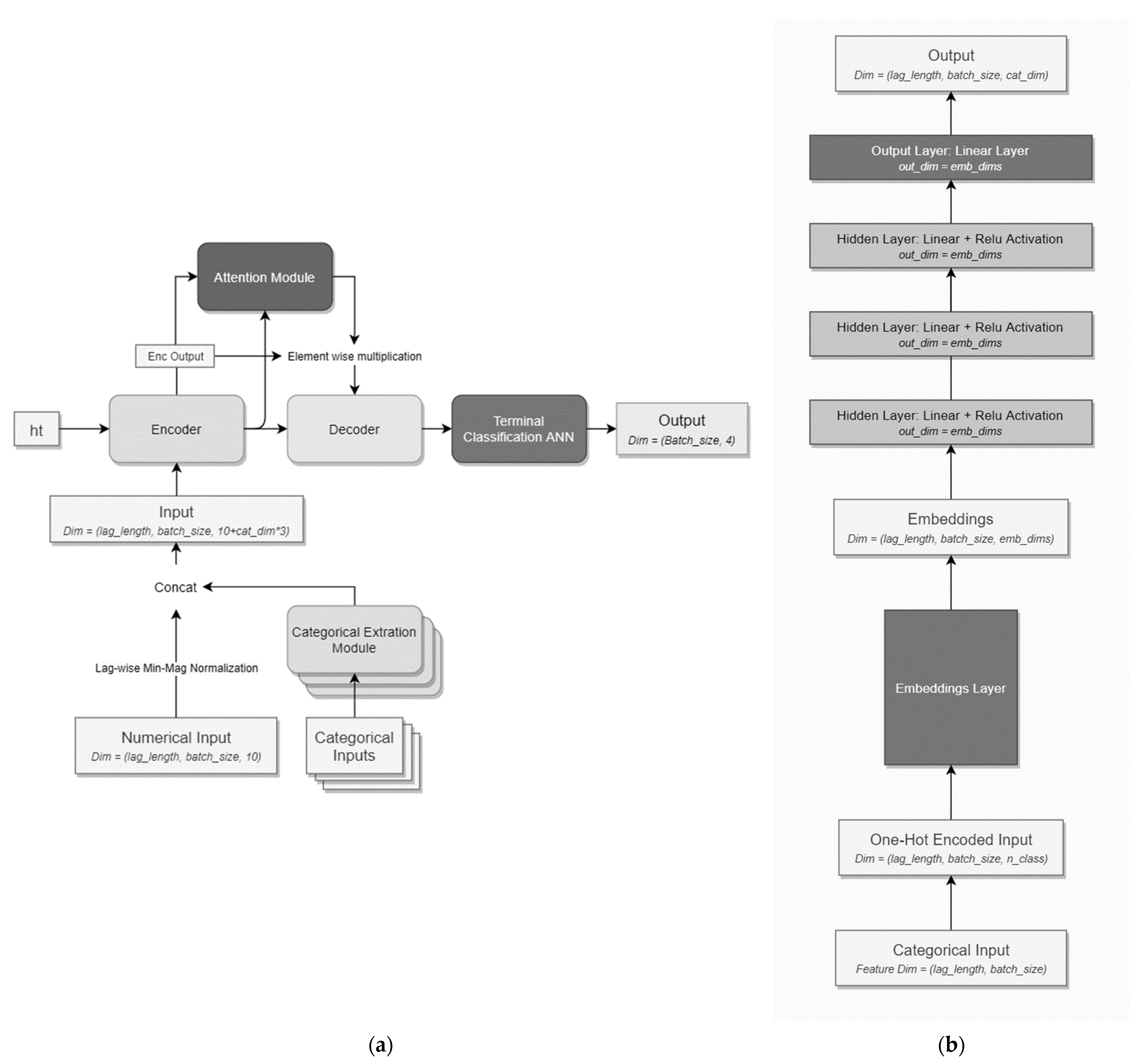
The model’s framework is shown below in
Figure 1a. The model framework consists of 5 modules including the Categorical Feature Extraction Modules (CFEM), the attention module, the Encoder, the Decoder, and a 1-layer terminal classification artificial neural network.
CFEM is composed of an embedding layer, 3 hidden layers, and an output layer with specifications shown in
Figure 1b. The Categorical Feature Extraction Modules are unique for each categorical variable. Since there are 3 categorical variables used in this study, there are 3 CFEMs. The main purpose of the CFEM is to represent a category better via
embdims real numbers instead of a dummy variable or a one-hot encoded variable where
embdims is a positive integer. The features output from the CFEM is then concatenated with the numerical features to form the model input.
The Encoder and Decoder are GRU recurrent neural networks with 5 layers and a hidden size of 3 times the input size. The attention module is a 2-layer artificial neural network with a hidden size equal to the input size. Kaiming normal Initialization [
28] is used to initialize the weights of the 5 modules.
The Focal Loss Function is used to mitigate overfitting [
29]. The Focal Loss Function is a modification to the cross entropy loss function by adding a modulating factor (1 − p
t)
γ where p
t is the classification probability output and γ ≥ 0. Focal Loss reduces the loss contributed by samples that are closer to the ground truth, hence the model is forced to optimize by reducing the loss of the unfitted samples. The Focal Loss Function is defined as below:
Other relevant specifications used are the Adam Optimizer [
30] and Early Stopping. These parameters are adopted from previous similar studies [
13] and were further modified to accommodate categorical variables and embeddings layer which are not present in the previous studies.
3.8. Evaluation Methodology: Class-1 Precision as the Primary Performance Metric
Accuracy is a common metric used to measure performance in a classification task. However, class-1 precision is the main and more important performance metric in algorithmic trading tasks because trade is only executed when the model predicted an outcome class of 1, which is the price will hit the TP price level within the look-ahead window. No loss is incurred for forgoing a trade and a loss is only incurred for executing a losing trade. Hence, the precision of Class-1 Prediction is the primary and the more important performance metric, and minimizing false positives should be the priority before maximizing true positives. In addition to Class-1 prediction precision, F1-score is also included as a secondary metric because it represents the general geometric mean between precision and recall for the predictions of all classes. The computations are defined below.
One limitation to class-1 precision is the interpretability caused differing reward-risk (RR) ratio where a higher RR ratio implies the potential loss severity is less but the chances of a loss are higher. This is because the price has to travel less to hit the stop-loss price level than the take-profit price level. In contrast, the higher the RR ratio, the potential profit is higher, but the chances of profitability are less because the price has to travel more to hit the take profit than the stop loss. In short, the higher the RR ratio the lower the precision, and vice versa.
Due to the differences between the potential profit and potential loss severity, precision may not be an accurate measurement of performance. A model trained with a 4.5 RR ratio is expected to have lower precision than a model trained with a 1 RR ratio, but it does not mean that the model trained with a 4.5 RR ratio underperformed the model trained with a 1 RR ratio. For instance, assuming a base price unit such as 20 pips, the model trained with a 4.5 RR ratio that has 35% precision would have an expected profit of 35% × (4.5 price unit) − 65% × (1 price unit) = 2.225 price unit = 44.5 pips per trade. On the other hand, the model trained with a 1 RR ratio and precision of 60% would only have an expected profit of 65% × (1 price unit) − 35% × (1 price unit) = 0.3 price unit = 6 pips per trade.
For this reason, Profitability is also included as a secondary performance metric. The profit of a sample can be computed using the convention below:
If ground truth class = 0, profit = SL pips;
If ground truth class = 1, profit = TP pips;
If ground truth class is 2 or 3, profit = terminal closing price-entry price, where terminal closing price = the closing price at the end of the look-ahead window.
Training and evaluation will be repeated 10 times for each of the 4 currency pairs. In other words, 10 models will be trained for each currency pair using the training set data, and the profitability of each model on the test set data will be recorded to provide reliable distribution of the performances [
16,
31].
The training and evaluation process mentioned above is to be conducted again using the training set and test set without the SR features. Then, the performance distribution between the model trained with the SR features and the model trained without the SR features are analyzed. t-Test will be used to test the following hypothesis:
H0. The performance between the model trained with SR features and the model trained without SR features is not statistically different.
H1. The performance between the model trained with SR features and the model trained without SR features is statistically different.
4. Results
4.1. Distribution of Performance Metrics
This section discusses the results to illustrate the incremental performances of using the SR features proposed. Ten models with the SR features and ten models without the SR features are trained and evaluated for each currency pair to provide sets of 10 classification errors. This provides better distribution of the performances as the resulting neural network is probabilistic due to initialization methods and parameters optimization algorithm.
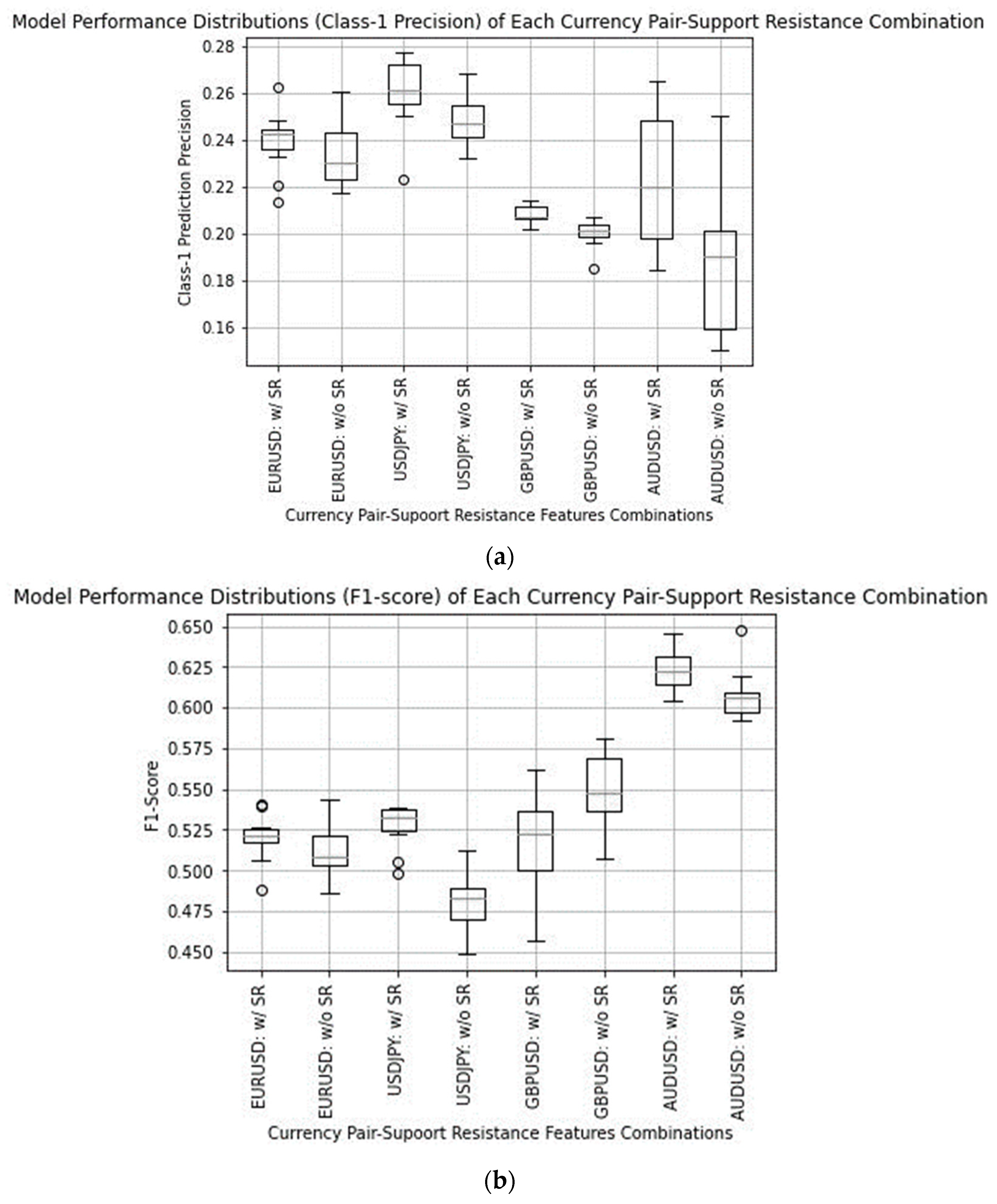
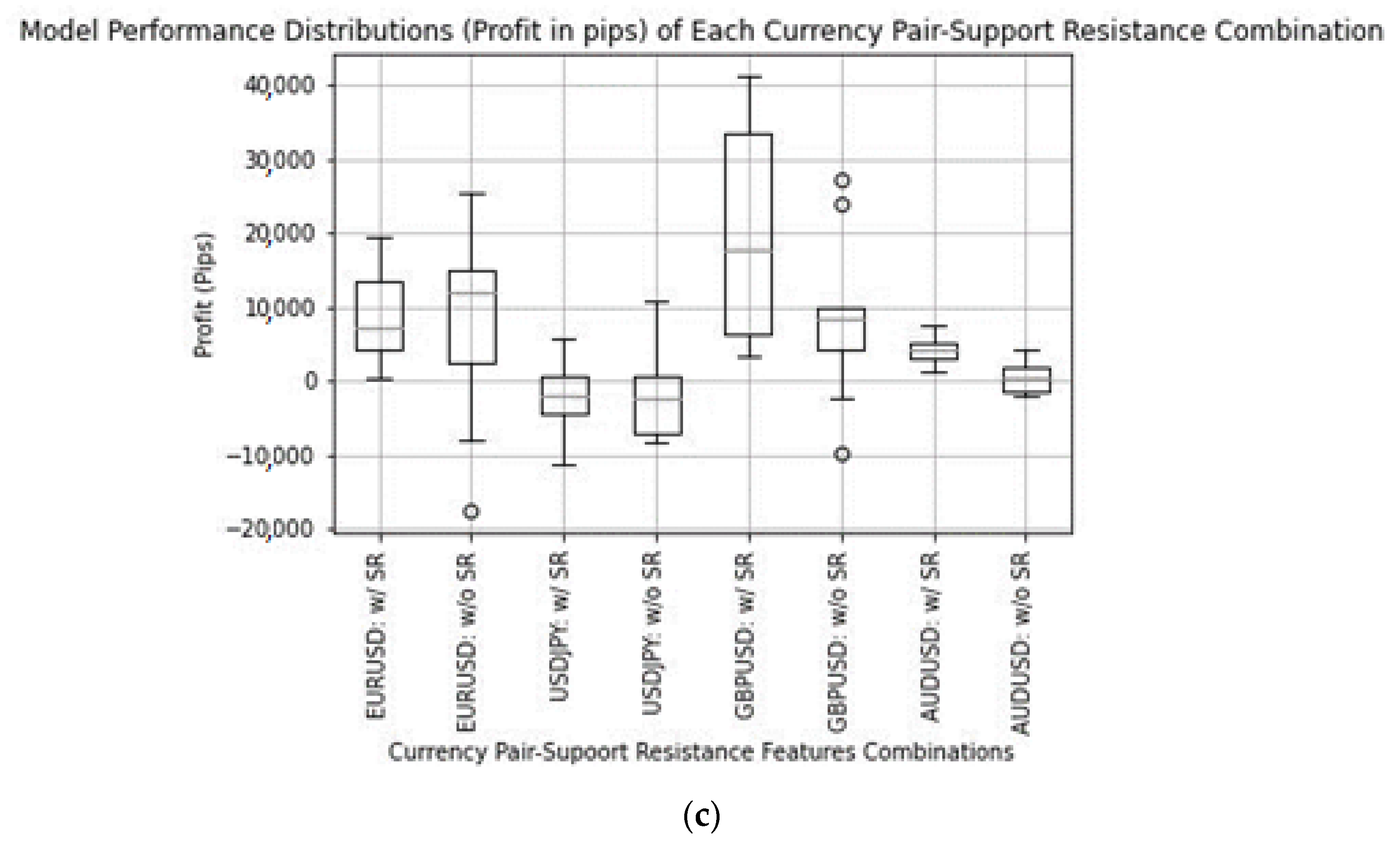
The results of the models are presented in
Figure 2a–c.
Figure 2a represents the performances of the models for each currency with and without the SR based on Precision of Class 1 Predictions.
Figure 2b represents the performances of the models for each currency with and without the SR based on the F1 score.
Figure 2c represents the performances of the models for each currency with and without the SR based on profitability.
Results presented in
Figure 2a–c show the respective precision, f1-score, and profitability of the models with and without SR on the four most traded currency pairs. Each combination of currency pair and usage of SR is represented by a box and whisker vertical bar. The box represents the region between the lower and upper quartiles of the distribution of precision. The horizontal line in the box represents the median of the performance distribution.
It is observable that the proposed SR features improve the model performances in terms of the medians and the general distributions of precision, F1-score, and profitability. The models trained with the proposed SR outperform the models trained without the proposed SR features for all four most traded currency pairs based on the primary performance metric (class-1 precision) and at least three out of four based on f1-score and profitability (secondary performance metrics).
Models trained with the proposed SR feature outperform models trained without the proposed SR features across all four currency pairs in terms of Class-1 prediction precision. Apart from GBPUSD, models trained with the proposed SR feature have higher F1 scores than models trained without the proposed SR features. Lastly, models trained with the proposed SR are also more profitable than models trained without the proposed SR for all currency pairs except EURUSD.
This study’s results align with Osler’s (2000) finding although the results were not directly comparable. This is because the metric used to measure the impact of an identified SR level on price movement is different. Osler (2000) measured the impact based on the probability of exchange rates (GBPUSD and USDJPY) bouncing off an identified SR level (bounce rate) while this study measured the impact by examining the incremental improvement in the model prediction precision. Nevertheless, the implications are the same: the identified SR level affects price movements and therefore should be considered when trading.
Although Osler’s (2000) mechanical method does not satisfy the definition of a SR, which involves connecting high and low, the exchange rates (GBPUSD and USDJPY) had a higher probability of bouncing off the identified SR levels than if no SR levels were identified. Similarly, this study found that the models trained with SR levels have better predictive performance based on class-1 precision, f1-score, and profitability.
This is a stark contrast to the performance of SR levels identified by indeterministic intelligent models such as evolutionary algorithms [
15,
16]. Yildirim, Uçar, and Özbayoğlu (2019) examined the impact of the SR levels identified by evolution algorithms through profitability, which is comparable to this study. However, the authors found that trading with the SR levels identified by the evolution algorithms underperformed a simple buy-hold strategy, implying that the SR levels identified are not impactful. On the other hand, all models trained with the SR levels identified by this study’s proposed approach outperform the models trained without.
According to Osler (2000), the outperformance of both Osler’s (2000) and this study’s proposed strategy can be attributed to the “power of agreement” [
11]. Simply put, the more attention an SR level receive, the more impactful it becomes as investors share similar perception. Osler (2000) found that the bounce rate in publicly published SR levels is significantly higher than arbitrary SR levels identified by the author’s simple rule-based algorithms. This aligns with the results of this study. This is because the SR level identified by this study’s proposed deterministic approach is derived from a commonly accessible technical indicator (ZigZag) and might have more shared attention than indeterministic and visually peculiar SR levels identified by evolutionary algorithms [
15,
16].
4.2. Discrepancy between Class-1 Precision, F1-Score and Profitability
There seems to be a slight discrepancy between Class-1 prediction precision and profitability. For instance, the models trained with the proposed SR have higher precision but lower profitability for EURUSD. This discrepancy is caused by the varying degree of profitability and losses for outcome classes. The degrees of profitability in ascending order are Class 0, Class 2, Class 1, and Class 4. In this study, the model will only execute a trade if it predicts an outcome of Class 1 since a prediction of Class 1 outcome denotes a prediction of a profitable trade. No trades are executed for the prediction of outcome Class 0, Class 2, and Class 3. Profitability could be higher for a given Class-1 prediction precision because a trade could still be profitable even if the prediction is wrong where the actual outcome turns out to be Class 3. On the other hand, profitability could be lower for a given Class-1 prediction precision because incorrect predictions could be more concentrated in Class 0. This iterates the significance of evaluating the model’s performance directly by profitability.
By referring to
Figure 3, it is observable that the incorrect prediction of Class 1 of the model trained with the SR features is more heavily concentrated in Class 0 (largest degree of losses) than the model trained without the SR features for the currency pair EURUSD. Therefore, the profitability from higher Class-1 prediction precision is negated by heavier losses from Class 0-concentrated incorrect prediction.
The discrepancy between class-1 precision and f1-score can be observed as a side effect of forgoing subpar trading signals. Since the models in this study will only execute a trade if the models predict a class-1 outcome, the models could deliberately misclassify a class-1 ground truth as other outcome classes to avoid taking the trade. The misclassification of class-1 outcome as other class outcome does not affect class-1 precision (Equation (7)) but will affect the general precision which considers the precision for all outcome classes (Equation (6)). Nevertheless, results showed minimal impact on f1-score and profitability where the models trained with the SR levels identified by the proposed approach outperform on three out of four datasets based on f1-score and profitability.
4.3. Statistical Significance
Figure 1,
Figure 2 and
Figure 3 showed the distribution of performance metrics for models trained with and without the SR features for the four most traded currency pairs and suggests that the model trained with the proposed SR features outperforms the model trained without the SR features. However, this information alone is not sufficient to show that the difference in performance is statistically significant. Therefore, this section shows that the statistical differences between models trained with and without the SR features are significant.
The statistical difference tests between the models trained with and without the SR are conducted via t-test. Firstly, the t-test is conducted at two levels. The t-test is first conducted to test the statistical differences at the currency level, and then it is tested aggregately across the four most traded currency pairs as an aggregated measurement. The t-test is also performed based on the distributions of three performance metrics, Class-1 precision, F1-Score, and profitability.
By referring to the findings in
Table 4,
Table 5 and
Table 6, the performance differences between models trained with and without the SR features are statistically significant except for profitability on the EURUSD dataset. Aside from the profitability on the EURUSD dataset and F1-score on the GBPUSD dataset, there is sufficient evidence to suggest that the SR features engineered by the proposed approach improve price movement predictions.
5. Conclusions
Support and resistance levels are important in financial trading applications and have been shown to impact price movements. Although recent studies are developing and adopting increasingly advanced model architectures and techniques, the models’ input features across these studies are similar. This study aimed to introduce new features to better predict price movements. Past studies showed that public attention helps validate the strength of an SR level and can explain the underperformance of SR levels identified by indeterministic and intelligent methods. This observation was coined as the “power of agreement” [
11].
Therefore, this study proposed a novel SR identification approach inspired by the highly accessible, reproducible, and deterministic Zig Zag Indicator. Subsequently, the identified SR levels are further processed into input features representing distance available before an asset price bounces towards the opposite direction.
Results showed that the models trained with the SR features engineered from the proposed approach outperform their counterparts trained without the SR features on class-1 precision, f1-score, and profitability. Results also showed that the outperformances are statistically significant. Therefore, there is sufficient evidence to suggest that the SR levels identified and the resulting input features engineered by the proposed approach contributed to the incremental improvement in price movement prediction.


