Article

Dwarf Mongoose Optimization Metaheuristics for Autoregressive Exogenous Model Identification

by
Khizer Mehmood
1,
Naveed Ishtiaq Chaudhary
2,*,
Zeshan Aslam Khan
1,
Khalid Mehmood Cheema
3,
Muhammad Asif Zahoor Raja
2,
Ahmad H. Milyani
4 and
Abdullah Ahmed Azhari
5
1
Department of Electrical and Computer Engineering, International Islamic University, Islamabad 44000, Pakistan
2
Future Technology Research Center, National Yunlin University of Science and Technology, 123 University Road, Section 3, Douliou, Yunlin 64002, Taiwan
3
Department of Electronic Engineering, Fatima Jinnah Women University, Rawalpindi 46000, Pakistan
4
Department of Electrical and Computer Engineering, King Abdulaziz University, Jeddah 21589, Saudi Arabia
5
The Applied College, King Abdulaziz University, Jeddah 21589, Saudi Arabia
*
Author to whom correspondence should be addressed.
Mathematics 2022, 10(20), 3821; https://doi.org/10.3390/math10203821
Submission received: 25 September 2022 / Revised: 12 October 2022 / Accepted: 14 October 2022 / Published: 16 October 2022
(This article belongs to the Special Issue Optimisation Algorithms and Their Applications)

Abstract

:
Nature-inspired metaheuristic algorithms have gained great attention over the last decade due to their potential for finding optimal solutions to different optimization problems. In this study, a metaheuristic based on the dwarf mongoose optimization algorithm (DMOA) is presented for the parameter estimation of an autoregressive exogenous (ARX) model. In the DMOA, the set of candidate solutions were stochastically created and improved using only one tuning parameter. The performance of the DMOA for ARX identification was deeply investigated in terms of its convergence speed, estimation accuracy, robustness and reliability. Furthermore, comparative analyses with other recent state-of-the-art metaheuristics based on Aquila Optimizer, the Sine Cosine Algorithm, the Arithmetic Optimization Algorithm and the Reptile Search algorithm—using a nonparametric Kruskal–Wallis test—endorsed the consistent, accurate performance of the proposed metaheuristic for ARX identification.

1. Introduction

Over recent years, metaheuristic techniques have made substantial progress in the solution of different optimization problems arising in the spectrum of engineering applications [1,2,3,4,5,6,7]. One may classify optimization heuristics into four categories: Group one includes methods inspired by human behavior such as balanced teaching–learning-based optimization [8], harmony searches [9] and socio evolution and teaching–learning optimization [10]. Group two includes evolutionary algorithms involving mutation and crossover operations; a few methods in this area include genetic algorithms [11], differential evolution [12], biogeography-based optimizers [13] and bat algorithms [14,15]. Group three includes physics-based techniques involving physical laws for optimization problem solutions; a few techniques in this area are Henry gas solubility optimization [16,17], the big bang–big crunch [18,19] and gravitational search algorithms [20,21]. The final group includes swarm intelligence-based techniques used for optimization solutions; a few methods in this area are particle swarm optimization [22,23], artificial bee colonies [24,25], cuckoo searches [26,27], the marine predators algorithm [28,29] and the slime mold algorithm [30,31]. Recently, the dwarf mongoose optimization algorithm (DMOA) has been proposed, obtaining better results than standard state-of-the-art algorithms [32,33,34]. Its easy structure, with only controlling parameter, and its better performance motivated the authors to exploit these strengths for the parameter estimation of an autoregressive exogenous noise (ARX) model.
The ARX model is widely used to model a number of engineering optimization problems such as electrical/power systems [35], estimating battery charge [36], predicting electrical loads [37] and forecasting gas emissions and water flooding [38,39,40]. The parameter estimation of the ARX model is of paramount significance owing to its ability to model different phenomena. Some of the parameter estimation methods that have been proposed for ARX identification are recursive identification [41], the variational Bayesian approach [42], the sparse estimation idea [43], momentum gradient descent [44], the variable step-size information gradient scheme [45], the two-stage gradient mechanism [46], evolutionary algorithms [47] and Aquila search optimization [48].
Sörensen exposed the metaphor of proposing novel metaheuristics in his great research work [49] and pointed out some actual research directions in metaheuristics that would take this field a step forward rather than backward. However, the current research study extends the application domain of metaheuristics and provides a detailed investigation into solving the parameter estimation problem of the ARX model through the exploitation of the well-established strengths of the DMOA. A detailed performance evaluation of the proposed scheme for ARX identification was conducted for different noise conditions in the ARX structure. The reliability of the proposed approach in comparison with other recently introduced metaheuristics was established through detailed analyses based on multiple independent experiments and statistical tests.
The remainder of the paper can be outlined as follows: Section 2 describes the ARX model structure. Section 3 presents the DMOA methodology, with pseudocode and flow chart descriptions. Section 4 provides the results of detailed simulations by way of graphical and tabular representations. Finally, Section 5 concludes the study by presenting the main findings of the current investigation.

2. Mathematical Model of ARX Systems

The parameter estimation of the ARX model structure presented in Figure 1 is of great interest for the research community because of its ability to model a variety of real-life problems. Saleem et al. used the ARX structure to model real-life induction motor drive [50]; Azarnejad et al. investigated ARX processes to study the dynamics of an actual stock returns system [51]; Hadid et al. explored the practical applications of ARX in disaster management through effective flood forecasting by rainfall-runoff modelling of rivers [40]; Li et al. exploited the ARX model for the modeling of practical industrial processes such as the pH neutralization process, which is normally required in wastewater treatment [52] and many other processes.
The description of the terms in Figure 1 are as follows: ε ( j ) is the input, θ ( j ) is the output, q ( j ) is random noise and H ( z 1 ) and I ( z 1 ) are polynomials with the degrees n h and n i , respectively, as given in (1) and (2):
H ( z 1 ) = 1 + h 1 z 1 + h 2 z 2 + + h n h z n h ,
I ( z 1 ) = i 1 z 1 + i 2 z 2 + + i n i z n i
The output of the ARX model presented in Figure 1 is given in (3):
θ ( j ) = I ( z 1 ) H ( z 1 ) ε ( j ) + 1 H ( z 1 ) q ( j )
Multiplying (3) by H ( z 1 ) on both sides results in the equation given in (4):
H ( z 1 ) θ ( j ) = I ( z 1 ) ε ( j ) + q ( j )
Equation (4) can be rewritten as:
θ ( j ) = [ 1 H ( z 1 ) ] θ ( j ) + I ( z 1 ) ε ( j ) + q ( j )
Defining the information vectors as in (6) and (7) and the parameter vectors, they can be estimated as shown in (8) and (9):
κ h ( j ) = [ θ ( j 1 ) , θ ( j 2 ) , , θ ( j n h ) ] ,
κ i ( j ) = [ ε ( j 1 ) , ε ( j 2 ) , , ε ( j n i ) ] ,
h = [ h 1 , h 1 , , h n h ]
i = [ i 1 , i 2 , , i n i ]
The identification model for the ARX system can be determined using the overall information and parameter vectors given in (10)–(12), respectively:
θ ( j ) = κ T ( j ) γ + q ( j ) ,
κ ( j ) = [ κ h ( j ) κ i ( j ) ] ,
γ = [ h i ]
The objective was to estimate the parameter vector (12) of the ARX model through the optimization strength of the DMOA scheme.

3. Methodology

In this section, a DMOA-based methodology for the parameter estimation of the ARX model is presented.

3.1. Dwarf Mongoose Optimization Algorithm

The DMOA is a swarm intelligence-based method inspired by animal behavior for the finding of solutions to optimum global problems. It replicates dwarf mongoose behavioral responses. The DMOA model, pseudocode and algorithm flow are presented below.

3.1.1. Population Initialization

The DMOA started with the initialization of the population for mongoose candidate solutions (S), as given in (13):
S = [ s 1 , 1 s 1 , Q s N p , 1 s N p , Q ]
N p is the total population size and Q is the number of decision variables or the features of the dwarf mongoose. The number of decision variables Q for the parameter estimation problem of the ARX system represents the parameters of the ARX system provided in the parameter vector γ , as given in (12). The population is generated randomly using (14):
S u , v = unifrnd ( LB , UB , Q )
LB   and   UB are the lower and upper bounds of the problem.

3.1.2. The DMOA Model

The optimization procedure of the DMOA was divided into three groups, which are presented below.

Alpha Group

After the initialization, the population fitness of each solution was calculated using (15). On the basis of fitness, the female alpha was chosen, as presented in (15):
α = fit j j = 1 N p fit j
As the number of mongooses in α is related to the number of babysitters bb and the vocalization of the dominant female ρ , the solution’s updated mechanism was calculated using (16):
S j + 1 =   S j + ρ
is the distributed random number. The sleeping mound was calculated for every repetition using (17):
ε j = fit j + 1   fit j max { | fit j + 1 ,   fit j | }
The average of ε j was calculated using (18):
σ = j = 1 N p ε j N p
The algorithm moved to the next group when the babysitter criteria was met.

Scout Group

During this phase, if the family forages far enough, then a new sleeping mound will be discovered—this was calculated using (19a) and (19b):
if   θ j + 1 >   θ j :   S j + 1 = S j DF rand [ S j V ]
e l s e   :   S j + 1 = S j + DF rand [ S j V ]
Here, the rand value was between [ 0 ,   1 ] . DF was a parameter for controlling the collective volitive movement of the mongoose group and V was the movement vector; they were both calculated using (20) and (21):
DF = ( 1 m max _ G ) ( 2 m max _ G ) ,
V = j = 1 N p S j × ε j S j

The Babysitters

The babysitters are the secondary group that stays with youngsters. To assist the alpha female, babysitters are recycled on a routine basis, while the rest of the squad conducts daily hunting expeditions. The pseudocode of the DMOA is presented in Algorithm 1. The flowchart for the DMOA is shown in Figure 2.
Algorithm 1: Pseudo-code of the DMOA
Initialization:
Initialize   DMOA   parameters :   population   N p   and   number   of   babysitters   bb .
Set N p = N p bb .
Set babysitter exchange parameter K .
for m = 1 : max _ G
Calculate the mongoose fitness.
Set   time   Counter   D .
Calculate α = fit j j = 1 N p fit j
Calculate   candidate   food   position   S j + 1 =   S j + ρ .
Evaluate   new   fitness   of   S j + 1 .
Evaluate   sleeping   mound   ε j = fit j + 1   fit j max { | fit j + 1 ,   fit j | }
Compute   average   of   ε j . σ = j = 1 N p ε j N p .
Compute movement vector V = j = 1 N p S j × ε j S j .
Exchange babysitters if D K and set.
Initialize bb position usng (1) and calculate fitness fit j α .
Simulate next position S j + 1 = { S j DF rand [ S j V ]     if   θ j + 1 > θ j     Exploration S j + DF rand [ S j V ] else     Exploration
Update best solution
end
Return best solution
End

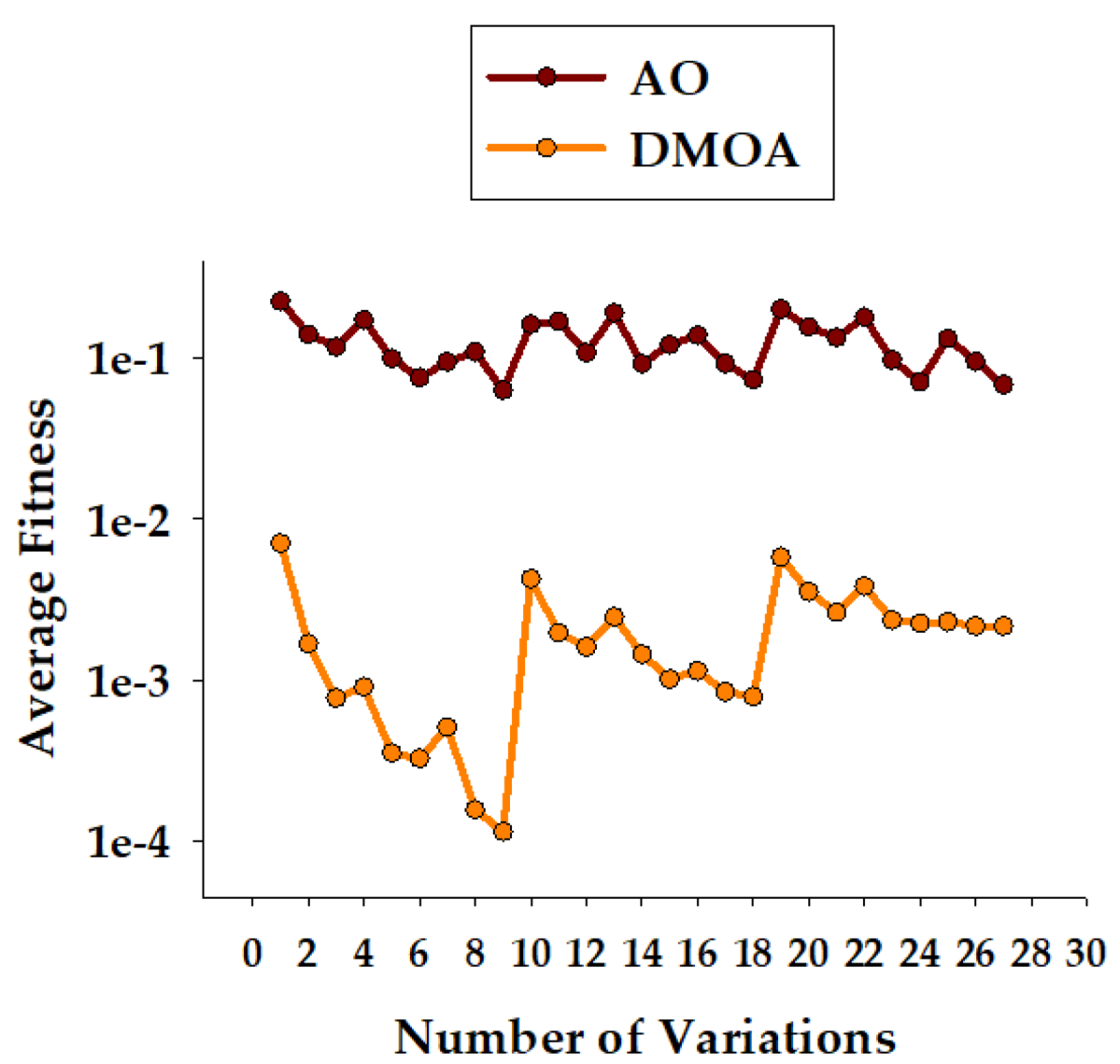
4. Performance Analysis

In this section, the performance analysis of the DMOA for the ARX model is presented. The identification of the ARX model was conducted over several noise levels, generations and population sizes. The algorithm was evaluated in terms of its accuracy, as measured by the fitness function presented in (22):
Fitness   Function = mean ( θ θ ^ ) 2
Here, θ ^ is the estimated response determined by the DMOA and θ is the desired response or actual output of the ARX model as presented in (12). For the simulation study, we considered the second order ARX model presented in (23) and (24). The simulations were conducted in Matlab with the input as a zero mean unit variance signal, and the desired output was obtained using the desired parameters provided in Equations (23) and (24) of the ARX system. Meanwhile, the noise signal was considered to be zero with a normal distribution, having a constant variance.
H ( z 1 ) = 1 1.5 z 1 + 0.7 z 2 ,
I ( z 1 ) = 1.0 z 1 + 0.5 z 2

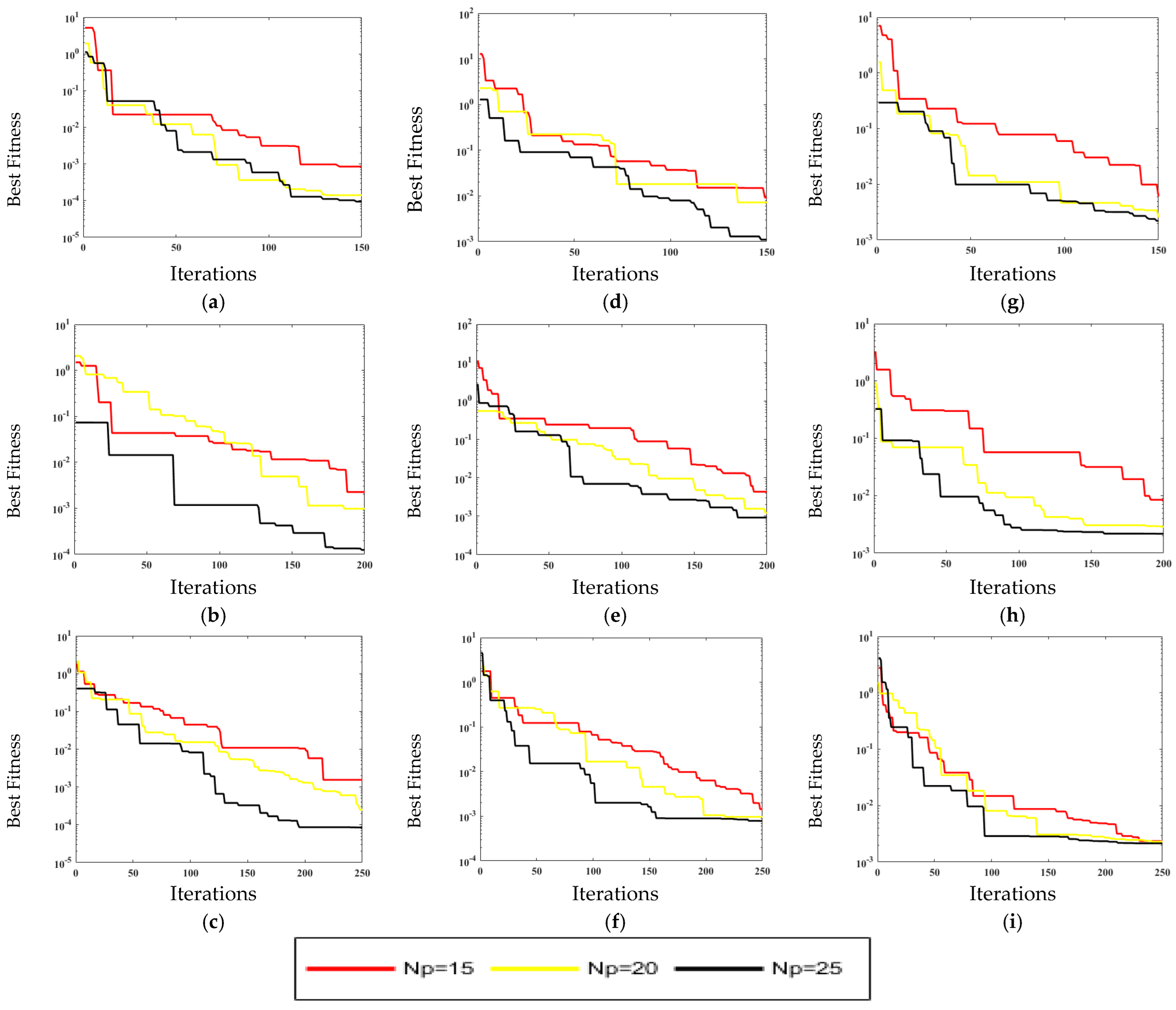
4.1. Statistical Convergence Analysis

In this section, the performance of the DMOA is judged by introducing three noise levels to the ARX model. The simulations were conducted in a MATLAB Windows 10 environment. The parameter settings of the DMOA for the ARX model were: number of babysitters bb = 3, babysitter exchange parameter K = 7 and female vocalization α = 2. Moreover, the fitness of the DMOA was valued through three variations of generation number (150, 200 and 250) and population size (15, 20 and 25). The Average Fitness, Best Fitness, Worst Fitness and standard deviation (STD) were the evaluation metrics used to evaluate the performance of the DMOA for the ARX model.
The performance in terms of the number of babysitters bb is presented in Table 1. It can be seen from the table that by increasing bb , the average fitness increased for all population numbers and generation sizes. The best values achieved for Average Fitness, Best Fitness and Worst Fitness were 1.1 × 10 4 , 8.5 × 10 5   and   2.6 × 10 4 at a population size of 25, a generation size of 250 and bb = 3.
The performance in terms of fitness variations and standard deviations for the three noise levels, i.e., 0.01, 0.03 and 0.05, is demonstrated in Table 2, Table 3 and Table 4, respectively. It can be seen from Table 2, Table 3 and Table 4 that the fitness of the DMOA decreased with increasing population size and number of generations. It is notable in Table 2 that the minimum Average Fitness, Best Fitness and Worst Fitness achieved for the noise level = 0.01 were   1.1 × 10 4 , 8.5 × 10 5 and 2.6 × 10 4 , respectively. Similarly, the three best fitness values for the noise levels 0.03 and 0.05—given in Table 3 and Table 4—were 7.9 × 10 4 , 7.6 × 10 4   and   8.9 × 10 4 and 2.2 × 10 3 , 2.1 × 10 3   and   2.6 × 10 3 , respectively.
The performance of the DMOA method in terms of Best Fitness for the three noise levels, i.e., 0.01, 0.03 and 0.05, was evaluated for three variations in the number of generations (150, 200 and 250) and population size (15, 20 and 25); the fitness plots are shown in Figure 3. The fitness curves in Figure 3a–c represent the Best Fitness of the DMOA algorithm for noise variance = 0.01. In contrast, Figure 3d–f signifies the Best Fitness curves for noise variance = 0.03. Likewise, the Best Fitness plots for noise variance = 0.05 are given in Figure 3g–i. It can be observed from Figure 3a–i that the fitness of the DMOA for the three noise levels, i.e., 0.01, 0.03 and 0.05, was reduced significantly with increases in population size and the number of generations. However, better results with regard to fitness were achieved with lower values of noise, a greater number of generations and larger population sizes.
To confirm the natural behavior of the DMOA for different noise values, the performance of the DMOA was also verified by fixing the population size (15, 20 and 25) and changing the generation size (150, 200 and 250) for three values of noise variance (0.01, 0.03 and 0.05); the fitness-based learning curves are presented in Figure 4. Figure 4a–c represents the Fitness achieved by the DMOA with population size = 15. However, the fitness plots for population size = 20 are given in Figure 4d–f, while Figure 4g–i denotes the fitness plots for population size = 25. It can be seen from the fitness curves given in Figure 4a–i that for a fixed population size and number of generations, the fitness achieved by the DMOA for low levels of noise, i.e., 0.01 and 0.03, was quite low compared to the fitness for a high noise level, i.e., 0.05. Yet, the DMOA achieved the minimum value of fitness for the smallest value of noise, i.e., 0.01, for a fixed population size. Therefore, it is confirmed from the curves in Figure 4 that the performance of the DMOA was lower with higher noise values.

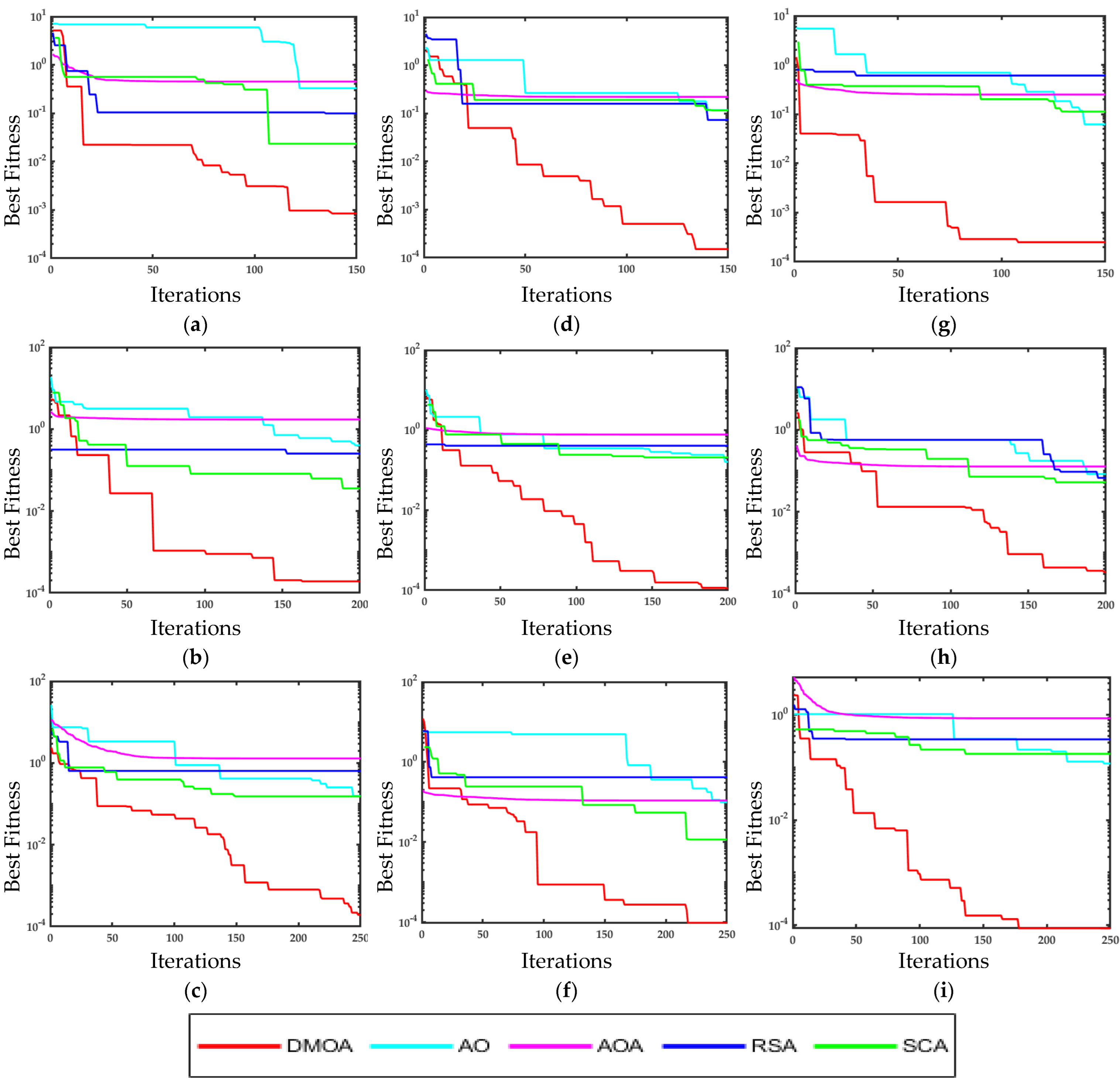
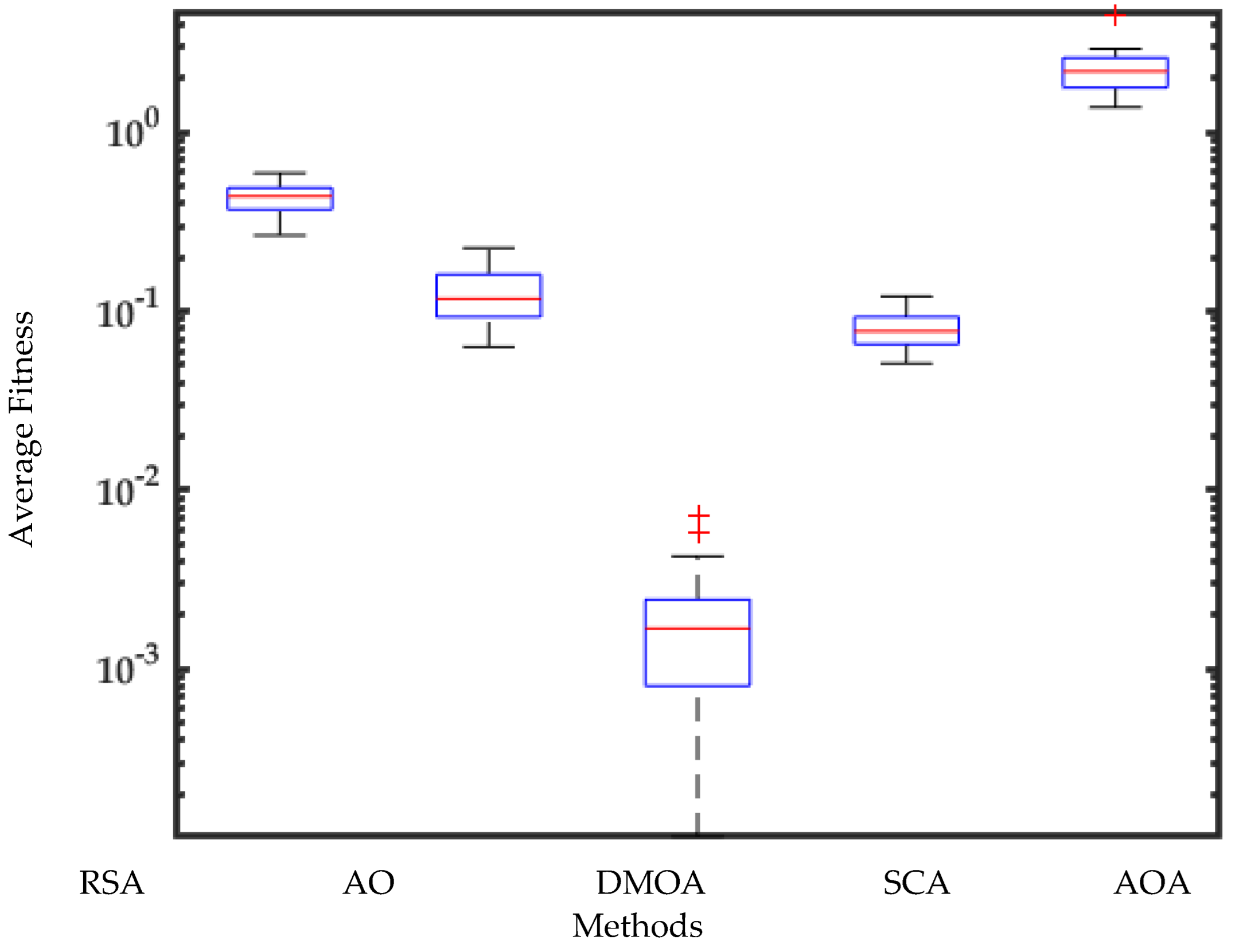
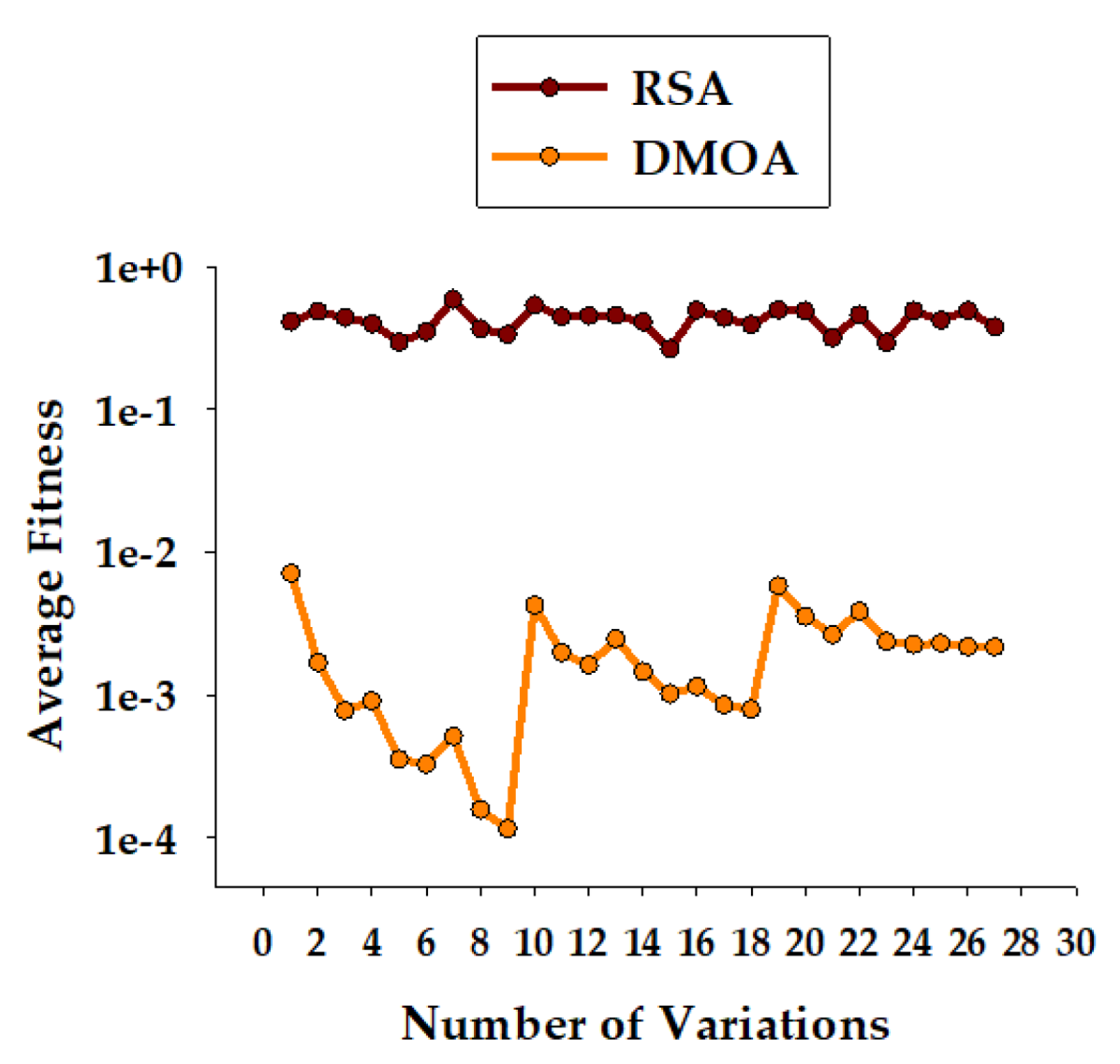
4.2. Results Comparison with Other Heuristics

To further investigate the DMOA, it was compared with other swarm intelligence-based methods including Aquila optimizer (AO) [53], the reptile search algorithm (RSA) [54], the sine cosine algorithm (SCA) [55] and the arithmetic optimization algorithm (AOA) [56] for 30 independent runs, with multiple variations of generation number (150, 200 and 250) and population size (15, 20 and 25) considered. These methods were selected in terms of their performance in solving engineering optimization problems and their source code availability. Brief descriptions and the parameter settings of these methods are summarized in Table 5.
The performance of the DMOA method in terms of Best Fitness was compared with the AO, AOA, RSA and SCA for the three variations in generation number (150, 200 and 250) and population size (15, 20 and 25); the fitness plots are shown in Figure 5. The fitness curves in Figure 5a–c represent the Best Fitness of the DMOA algorithm for Np = 15. In contrast, Figure 5d–f signifies the Best Fitness curves for Np = 20. Likewise, the Best Fitness plots for Np = 25 are given in Figure 5g–i. The noise variance is shown in Figure 5a–I is 0.01. It can be observed from Figure 5a–I that the fitness of the DMOA was lower for all variations compared to other methods. Moreover, the fitness value decreased with increasing population size and numbers of generations.
Table 6, Table 7 and Table 8 show the performance of all the algorithms in terms of their estimated weights and best fitness values for the 0.01, 0.03 and 0.05 noise variances. It can be seen that for lower noise variances, i.e., 0.01, the algorithm gave better results compared to higher noise variances. Moreover, for low noise variances, the estimated weights were closer to true values, with minimum fitness values.
The statistical analysis of the DMOA, AO, AOA, SCA and RSA for multiple runs—with noise variances, population sizes, and constant generation sizes—are shown in Figure 6. It can be seen that for all noise variances, the DMOA achieved lower fitness compared to the AOA, SCA, RSA and AO. It can also be observed that by increasing the noise level, the performance of all the algorithms degraded. However, the DMOA achieved optimal fitness in all scenarios.
Figure 7 shows a comparison of the boxplots for the average fitness values of the DMOA against those of the AO, AOA, RSA and SCA for all variations of T, Np and noise variances. It can be observed from Figure 7 that the DMOA had a lower median compared to the other methods. Moreover, both the first and third quartiles of the DMOA had lower values, such that it achieved lower fitness values than the other methods.
To further investigate the performance of the DMOA vs. the AOA, the DMOA vs. the SCA, the DMOA vs. AO and the DMOA vs. the RSA, a nonparametric Kruskal–Wallis test was performed on the average fitness values of all the algorithms, with noise variances 0.01, 0.03 and 0.05, generation numbers 150, 200 and 250 and population sizes 15, 20 and 25. The significance level was 0.01. The computed H-statistic was 39.7636 and the result was significant at p < 0.01, as presented in Figure 8, Figure 9, Figure 10 and Figure 11.
The results of the detailed simulations and the statistics indicate that DMOA-based swarming optimization heuristics effectively approximate the parameters of ARX systems.

5. Conclusions

The following conclusions were drawn from the simulation studies performed in the last section:
The current study investigated the effective solving of the system identification problem of the ARX model using recent novel metaheuristics. A dwarf mongoose optimization algorithm, i.e., the DMOA-based metaheuristic, was presented for the parameter estimation of the ARX model. The DMOA effectively estimated the parameters of the ARX system using only one tuning parameter in its optimization process. The proposed DMOA approach for ARX identification is robust, accurate and convergent. The statistical analysis performed using a nonparametric Kruskal–Wallis test, based on an ample number of autonomous executions, verified the reliability of the proposed scheme. Furthermore, the worth of the DMOA was established through a comparison with other recently proposed metaheuristics including the Aquila Optimizer Sine Cosine algorithm, Arithmetic Optimization algorithm and Reptile Search algorithm.

Author Contributions

Methodology, K.M.; visualization, Z.A.K.; formal analysis, Z.A.K., N.I.C. and M.A.Z.R.; writing—original draft preparation, K.M.; writing—review and editing, N.I.C., Z.A.K. and M.A.Z.R.; project administration, K.M.C., A.A.A. and A.H.M.; funding acquisition, K.M.C., A.A.A. and A.H.M. All authors have read and agreed to the published version of the manuscript.

Funding

This research work was funded by Institutional Fund Projects under grant no. IFPDP-243-22. Therefore, the authors greatly acknowledge the technical and financial support received from the Ministry of Education and Deanship of Scientific Research (DSR), King Abdulaziz University (KAU), Jeddah, Saudi Arabia.

Data Availability Statement

Not applicable.

Acknowledgments

M.A.Z. Raja like to acknowledge the support of the National Science and Technology Council (NSTC), Taiwan under grant no. NSTC 111-2221-E-224-043.

Conflicts of Interest

The authors declare no conflict of interest.

References

  1. Wang, S.; Hussien, A.G.; Jia, H.; Abualigah, L.; Zheng, R. Enhanced Remora Optimization Algorithm for Solving Constrained Engineering Optimization Problems. Mathematics 2022, 10, 1696. [Google Scholar] [CrossRef]
  2. Liu, Q.; Li, N.; Jia, H.; Qi, Q.; Abualigah, L.; Liu, Y. A Hybrid Arithmetic Optimization and Golden Sine Algorithm for Solving Industrial Engineering Design Problems. Mathematics 2022, 10, 1567. [Google Scholar] [CrossRef]
  3. Huang, L.; Wang, Y.; Guo, Y.; Hu, G. An Improved Reptile Search Algorithm Based on Lévy Flight and Interactive Crossover Strategy to Engineering Application. Mathematics 2022, 10, 2329. [Google Scholar] [CrossRef]
  4. Meidani, K.; Mirjalili, S.; Farimani, A.B. MAB-OS: Multi-Armed Bandits Metaheuristic Optimizer Selection. Appl. Soft Comput. 2022, 128, 109452. [Google Scholar] [CrossRef]
  5. Nadimi-Shahraki, M.H.; Fatahi, A.; Zamani, H.; Mirjalili, S.; Abualigah, L. An Improved Moth-Flame Optimization Algorithm with Adaptation Mechanism to Solve Numerical and Mechanical Engineering Problems. Entropy 2021, 23, 1637. [Google Scholar] [CrossRef] [PubMed]
  6. Nadimi-Shahraki, M.H.; Taghian, S.; Mirjalili, S.; Abualigah, L.; Elaziz, M.A.; Oliva, D. EWOA-OPF: Effective Whale Optimization Algorithm to Solve Optimal Power Flow Problem. Electronics 2021, 10, 2975. [Google Scholar] [CrossRef]
  7. Mohan, P.; Subramani, N.; Alotaibi, Y.; Alghamdi, S.; Khalaf, O.I.; Ulaganathan, S. Improved Metaheuristics-Based Clustering with Multihop Routing Protocol for Underwater Wireless Sensor Networks. Sensors 2022, 22, 1618. [Google Scholar] [CrossRef]
  8. Yang, N.-C.; Liu, S.-W. Multi-Objective Teaching–Learning-Based Optimization with Pareto Front for Optimal Design of Passive Power Filters. Energies 2021, 14, 6408. [Google Scholar] [CrossRef]
  9. Santos, J.D.; Marques, F.; Negrete, L.P.G.; Brigatto, G.A.A.; López-Lezama, J.M.; Muñoz-Galeano, N. A Novel Solution Method for the Distribution Network Reconfiguration Problem Based on a Search Mechanism Enhancement of the Improved Harmony Search Algorithm. Energies 2022, 15, 2083. [Google Scholar] [CrossRef]
  10. Shastri, A.; Nargundkar, A.; Kulkarni, A.J. Socio-Inspired Optimization Methods for Advanced Manufacturing Processes; Springer: Singapore, 2021; pp. 19–29. [Google Scholar]
  11. Drachal, K.; Pawłowski, M. A review of the applications of genetic algorithms to forecasting prices of commodi-ties. Economies 2021, 9, 6. [Google Scholar] [CrossRef]
  12. Lee, C.-Y.; Hung, C.-H. Feature Ranking and Differential Evolution for Feature Selection in Brushless DC Motor Fault Diagnosis. Symmetry 2021, 13, 1291. [Google Scholar] [CrossRef]
  13. Chiarion, G.; Mesin, L. Resolution of Spike Overlapping by Biogeography-Based Optimization. Electronics 2021, 10, 1469. [Google Scholar] [CrossRef]
  14. Ge, D.; Zhang, Z.; Kong, X.; Wan, Z. Extreme Learning Machine Using Bat Optimization Algorithm for Estimating State of Health of Lithium-Ion Batteries. Appl. Sci. 2022, 12, 1398. [Google Scholar] [CrossRef]
  15. Yuan, X.; Yuan, X.; Wang, X. Path planning for mobile robot based on improved bat algorithm. Sensors 2021, 21, 4389. [Google Scholar] [CrossRef] [PubMed]
  16. Hashim, F.A.; Houssein, E.H.; Mabrouk, M.S.; Al-Atabany, W.; Mirjalili, S. Henry gas solubility optimization: A novel physics-based algorithm. Futur. Gener. Comput. Syst. 2019, 101, 646–667. [Google Scholar] [CrossRef]
  17. Doumari, S.; Givi, H.; Dehghani, M.; Montazeri, Z.; Leiva, V.; Guerrero, J. A New Two-Stage Algorithm for Solving Optimization Problems. Entropy 2021, 23, 491. [Google Scholar] [CrossRef]
  18. Mbuli, N.; Ngaha, W. A survey of big bang big crunch optimisation in power systems. Renew. Sustain. Energy Rev. 2021, 155, 111848. [Google Scholar] [CrossRef]
  19. Ficarella, E.; Lamberti, L.; Degertekin, S.O. Mechanical Identification of Materials and Structures with Optical Methods and Metaheuristic Optimization. Materials 2019, 12, 2133. [Google Scholar] [CrossRef] [Green Version]
  20. Rashedi, E.; Rashedi, E.; Nezamabadi-Pour, H. A comprehensive survey on gravitational search algorithm. Swarm Evol. Comput. 2018, 41, 141–158. [Google Scholar] [CrossRef]
  21. Thiagarajan, K.; Anandan, M.M.; Stateczny, A.; Divakarachari, P.B.; Lingappa, H.K. Satellite Image Classification Using a Hierarchical Ensemble Learning and Correlation Coefficient-Based Gravitational Search Algorithm. Remote Sens. 2021, 13, 4351. [Google Scholar] [CrossRef]
  22. Sengupta, S.; Basak, S.; Peters, R.A. Particle Swarm Optimization: A Survey of Historical and Recent Developments with Hybridization Perspectives. Mach. Learn. Knowl. Extr. 2018, 1, 157–191. [Google Scholar] [CrossRef] [Green Version]
  23. Menos-Aikateriniadis, C.; Lamprinos, I.; Georgilakis, P.S. Particle Swarm Optimization in Residential Demand-Side Management: A Review on Scheduling and Control Algorithms for Demand Response Provision. Energies 2022, 15, 2211. [Google Scholar] [CrossRef]
  24. Öztürk, Ş.; Ahmad, R.; Akhtar, N. Variants of Artificial Bee Colony algorithm and its applications in medical image processing. Appl. Soft Comput. 2020, 97, 106799. [Google Scholar] [CrossRef]
  25. Kumar, N.K.; Gopi, R.S.; Kuppusamy, R.; Nikolovski, S.; Teekaraman, Y.; Vairavasundaram, I.; Venkateswarulu, S. Fuzzy Logic-Based Load Frequency Control in an Island Hybrid Power System Model Using Artificial Bee Colony Optimi-zation. Energies 2022, 15, 2199. [Google Scholar] [CrossRef]
  26. Joshi, A.; Kulkarni, O.; Kakandikar, G.; Nandedkar, V. Cuckoo Search Optimization- A Review. Mater. Today: Proc. 2017, 4, 7262–7269. [Google Scholar] [CrossRef]
  27. Eltamaly, A. An Improved Cuckoo Search Algorithm for Maximum Power Point Tracking of Photovoltaic Systems under Partial Shading Conditions. Energies 2021, 14, 953. [Google Scholar] [CrossRef]
  28. Faramarzi, A.; Heidarinejad, M.; Mirjalili, S.; Gandomi, A.H. Marine Predators Algorithm: A nature-inspired me-taheuristic. Expert Syst. Appl. 2020, 152, 113377. [Google Scholar] [CrossRef]
  29. Riad, N.; Anis, W.; Elkassas, A.; Hassan, A.E.W. Three-phase multilevel inverter using selective harmonic elimi-nation with marine predator algorithm. Electronics 2021, 10, 374. [Google Scholar] [CrossRef]
  30. Li, S.; Chen, H.; Wang, M.; Heidari, A.A.; Mirjalili, S. Slime mould algorithm: A new method for stochastic opti-mization. Future Gener. Comput. Syst. 2020, 111, 300–323. [Google Scholar] [CrossRef]
  31. Farhat, M.; Kamel, S.; Atallah, A.M.; Hassan, M.H.; Agwa, A.M. ESMA-OPF: Enhanced Slime Mould Algorithm for Solving Optimal Power Flow Problem. Sustainability 2022, 14, 2305. [Google Scholar] [CrossRef]
  32. Agushaka, J.O.; Ezugwu, A.E.; Abualigah, L. Dwarf mongoose optimization algorithm. Comput. Methods Appl. Mech. Eng. 2022, 391, 114570. [Google Scholar] [CrossRef]
  33. Sadoun, A.M.; Najjar, I.R.; Alsoruji, G.S.; Wagih, A.; Elaziz, M.A. Utilizing a Long Short-Term Memory Algorithm Modified by Dwarf Mongoose Optimization to Predict Thermal Expansion of Cu-Al2O3 Nanocomposites. Mathematics 2022, 10, 1050. [Google Scholar] [CrossRef]
  34. Aldosari, F.; Abualigah, L.; Almotairi, K.H. A Normal Distributed Dwarf Mongoose Optimization Algorithm for Global Optimization and Data Clustering Applications. Symmetry 2022, 14, 1021. [Google Scholar] [CrossRef]
  35. Hwang, J.K.; Shin, J. Identification of Interarea Modes From Ambient Data of Phasor Measurement Units Using an Autoregressive Exogenous Model. IEEE Access 2021, 9, 45695–45705. [Google Scholar] [CrossRef]
  36. Dong, G.; Chen, Z.; Wei, J. Sequential Monte Carlo Filter for State-of-Charge Estimation of Lithium-Ion Batteries Based on Auto Regressive Exogenous Model. IEEE Trans. Ind. Electron. 2019, 66, 8533–8544. [Google Scholar] [CrossRef]
  37. Javed, U.; Ijaz, K.; Jawad, M.; Ansari, E.A.; Shabbir, N.; Kütt, L.; Husev, O. Exploratory Data Analysis Based Short-Term Electrical Load Forecasting: A Comprehensive Analysis. Energies 2021, 14, 5510. [Google Scholar] [CrossRef]
  38. Shabani, E.; Ghorbani, M.A.; Inyurt, S. The power of the GP-ARX model in CO2 emission forecasting. In Risk, Reliability and Sustainable Remediation in the Field of Civil and Environmental Engineering; Elsevier: Amsterdam, The Netherlands, 2022; pp. 79–91. [Google Scholar] [CrossRef]
  39. Basu, B.; Morrissey, P.; Gill, L.W. Application of nonlinear time series and machine learning algorithms for fore-casting groundwater flooding in a lowland karst area. Water Resour. Res. 2022, 58, e2021WR029576. [Google Scholar] [CrossRef]
  40. Hadid, B.; Duviella, E.; Lecoeuche, S. Data-driven modeling for river flood forecasting based on a piecewise linear ARX system identification. J. Process Control 2019, 86, 44–56. [Google Scholar] [CrossRef]
  41. Vidal, R. Recursive identification of switched ARX systems. Automatica 2008, 44, 2274–2287. [Google Scholar] [CrossRef]
  42. Lu, Y.; Huang, B.; Khatibisepehr, S. A Variational Bayesian Approach to Robust Identification of Switched ARX Models. IEEE Trans. Cybern. 2015, 46, 3195–3208. [Google Scholar] [CrossRef]
  43. Mattsson, P.; Zachariah, D.; Stoica, P. Recursive Identification Method for Piecewise ARX Models: A Sparse Estimation Approach. IEEE Trans. Signal Process 2016, 64, 5082–5093. [Google Scholar] [CrossRef]
  44. Tu, Q.; Rong, Y.; Chen, J. Parameter Identification of ARX Models Based on Modified Momentum Gradient Descent Algorithm. Complexity 2020, 2020, 1–11. [Google Scholar] [CrossRef]
  45. Jing, S. Identification of an ARX model with impulse noise using a variable step size information gradient algorithm based on the kurtosis and minimum Renyi error entropy. Int. J. Robust Nonlinear Control 2021, 32, 1672–1686. [Google Scholar] [CrossRef]
  46. Ding, F.; Lv, L.; Pan, J.; Wan, X.; Jin, X.-B. Two-stage Gradient-based Iterative Estimation Methods for Controlled Autoregressive Systems Using the Measurement Data. Int. J. Control. Autom. Syst. 2019, 18, 886–896. [Google Scholar] [CrossRef]
  47. Saad, M.S.; Jamaluddin, H.; Darus, I.Z.M. Active vibration control of a flexible beam using system identification and controller tuning by evolutionary algorithm. J. Vib. Control 2013, 21, 2027–2042. [Google Scholar] [CrossRef]
  48. Mehmood, K.; Chaudhary, N.I.; Khan, Z.A.; Raja, M.A.Z.; Cheema, K.M.; Milyani, A.H. Design of Aquila Opti-mization Heuristic for Identification of Control Autoregressive Systems. Mathematics 2022, 10, 1749. [Google Scholar] [CrossRef]
  49. Sörensen, K. Metaheuristics—The metaphor exposed. Int. Trans. Oper. Res. 2015, 22, 3–18. [Google Scholar] [CrossRef]
  50. Saleem, A.; Soliman, H.; Al-Ratrout, S.; Mesbah, M. Design of a fractional order PID controller with application to an induction motor drive. Turk. J. Electr. Eng. Comput. Sci. 2018, 26, 2768–2778. [Google Scholar] [CrossRef]
  51. Azarnejad, A.; Khaloozadeh, H. Stock return system identification and multiple adaptive forecast algorithm for price trend forecasting. Expert Syst. Appl. 2022, 198, 116685. [Google Scholar] [CrossRef]
  52. Li, F.; Zheng, T.; He, N.; Cao, Q. Data-Driven Hybrid Neural Fuzzy Network and ARX Modeling Approach to Practical Industrial Process Identification. IEEE CAA J. Autom. Sin. 2022, 9, 1702–1705. [Google Scholar] [CrossRef]
  53. Abualigah, L.; Yousri, D.; Elaziz, M.A.; Ewees, A.A.; Al-Qaness, M.A.; Gandomi, A.H. Aquila Optimizer: A novel meta-heuristic optimization algorithm. Comput. Ind. Eng. 2021, 157, 107250. [Google Scholar] [CrossRef]
  54. Abualigah, L.; Abd Elaziz, M.; Sumari, P.; Geem, Z.W.; Gandomi, A.H. Reptile Search Algorithm (RSA): A na-ture-inspired meta-heuristic optimizer. Expert Syst. Appl. 2022, 191, 116158. [Google Scholar] [CrossRef]
  55. Mirjalili, S. SCA: A Sine Cosine Algorithm for solving optimization problems. Knowl. Based Syst. 2016, 96, 120–133. [Google Scholar] [CrossRef]
  56. Abualigah, L.; Diabat, A.; Mirjalili, S.; Abd Elaziz, M.; Gandomi, A.H. The Arithmetic Optimization Algo-rithm. Comput. Methods Appl. Mech. Eng. 2021, 376, 113609. [Google Scholar] [CrossRef]
Figure 1. ARX model block diagram.
Mathematics 10 03821 g001
Figure 2. DMOA Flowchart.
Mathematics 10 03821 g002
Figure 3. Fitness plots for the DMOA w.r.t population sizes. (ac) Noise = 0.01 (df) Noise = 0.03 (gi) Noise = 0.05.
Mathematics 10 03821 g003
Figure 4. Fitness plots for the DMOA w.r.t noise variances. (ac) Np = 15 (df) Np = 20 (gi) Np = 25.
Mathematics 10 03821 g004
Figure 5. Fitness plot comparison of the DMOA with the AO, AOA, RSA and SCA w.r.t population size. (ac) Np = 15 (df) Np = 20 (gi) Np = 25.
Mathematics 10 03821 g005
Figure 6. Statistical analysis plots for the DMOA, AO, AOA, RSA and SCA for Np = 25, T = 250.
Mathematics 10 03821 g006
Figure 7. Boxplot analysis of the DMOA along with the AO, AOA, RSA and SCA.
Mathematics 10 03821 g007
Figure 8. Kruskal–Wallis test between the DMOA and SCA, where p < 0.01.
Mathematics 10 03821 g008
Figure 9. Kruskal–Wallis test between the DMOA and AOA, where p < 0.01.
Mathematics 10 03821 g009
Figure 10. Kruskal–Wallis test between the DMOA and RSA, where p < 0.01.
Mathematics 10 03821 g010
Figure 11. Kruskal–Wallis test between the DMOA and AO, where p < 0.01.
Mathematics 10 03821 g011
Table 1. DMOA analysis w.r.t. number of babysitters and babysitter exchange parameters.
Babysitter Exchange Parameter (K)Number of Babysitters (bb)Generations (T)Population (Np)Average FitnessBest FitnessWorst Fitness
7315015 7.1 × 10 3 1.0 × 10 4 4.2 × 10 2
20 1.7 × 10 3 9.4 × 10 5 1.1 × 10 2
25 7.7 × 10 4 9.4 × 10 5 2.6 × 10 3
20015 9.1 × 10 4 8.9 × 10 5 1.0 × 10 2
20 3.5 × 10 4 8.6 × 10 5 1.2 × 10 3
25 3.2 × 10 4 8.5 × 10 5 2.2 × 10 3
25015 5.1 × 10 4 8.5 × 10 5 5.5 × 10 3
20 1.5 × 10 4 8.5 × 10 5 6.3 × 10 4
25 1.1 × 10 4 8.5 × 10 5 2.6 × 10 4
10415015 8.2 × 10 3 1.1 × 10 4 1.1 × 10 1
20 3.1 × 10 3 1.8 × 10 4 1.2 × 10 2
25 2.5 × 10 3 7.8 × 10 5 1.3 × 10 2
20015 4.1 × 10 3 8.3 × 10 5 3.5 × 10 2
20 8.5 × 10 4 8.0 × 10 5 1.2 × 10 2
25 3.1 × 10 4 6.4 × 10 5 1.3 × 10 3
25015 1.6 × 10 3 7.2 × 10 5 1.2 × 10 2
20 3.4 × 10 4 6.0 × 10 5 1.0 × 10 3
25 1.5 × 10 4 5.8 × 10 5 6.1 × 10 4
12515015 1.9 × 10 2 4.4 × 10 4 7.1 × 10 2
20 5.3 × 10 3 1.7 × 10 4 2.0 × 10 2
25 2.7 × 10 3 1.0 × 10 4 2.0 × 10 2
20015 5.5 × 10 3 1.7 × 10 4 2.1 × 10 2
20 1.8 × 10 3 1.1 × 10 4 7.6 × 10 3
25 8.9 × 10 4 1.1 × 10 4 3.2 × 10 3
25015 2.5 × 10 3 9.9 × 10 5 1.5 × 10 2
20 4.0 × 10 4 9.6 × 10 5 2.2 × 10 3
25 1.6 × 10 4 9.2 × 10 5 6.0 × 10 4
Table 2. DMOA analysis w.r.t. generation numbers and population sizes at 0.01 noise variance.
Generations (T)Population (Np)Average FitnessBest FitnessWorst FitnessSTD
15015 7.1 × 10 3 1.0 × 10 4 4.2 × 10 2 1.0 × 10 2
20 1.7 × 10 3 9.4 × 10 5 1.1 × 10 2 2.2 × 10 3
25 7.7 × 10 4 9.4 × 10 5 2.6 × 10 3 7.0 × 10 4
20015 9.1 × 10 4 8.9 × 10 5 1.0 × 10 2 1.9 × 10 3
20 3.5 × 10 4 8.6 × 10 5 1.2 × 10 3 2.9 × 10 4
25 3.2 × 10 4 8.5 × 10 5 2.2 × 10 3 4.1 × 10 4
25015 5.1 × 10 4 8.5 × 10 5 5.5 × 10 3 1.0 × 10 3
20 1.5 × 10 4 8.5 × 10 5 6.3 × 10 4 1.1 × 10 4
25 1.1 × 10 4 8.5 × 10 5 2.6 × 10 4 4.2 × 10 5
Table 3. DMOA analysis w.r.t. generation numbers and population sizes at 0.03 noise variance.
Generations (T)Population (Np)Average FitnessBest FitnessWorst FitnessSTD
15015 4.2 × 10 3 8.4 × 10 4 1.0 × 10 2 4.1 × 10 3
20 2.0 × 10 3 8.0 × 10 4 8.0 × 10 3 1.8 × 10 3
25 1.6 × 10 3 7.9 × 10 4 8.0 × 10 3 1.5 × 10 3
20015 2.4 × 10 3 7.7 × 10 4 7.7 × 10 3 2.0 × 10 3
20 1.5 × 10 3 7.8 × 10 4 8.3 × 10 3 1.4 × 10 3
25 1.0 × 10 3 7.7 × 10 4 2.7 × 10 3 4.2 × 10 4
25015 1.1 × 10 3 7.6 × 10 4 3.9 × 10 3 6.6 × 10 4
20 8.5 × 10 4 7.6 × 10 4 1.6 × 10 3 1.8 × 10 4
25 7.9 × 10 4 7.6 × 10 4 8.9 × 10 4 3.4 × 10 5
Table 4. DMOA analysis w.r.t. generation numbers and population sizes at 0.05 noise variance.
Generations (T)Population (Np)Average FitnessBest FitnessWorst FitnessSTD
15015 5.8 × 10 3 2.2 × 10 3 2.0 × 10 2 3.8 × 10 3
20 3.6 × 10 3 2.2 × 10 3 1.2 × 10 2 2.1 × 10 3
25 2.6 × 10 3 2.2 × 10 3 4.6 × 10 3 5.4 × 10 4
20015 3.9 × 10 3 2.2 × 10 3 1.6 × 10 2 2.8 × 10 3
20 2.3 × 10 3 2.1 × 10 3 3.3 × 10 3 3.1 × 10 4
25 2.3 × 10 3 2.1 × 10 3 2.9 × 10 3 1.5 × 10 4
25015 2.3 × 10 3 2.1 × 10 3 3.2 × 10 3 2.5 × 10 4
20 2.2 × 10 3 2.1 × 10 3 2.4 × 10 3 6.8 × 10 5
25 2.2 × 10 3 2.1 × 10 3 2.6 × 10 3 9.7 × 10 5
Table 5. Parameter settings of other metaheuristics.
MethodDescriptionParameter
Aquila Optimizer (AO)Inspired from behavior of aquila for solving optimization problems.α = 0.1
δ = 0.1
Reptile Search Algorithm (RSA)Inspired from hunting behavior of reptiles for solving complex optimization problems.α = 0.1
β = 0.005
Sine Cosine Algorithm (SCA)Inspired from sine and cosine functions for solving engineering optimization problems.a = 2
Arithmetic Optimization Algorithm (AOA)Inspired from basic arithmetic operators (addition, subtraction, multiplication, and division) for solving optimization problems.α = 5
µ = 0.5
Table 6. Comparison of the DMOA with the AO, RSA, AOA and SCA against true values for the ARX model at 0.01 noise variance.
AlgorithmGenerations (T)Population (Np)Design ParametersBest Fitness
h 1 h 2 i 1 i 2
DMOA15015−1.500.701.000.49 1.0 × 10 4
20−1.490.690.990.50 9.4 × 10 5
25−1.500.700.990.50 9.4 × 10 5
20015−1.500.690.950.53 8.9 × 10 5
20−1.500.700.990.50 8.6 × 10 5
25−1.500.700.990.50 8.5 × 10 5
25015−1.500.700.990.50 8.5 × 10 5
20−1.500.700.990.50 8.5 × 10 5
25−1.500.700.990.50 8.5 × 10 5
AO15015−1.470.660.770.75 2.2 × 10 2
20−1.470.670.890.52 1.8 × 10 2
25−1.430.640.870.68 1.0 × 10 2
20015−1.510.711.030.45 1.4 × 10 3
20−1.460.660.930.58 3.1 × 10 3
25−1.520.720.960.58 4.4 × 10 3
25015−1.490.681.070.48 1.3 × 10 2
20−1.550.730.990.32 9.9 × 10 3
25−1.540.740.920.50 4.3 × 10 3
RSA15015−1.380.611.100.71 3.8 × 10 2
20−1.390.611.010.80 4.3 × 10 2
25−1.290.541.040.91 6.4 × 10 2
20015−1.380.630.841.01 4.0 × 10 2
20−1.480.680.730.77 1.3 × 10 2
25−1.420.660.970.82 2.1 × 10 2
25015−1.450.670.940.74 1.0 × 10 2
20−1.520.750.880.83 3.4 × 10 2
25−1.500.671.050.21 2.5 × 10 2
AOA15015−1.650.790.970.00 5.8 × 10 2
20−1.730.870.880.01 8.6 × 10 2
25−1.460.670.471.08 5.8 × 10 2
20015−1.510.731.300.29 2.0 × 10 2
20−1.630.770.930.01 6.5 × 10 2
25−1.530.720.790.58 8.5 × 10 3
25015−1.340.550.680.98 5.4 × 10 2
20−1.540.761.66−0.02 8.8 × 10 2
25−1.530.721.300.10 2.4 × 10 2
SCA15015−1.460.660.810.67 1.1 × 10 2
20−1.550.741.190.21 1.6 × 10 2
25−1.510.691.050.35 1.8 × 10 2
20015−1.400.611.000.48 2.8 × 10 2
20−1.520.720.750.71 1.2 × 10 2
25−1.540.740.850.62 8.2 × 10 3
25015−1.530.731.190.23 1.2 × 10 2
20−1.530.730.900.63 1.1 × 10 2
25−1.430.620.950.55 1.7 × 10 2
True Values−1.500.701.000.500
Table 7. Comparison of the DMOA with the AO, RSA, AOA and SCA against true values for the ARX model at 0.03 noise variance.
AlgorithmGenerations (T)Population (Np)Design ParametersBest Fitness
h 1 h 2 i 1 i 2
DMOA15015−1.490.690.980.53 8.4 × 10 4
20−1.500.700.980.50 8.0 × 10 4
25−1.500.700.980.51 7.9 × 10 4
20015−1.500.690.990.51 7.7 × 10 4
20−1.500.700.980.50 7.8 × 10 4
25−1.500.700.990.51 7.7 × 10 4
25015−1.500.700.990.50 7.6 × 10 4
20−1.500.700.990.51 7.6 × 10 4
25−1.500.700.990.50 7.6 × 10 4
AO15015−1.470.681.160.45 8.4 × 10 3
20−1.500.680.820.51 1.2 × 10 2
25−1.480.670.880.53 7.8 × 10 3
20015−1.480.650.890.44 2.5 × 10 2
20−1.450.660.870.68 7.4 × 10 3
25−1.490.690.970.49 1.4 × 10 3
25015−1.540.740.760.68 1.4 × 10 2
20−1.390.601.040.57 1.9 × 10 2
25−1.580.761.190.20 1.8 × 10 2
RSA15015−1.530.741.190.41 1.7 × 10 2
20−1.470.710.960.81 2.5 × 10 2
25−1.440.650.980.45 4.8 × 10 2
20015−1.450.670.960.76 1.4 × 10 2
20−1.410.601.000.49 2.0 × 10 2
25−1.370.590.960.75 2.5 × 10 2
25015−1.450.660.920.64 6.4 × 10 3
20−1.460.680.930.68 6.4 × 10 3
25−1.550.750.710.79 2.5 × 10 2
AOA15015−1.380.540.960.28 9.5 × 10 2
20−1.600.790.021.33 1.9 × 10 1
25−1.490.711.66−0.00 8.3 × 10 2
20015−1.510.761.140.73 5.9 × 10 2
20−1.430.651.650.02 8.5 × 10 2
25−1.410.621.540.01 7.5 × 10 2
25015−1.660.840.920.38 3.5 × 10 2
20−1.400.641.090.78 3.0 × 10 2
25−1.420.621.410.06 5.9 × 10 2
SCA15015−1.510.710.900.52 4.9 × 10 3
20−1.540.731.230.16 1.9 × 10 2
25−1.430.651.020.68 1.0 × 10 2
20015−1.510.701.150.27 8.7 × 10 3
20−1.470.670.790.70 1.0 × 10 2
25−1.510.701.140.29 1.1 × 10 2
25015−1.430.651.120.57 1.1 × 10 2
20−1.520.721.000.41 5.6 × 10 3
25−1.500.681.000.34 9.8 × 10 3
True Values−1.500.701.000.500
Table 8. Comparison of the DMOA with the AO, RSA, AOA and SCA against true values for the ARX model at 0.05 noise variance.
AlgorithmGenerations (T)Population (Np)Design ParametersBest Fitness
h 1 h 2 i 1 i 2
DMOA15015−1.500.700.980.53 2.2 × 10 3
20−1.500.700.960.51 2.2 × 10 3
25−1.500.690.990.51 2.2 × 10 3
20015−1.500.700.980.52 2.2 × 10 3
20−1.500.700.980.52 2.1 × 10 3
25−1.500.700.980.51 2.1 × 10 3
25015−1.500.700.980.51 2.1 × 10 3
20−1.500.700.980.51 2.1 × 10 3
25−1.500.700.980.51 2.1 × 10 3
AO15015−1.570.770.980.43 1.0 × 10 2
20−1.520.700.720.69 1.4 × 10 2
25−1.520.711.020.44 3.2 × 10 3
20015−1.490.681.130.35 1.3 × 10 2
20−1.480.650.790.56 1.9 × 10 2
25−1.470.681.090.46 8.9 × 10 3
25015−1.570.761.170.29 1.7 × 10 2
20−1.510.711.110.39 5.7 × 10 3
25−1.430.630.980.56 1.0 × 10 2
RSA15015−1.400.630.900.99 5.5 × 10 2
20−1.380.610.880.95 4.5 × 10 2
25−1.380.620.920.96 4.5 × 10 2
20015−1.470.670.550.95 3.8 × 10 2
20−1.530.751.010.63 1.6 × 10 2
25−1.380.610.910.84 2.5 × 10 2
25015−1.480.660.920.50 9.7 × 10 3
20−1.560.770.810.66 2.5 × 10 2
25−1.480.700.670.95 3.2 × 10 2
AOA15015−1.780.951.57−0.37 1.8 × 10 1
20−1.430.621.400.01 6.9 × 10 2
25−1.300.551.030.98 6.9 × 10 2
20015−1.550.711.120.04 3.9 × 10 2
20−1.280.561.081.13 1.1 × 10 1
25−1.470.681.270.30 1.8 × 10 2
25015−1.630.791.120.03 3.9 × 10 2
20−1.790.910.750.01 1.3 × 10 1
25−1.500.701.400.07 3.9 × 10 2
SCA15015−1.430.620.770.66 2.4 × 10 2
20−1.440.651.000.65 1.0 × 10 2
25−1.500.711.120.32 3.2 × 10 2
20015−1.440.660.940.68 1.2 × 10 2
20−1.490.690.920.60 3.8 × 10 3
25−1.490.690.970.56 5.1 × 10 3
25015−1.480.690.990.63 1.1 × 10 2
20−1.520.700.710.63 1.6 × 10 2
25−1.520.701.080.30 9.4 × 10 3
True Values−1.500.701.000.500
Publisher’s Note: MDPI stays neutral with regard to jurisdictional claims in published maps and institutional affiliations.

