An Improved Gray Wolf Optimization Algorithm with a Novel Initialization Method for Community Detection

Abstract

Community discovery (CD) under complex networks is a hot discussion issue in network science research. Recently, many evolutionary methods have been introduced to detect communities of networks. However, evolutionary optimization-based community discovery still suffers from two problems. First, the initialization population quality of the current evolutionary algorithm is not good, resulting in slow convergence speed, and the final performance needs to be further improved. Another important issue is that current methods of CD have inconsistent network detection performance at different scales, showing a dramatic drop as the network scale increases. To address such issues, this paper proposes an algorithm based on the novel initial method and improved gray wolf optimization (NIGWO) to tackle the above two problems at the same time. In this paper, a novel initialization strategy is proposed to generate a high-quality initial population and greatly accelerate the convergence speed of population evolution. The strategy effectively fused the elite substructure of the community and different features based on the dependency and other features among nodes. Moreover, an improved GWO is presented with two new search strategies. An improved hunting prey stage is proposed to retain the excellent substructures of populations and quickly improve the community structure. Furthermore, new mutation strategies from node level to community level are designed in an improved encircling prey stage. Specifically, boundary nodes are mutated according to a proposed function to improve the search efficiency and save the computation assumption. Numerous experiments have proven our method obtains more excellent performance in most networks compared with 11 state-of-the-art algorithms.

1. Introduction

Community discovery (CD) is to find closely related nodes in a complex network and attribute these nodes to different communities. The community is highly dense within a complex network and highly sparse between communities. “Highly dense” means that the ratio of the number of edges to the number of distant nodes is relatively high. A simple explanation for this is the ratio of edges to nodes. However, this is not universal. A more general indicator of community density is the intralink density [1]. The higher the intralink density, the higher the density of the community, which indicates that the community is good. One of the tasks of community discovery is to find such good communities. The CD has excellent applications in criminology, such as fraud detection, crime recognition, criminal activity detection, and robot detection [2]. For example, Qi et al. applied the CD to the evolution of the GitHub software ecosystem and derived the evolution process of the survival and extinction of some popular software or programming languages under the software ecosystem in the GitHub software ecosystem [3]. Tao et al. proposed a Chinese medicine CD algorithm to discover the community structure of the Chinese medicine network structure; it effectively provides technical support to traditional Chinese medicine in the process of diagnosis and treatment [4]. Hence, finding important community structures in large-scale social networks is meaningful work.

In the past years, many methods for the CD have been proposed, such as node importance-based (NIB) methods [5,6,7], good initial substructure-based (GISB) methods [8,9,10], non-negative matrix factorization-based (NMFB) methods [11,12,13,14], deep learning-based (DLB) methods [15,16,17,18], and population intelligence-based (PIB) methods [1,14,19,20]. The methods of NIB, which find the existing dependency and apply mathematical operations between nodes in the graph, or the methods of GISB, which find good initial substructure, can divide the network faster and more efficiently, so they are chosen by more researchers [21,22].

The methods of NIB give the degree of association between nodes by ranking [7], since the importance of the node’s neighbor nodes is not the same for the node. This method provides a good basis for network division to a certain extent, but it ignores many small, tightly connected communities in the network. In addition, there are many small good initial substructures in complex networks. Utilizing these large numbers of substructures can divide closely related nodes into the same community [23]. However, there is currently little work combining node importance and good initial substructure for the CD. Therefore, we further attempt to fuse the characteristics of the node importance and the good initial substructure to solve the CD more efficiently. In addition, since complex networks with complicated and diversified structures often have various nonlinear features, the authors propose a non-negative matrix factorization-based method to deal with nonlinear features [11]. The other one to solve nonlinear problems is to employ swarm intelligence algorithms [24]. Moreover, it is worth mentioning that swarm intelligence algorithms are also widely adopted to deal with complex optimization problems. Until now, swarm intelligence-based CD is still a hot topic, and many methods are constantly presented in high-prestige journals and conferences. For example, Siwei et al. proposed a particle swarm optimization method (PSO) which is for process monitoring and the selection of Non-Zero Loadings [25]. John et al. used the intelligent search strategy for disjoint principal component analysis to solve the interpretation of the vector subspace when reducing the dimension in multivariate analysis [26]. Taiyong et al. combined pyramid PSO (PPSO) with novel competitive and cooperative strategies to achieve superior performance [27]. One of the latest directions of swarm intelligence algorithms is to combine neural networks to solve problems in the field of complex artificial intelligence. For example, Eren et al. proposed an architecture based on particle swarm optimization combined with the recurrent neural network to deal with the prediction problem, which solves the problem of gradient explosion or disappearance in the recurrent neural network [28]. Since the gray wolf optimization (GWO) has a good global optimization ability, we employ the GWO to handle the CD.

Different from the existing swarm intelligence-based methods, we propose a hybrid algorithm named NIGWO by integrating improved GWO and novel initialization strategies to solve the above problems. The new initialization method is proposed to combine excellent initial substructure and node importance. New hunting operators and mutation strategies are leveraged in GWO to improve the quality of the populations. In this paper, the contributions can be summarized as follows:

• We propose a new initialization method that combines the importance of node and elite community structures to generate an initial elite population quickly, which effectively improves the quality of solutions. The elite substructures are obtain by utilizing motifs and their intersections. The importance of node is generated according to matrices depending on dependency and the other features of nodes.
• The GWO is adopted in discrete spaces of the CD. We design an improved hunting prey behavior of GWO to maintain the good community substructure and evolve the population to improve the performance of the CD.
• A multi-scales mutation operator is designed to improve the encircling prey behavior of GWO from node level to community level. The multi-scales mutation includes boundary node-level mutation and community-level mutation. Specifically, the boundary nodes and small communities are mutated on the basis of the proposed formula to effectively improve the search efficiency and reduce the computational cost.
• The effectiveness of the algorithm on small and large datasets is demonstrated by extensive experiments on artificial networks and real-world networks.

The rest of this paper is arranged as follows: in Section 2, the related work and methodology are introduced. NIGWO is proposed in Section 3. The effectiveness of the NIGWO is demonstrated by comparison with 11 other algorithms using 11 real-world networks and two goups of synthetic networks in Section 4. There is a summary of this paper in Section 5.

2. Related Work and Methodology

2.1. Swarm Intelligence Algorithms for the CD

In recent years, swarm intelligence algorithms have shown remarkable results in the CD. For example, Cai et al. used particle swarm optimization for the CD [29]. Ahmed presented a discrete krill herd swarm optimization algorithm for the CD [30]. Furthermore, Ma et al. suggested a framework of fireworks algorithm with local double rings to improve the CD [31]. Recently, Zhang et al. were inspired by the hunting behavior of humpback whales and employed whale optimization to discover communities [32]. To change the dilemma of limited searchability and easily fall into the problem of local optima, Feng et al. improved the whale optimization algorithm combined with an evolutionary population dynamics method for the CD [20]. However, these algorithms take little or no consideration of node importance and edge relationship. To further study the relationship between the CD and edges in complex networks, Liu et al. utilized a novel multi-objctive evolutionary aglorithm named detecting the evolving community structure (DECS) for the CD. In contrast to this, Ma et al. proposed an improved ant colony algorithm based on a random walk for the CD combined with node importance [33].

Therefore, the effective combination of node importance and edge relationship is worthy of further research and observation.

2.2. Initialization Methods for the CD

We here reviewed a variety of initialization methods widely used in CD for complex networks. It is worth noting that there exist some competitive initializaiton methods for the CD, such as label propagation algorithm (LPA)-based initialization methods [34,35] and locus-based adjacency representation (LAR)-based initialization methods [1,20,36,37].

LPA [34] updates its label for each node by the label that the maximum number of its neighbors hold. Assuming that the total number of edges is m, then the time complexity of LPA is $O\left(m\right)$. Since LPA has a near linear time complexity, Zeng et al. adopts the LPA method as the initialization method for dynamic community discovery [35]. However, due to the randomness of it, the results of each run are not the same. Therefore, Huan et al. proposed an improved LPA method to improve the performance of community detection [38].

LAR [36] randomly selects one node’s neighbor to group this node and its neighbor into a community. Because of the simplicity and ease of operation of the LAR method, many CD algorithms use the LAR method to initialize the population. However, due to the low quality of the LAR-based initialization method, it is to be further improved. To further improve the LAR-based initialization method, Zhang et al. combined the LAR method and random methods to obtain a higher quality initial population and improve initialization efficiency [20].

In order to address the randomness and instability of the initialization method mentioned above and further improve the quality of the initialized populations, we propose a new initialization method that combines the importance of nodes and elite community structures to quickly generate the initialized elite population.

2.3. GWO

The GWO algorithm [39] plays an important role in clustering or optimization problems. The gray wolf population is strictly hierarchical and has four strata, of which the first three gray wolves (leaders) are called $\alpha ,\beta ,\delta$. The remaining gray wolves are called $\omega$. GWO has three stages: encircling prey, hunting prey, and attacking prey.

In the stage of encircling prey, gray wolves will slowly approach and surround the prey when they find the prey. The positional relationship between gray wolves and prey is formulated as follows:

$$\begin{array}{c}\hfill \overrightarrow{D}=|\overrightarrow{C}.{\overrightarrow{X}}_p\left(t\right)-\overrightarrow{X}\left(t\right)|,\\ \hfill \overrightarrow{X}(t+1)={\overrightarrow{X}}_p\left(t\right)-\overrightarrow{A}\overrightarrow{D}\end{array}$$

where ${\overrightarrow{X}}_p$ and $\overrightarrow{X}$, respectively, represent the position of the prey and gray wolf in the iteration number t, and $\overrightarrow{X}(t+1)$ is the position of the next movement. In the above formula, the vector coefficients $\overrightarrow{A}$ and $\overrightarrow{C}$ can be expressed as follows:

$$\begin{array}{l}\overrightarrow{A}=2\overrightarrow{a}.{\overrightarrow{r}}_1-\overrightarrow{a},\\ \overrightarrow{C}=2{\overrightarrow{r}}_2\end{array}$$

(1)

where $\overrightarrow{C}$ represents the coefficient when the prey moves, $\overrightarrow{A}$ represents the range of each prey search, ${\overrightarrow{r}}_1$ and ${\overrightarrow{r}}_2$ are the random vectors between [0,1], and $\overrightarrow{a}$ is linear from 2 to 0 decreasing.

In the stage of hunting the prey, the GWO searches for the optimal solution, that is, the prey, which is mainly searched under the leadership of gray wolves such as $\alpha$, $\beta$, and $\delta$. Therefore, in each iteration process, the best three gray wolves $\alpha$, $\beta$, and $\delta$ in the current population are retained, and then the positions of other search agents are updated according to their position information. The hunting behavior can be expressed as follows:

$$\begin{array}{c}\hfill \overrightarrow{X}(t+1)=\frac{{\overrightarrow{X}}_1+{\overrightarrow{X}}_2+{\overrightarrow{X}}_3}{3}\end{array}$$

(2)

In the stage of attacking the prey, in order to expand the search range of the prey, the gray wolf deviates from the prey or attacks the prey according to the random value of $\overrightarrow{a}$ in Equation (1). The value of $\overrightarrow{a}$ decreases linearly from 2 to 0. Where the absolute value of $\overrightarrow{A}$ accords with $|\overrightarrow{A}| < 1$, the gray wolf chooses to attack its prey; when $|\overrightarrow{A}| \ge 1$, the gray wolf chooses to stay away from its prey.

The GWO has a good effect on numerical problem, and there are many studies about improving the GWO. In [40], Gupta et al. developed GWO hybridized with differential evolution mutation to avoid the stagnation of the solution. In order to further improve the performance of GWO and avoid the problem of suffering premature convergence due to stagnation at suboptimal solutions, a new algorithm GLF-GWO [41] was proposed with the Levy-flight search mechanism to enhance the search efficiency of leading hunters. DE-OTSU-GWO [42] uses the differential evolution algorithm and the OTSU algorithm [43] to solve the problems of poor stability and easily falling into the local optimal solution. These methods are only used for numerical continuous space, but the community detection is discrete search space. So, GWO needs to be further improved for discrete spaces.

3. Proposed NIGWO

3.1. Problem Definition

For complex network datasets, the relationship between entities can be abstracted into a graph structure optimization problem. The data structure of a graph can be expressed as $G=\left(V,E\right)$, where V and E are a collection of entities and a collection of edges, respectively. The topology information of the graph is composed by the node i and its neighbor node vector. The community structure can be represented as a set of communities $C=\left\{C_1,C_2,\cdots ,C_k\right\}$, and each community $C_j\in C$ is represented as a network subgraph $G_s=\left\{V_s,E_s\right\}$. For clarity, we summarize all frequently used variables in Table 1.

Table 1. Symbolic representation of the CD.

Variable	Formulation	Comments
G	($V,E$)	The graph structure of a network
n	—	The number of nodes in G
$n_i$	—	The i-th node
m	—	The number of edges in G
k	—	The number of communities
$MaxIter$	—	Number of iterations
$pop$	—	Size of the gray wolfs population
C	$[C_1,C_2,\cdots ,C_k]$	The set of communities
$X^t$	$t=1,2,\cdots ,MaxIter$	The t-th generation grey wolf population
X	$[X_1,X_2,X_3,\cdots ,X_{pop}]$	The current generation gray wolf population
$X_j$	$[x_1,x_2,\cdots ,x_n],j=1,2,\cdots ,pop$	The j-th individual in the current gray wolf population
$x_i$	—	The i-th dimension value in the individual
$X_p$	—	Position of prey
$elite$	$[X_{\alpha },X_{\beta },X_{\delta }]$	The leaders of the gray wolf population
$N\left(i\right)$	—	A neighbor node of $n_i$ is randomly selected
$N_s\left(i\right)$	—	Indicates that neighbor nodes set of $n_i$
$null$	—	Indicates that a set is empty
$subc$	—	Intersection of $X_{\alpha },X_{\beta },X_{\delta }$ for network partition
$l_c$	—	The number of intra-community links for community c
$d_c$	—	The sum of degrees of the nodes in community c
$p_{mu}$	—	Mutation probability

The CD with graph structure can be modeled as an optimization problem as follows:

$$\begin{array}{l}maxy=F\left(X\right),\\ \hspace{1em}X=[X_1,X_2,\cdots ,X_{pop}],\\ \hspace{1em}\hspace{1em}{X}_j=[x_1,x_2,\cdots ,x_n],j=1,2,\cdots ,pop\end{array}$$

where $F(·)$ is the objective function. Modularity is utilized to measure the strength of the community structure, that is, “high cohesion, low coupling”. Thence, to find a good community structure, the CD can be modeled as a modularity optimization problem as follows:

$$Q(G,individual)=\sum _{c=1}^k\left[\frac{l_c}{m}-{(\frac{d_c}{2m})}^2\right]$$

(3)

where $individual$ denotes a representation with network division. We can obtain the current network division according to $individual$. It is worth noting that the degree of the node here is not in a community but in the entire network.

3.2. Solutions Representation

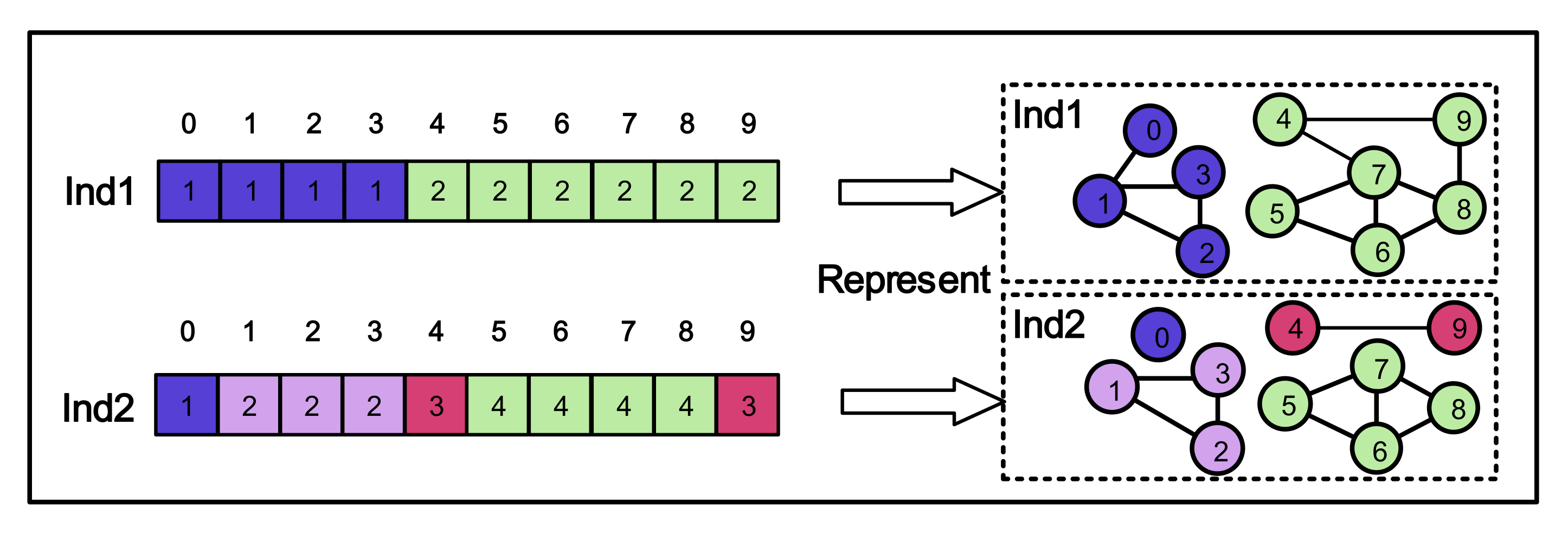
The solution encoding method is generally encoded as an individual that uses the LAR method [1,20]. Each solution is represented as an n-dimensional integer vector $X_j$. The i-th dimensional value $x_i$ of the solution $X_j$ is denoted as the neighbor node of the node $n_i$. Such an encoding scheme often results in a low-quality initialization, which slows down the convergence of the population evolution. Therefore, we propose a promising solution representation to improve the problems encountered above in Figure 1. As shown in Figure 1, node $n_i$ and node $n_j$ will belong to the same community if $x_i$ and $x_j$ have the same value. Nodes in different colors indicate that the nodes do not belong to the same communities. The i-th dimensional value $x_i$ of the solution $X_j$ is denoted as the label of the community in which node $n_i$ is located.

Figure 1. Two examples of solution representation.

3.3. Gray Wolf Optimization with a Novel Initialization and Two Improved Stages (NIGWO)

3.3.1. The Framework of NIGWO

In the GWO, the behavior of the elite gray wolves increases the global search ability and the diversity of the population. However, the GWO still suffers from the problems of being prone to local optima and slow convergence. Hence, the proposed NIGWO makes three significant improvements to the standard GWO algorithm, the framework of which is shown in Figure 2. The first improvement is a fast elite population initialization strategy to greatly accelerate the convergence speed of population evolution. Secondly, an improved hunting prey stage to share the excellent structure of the first three optimal solutions $\alpha ,\beta ,\delta$ of the contemporary population to improve other gray wolf individuals $\omega$ is presented. Thirdly, a multi-scales mutation strategy is proposed in the encircling prey stage to further improve search capability and increase the diversity of the gray wolf population. The specific NIGWO pseudocode is shown in Algorithm 1.

Algorithm 1: NIGWO

Input: $G,pop,p_{mu},MaxIter$ Output: The optimal individuals  1: Initialize the gray wolf population $X=[X_1,X_2,\dots ,X_{pop}]$ according to the fast elite population Initialization  2: Calculate the fitness of each gray wolf  3: $t\leftarrow 0$  4: while$t<MaxIter$do  5:     Get $X^{\prime }=[X_{\alpha },X_{\beta },X_{\delta },X_{\omega }]$ by sorting the population X  6:     Get $elite$ = $[X_{\alpha },X_{\beta },X_{\delta }]$ by X  7:     while $2<i<pop$ do  8:        Hunting operation by $elite$ for gray wolf individual $\omega$  9:     end while 10:    Execute a multi-scales mutation strategy 11:    t ← t + 1 12: end while 13: Return $X_{\alpha }$

Figure 2. The framework of the NIGWO.

3.3.2. Fast Elite Population Initialization

Two strategies are utilized to improve the quality and diversity of the initial population.

The first solutions are generated as the adjacent node-based initialization method [37]. In this initialization method, individual nodes are encoded using the neighboring node, which is selected randomly from the current node; then, the current node and its neighboring node are aggregated in the same community by decoding.

The second solutions are composed of solutions obtained by a fast elite initialization method. First, in the elite structure phase, a motif-based strategy is presented to find the elite structure of the community. Moreover, in the fast sorting phase, the remaining nodes are quickly sorted and labeled according to the existing substructures.

In the elite structure phase, our methods obtain sub-stable structures to decrease the search space by merging motifs structures. An example of the elite structure phase is presented in Figure 3. The sub-stable structures are the different set of motifs that is the stable structure in the community. Their definitions are given as follows:

Figure 3. The elite structure phase. (a) A graph structure of the network. (b) Generate motifs according to Defition 1. (c) Calculate sub-stable structure by Defition 2. (d) Nodes that have not yet been aggregated. (e) Preliminary division of the network.

Definition 1

(Motifs). Network motifs are dense and interconnected subgraphs occurring in complex networks at significantly higher numbers than those in randomized networks [23]. In this paper, only the three-node motifs are calculated, since the computation complexity of the three-node motifs is relatively low. In our work, a motif is defined as $G_{solid}$. Let $G_{solid}$ be a triple $(x,y,z)$ where $x,y,z$ are three nodes of G and $x,y\in G.adj\left[z\right]$, then $G_{solid}$ is a motif. It is the basis of the sub-stable community.

Definition 2

(Sub-stable community). A sub-stable community $G_{sec\_solid}$ is a community composed of two motifs, and the intersection between two motifs is greater than 1. It can be formalized as $G_{sec\_solid}=G_{solid1}\cup G_{solid2},s.t.G_{solid1}\cap G_{solid2}>1$. $G_{solid1}$ and $G_{solid2}$ are represented as the motifs.

In Figure 3, the initial graph network first generates three motifs and merges them based on Definition 2. The network is initially divided by the above process. In the next phase, these nodes $n_0$, $n_4$ and $n_9$ of the undivided community are divided into communities.

In the fast sorting phase, the remaining nodes are sorted and divided into communities according to the obtained elite structure. Inspired by the fast clustering algorithm (FCA) [21], a series of operations are defined on the graph of the community, and we extracted several features from it. The nodes are ordered according to a set of features by utilizing mathematical operations on the graph. Set the number of remaining nodes is q. The effect matrix $E=\{E_i\mid i=0,1,\cdots ,q\}$. We calculate the priority of these nodes by $E_i$ as follows:

$$\begin{array}{l}{E}_i=\frac{S_i}{{\sum }_{j=1}^n{K}_j\times S_j}\\ K_j=\left\{\begin{array}{c}\hfill 0,if{m}_d(i,j)=0\hfill \\ \hfill 1,if{m}_d(i,j)\ne 0\hfill \end{array}\right.\end{array}$$

(4)

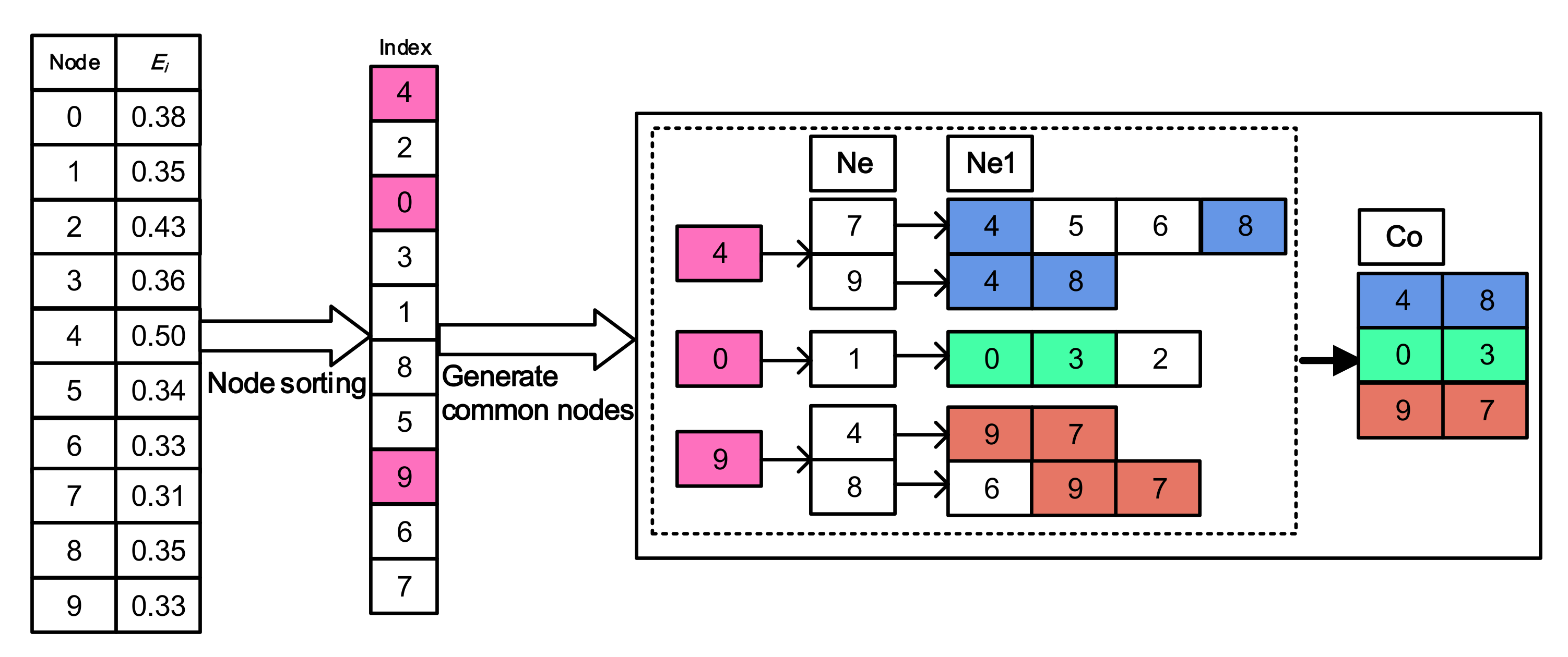
where the sum matrix S is an $n\times 1$ matrix, and the value of each row represents the sum $S_i$ of the degree of the adjacent nodes of the node $i\in [0,n)$, $m_d$ denotes the neighborhood degree matrix. The effect matrix E is an $n\times 1$ matrix. It is important to note that the largest $E_i$ is for a node that has not yet been aggregated and the clustering process of the remaining nodes starts with this node. Let $n_i$ and $n_j$ denote two nodes in the graph so that an edge between $n_i$ and $n_j$ indicates the existing dependency between them. We cluster nodes that have not yet been aggregated by performing some operations on the dependence matrix $m_d$ and extracting several features from it. The node importance array $index$ is obtained in descending order according to the effect matrix E, and the aggregation of the remaining nodes is completed by $index$. If each node is adjacent to the previous elite sub-community, it will be merged into this community; otherwise, it will be assigned by the label of the neighbor node. As shown in Figure 4, the nodes are sorted by $E_i$ to obtain the processing order, and then, their quadratic neighboring nodes are found to obtain corresponding communities $Co$.

Figure 4. The fast sorting phase. Ne (Ne1) represents the neighbor nodes of the previous nodes. Co represents the neighbor nodes shared by the previous nodes.

Finally, the uninitialized nodes will be divided into communities based on the elite substructure, and the $Co$ values obtained from the above two phases are shown in Figure 5. Nodes $n_4$, $n_0$, and $n_9$ will be divided into the communities where nodes $n_8$, $n_3$, and $n_7$ are located, respectively. The pseudocode of the initialization method is shown in Algorithm 2.

Algorithm 2: Fast elite population Initialization

Input: $G,pop$ Output: Population X  1: Find motifs of G by Definition 1  2: Get sub-stable communities by Definition 2  3: Get effect matrix E by Equation (4)  4: Get node sorted array $index$ according to the effect matrix E  5: $i\leftarrow 0$  6: while$i<pop/2$do  7:    Select sub-stable communities to update node label of $X_i$  8:    $z\leftarrow$ nodes without labels according to the order of $index$.  9:    $j\leftarrow 0$ 10:   while j is less than the length of z do 11:      Get the corresponding node y by $z\left[j\right]$ 12:      $k\leftarrow 0$ 13:      while k is less than the length of $Ns\left(y\right)$ do 14:         $set=Ns\left(Ns\right(y\left)\right[k\left]\right)\cap Ns\left(y\right)$ 15:         if $set$ not $null$ then 16:             Update the label of node z to the label of $set$ 17:         else 18:             Update the label of node z by the label of the neighbor node 19:         end if 20:         k←$k+1$ 21:      end while 22:      j←$j+1$ 23:    end while 24:    i←$i+1$ 25: end while 26: $ii\leftarrow pop/2$ 27: while$ii<pop$do 28:    Initialize the gray wolf individual by the adjacent node-based method 29: end while 30: Return population X

Figure 5. Population initialization based on the elite structure phase and the fast sorting phase. (a) Preliminary division of the network. (b) Initial partition of the network.

3.3.3. Improved Hunting Stage

Based on the characteristics of the CD problem, we design a new hunting stage to improve the hunting behavior of the gray wolf. In the classical GWO, each individual explores prey locations through elite wolfs (the leaders $\alpha$, $\beta$, and $\delta$), and the position of the prey is calculated according to Equation (2). However, this strategy cannot be directly applied to the CD, since CD is a discrete space search optimization problem. We leverage the elite substructure among the population to reduce the search space and improve search efficiency. Therefore, we take the intersection of $\alpha$, $\beta$, and $\delta$ as the prey position, and then the rest of the individuals update their positions according to the prey position. In this way, a good substructure among the elite solutions is obtained. Specifically, the intersection of $\alpha$, $\beta$, and $\delta$ is shown as follows:

$$subc=\left\{cs\right|cs\in (C_{\alpha }\cap C_{\beta }\cap C_{\delta })\}$$

Note that $C_{\alpha },C_{\beta }$, and $C_{\delta }$ are the communities set of $\alpha$, $\beta$, and $\delta$, respectively. The $cs$ represents the common subset of $C_{\alpha },C_{\beta }$, and $C_{\delta }$. We perform the intersection operation on the communities of $C_{\alpha },C_{\beta }$, and $C_{\delta }$. If the intersection of $\alpha$, $\beta$, and $\delta$ is empty, we select another gray wolf to replace $\omega$ until their intersection is not empty.

The new solution is obtained by updating the old solution with $subc$. Specifically, by randomly selecting a node i from $subc$, the other nodes in $subc$ are assigned the same community as node i. The updating process is given as follows:

$$x_j^{t+1}=\left\{\begin{array}{l}{x}_i^t,if(i,j)\in subc\\ x_j^t,else\end{array}\right.$$

In this way, the elite substructure is fused into the community structure of the old solution and is effectively used to improve the search efficiency.

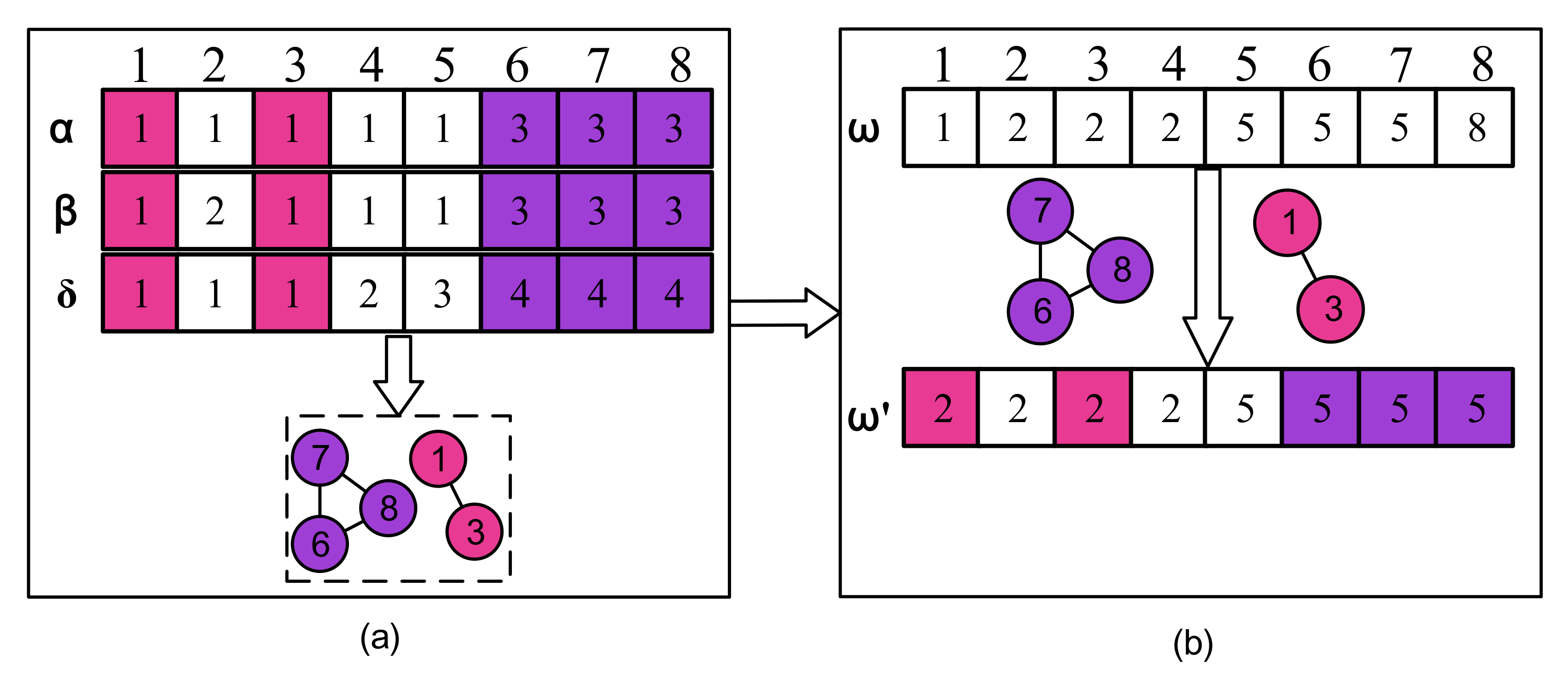
To further illustrate the improved hunting stage, we use an example to show the main idea of the improved hunting stage in Figure 6. The $subc$ generation process is given in Figure 6a. The $\alpha$, $\beta$, and $\delta$ are decoded separately to obtain the community sets. There, the high-quality network subsets are obtained as $subc$ among the three elite individuals. In Figure 6a, subc is {1, 3} and {6, 7, 8} as it the intersect of the $C_{\alpha },C_{\beta }$, and $C_{\delta }$. Then, in Figure 6b, the good substructure of $subc$ has remained in the new individual. Thus, the search space is greatly reduced by moving non-elite individuals closer to elite individuals and maintaining quality subsets of the community in the improved hunting phase.

Figure 6. The improved hunting stage. (a) is the generation process of $subc$, and (b) is the process by which $\omega$ wolf hunt for prey based on $subc$.

3.3.4. Improved Encircling Stage

Encircling prey behavior is essentially a random method-based mutation behavior from fast to slow. Therefore, we propose multi-scales mutation strategies to improve the quality of solutions and increase the diversity of the wolf population in the encircling stage. Boundary nodes and sub-community are utilized to mutate the individual on different scales.

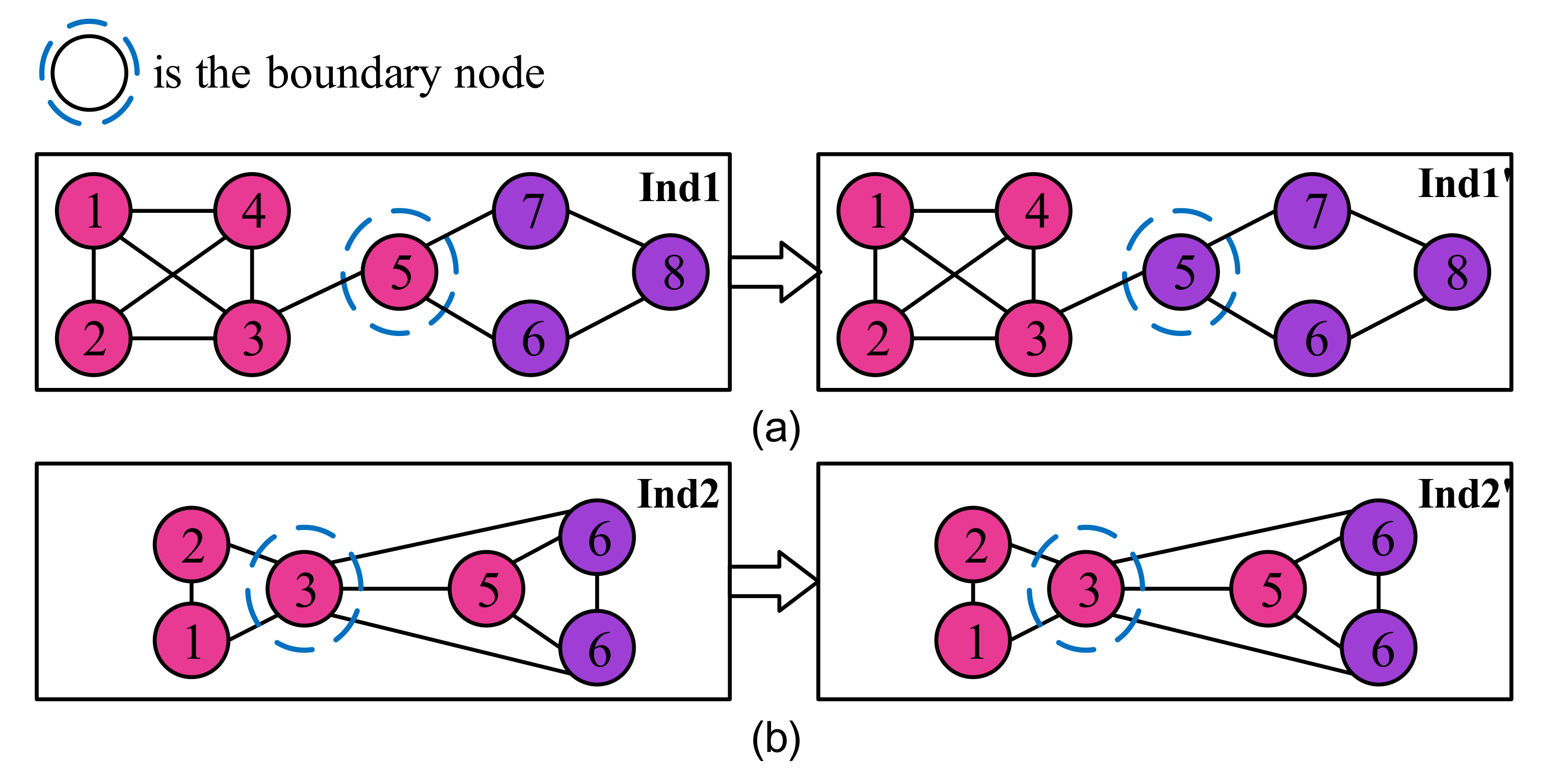
Firstly, the boundary nodes are selected to mutate as Liu et al. proposed the DECS algorithm to utilize the number of edges that boundary nodes to different communities to mutate and got a better performance [22]. However, the boundary node mutation process in DECS will not necessarily improve the performance of the CD when the two communities connected to the boundary node are complex. For example, the boundary node mutation process is shown in Figure 7. It shows that after the mutation of boundary node 5, the modularity value varies from 0.2149 to 0.3926. This improves the performance of the CD to a certain extent. However, in another case, as shown in Figure 7b, the initial value of modularity is 0.1667, and the value of modularity after boundary node mutation is 0.1235.

Figure 7. Boundary node mutation in DECS. (a) The performance of Ind1 has been improved. (b) The performance of Ind2 has been degraded.

The detailed definition of a boundary node can be found in [22]. We have improved the judgment conditions for mutation in the community mutation strategy. We adopt the Q calculation method of EP-WOCD [20], which defines the Q value from the perspective of the community. Different from his study, we propose a $\Delta Q$ method for boundary node mutation and improve the calculation method of the change value of Q. The derivation of the simplified formula for the change value of Q is as shown in Equation (5).

$$\begin{array}{l}\Delta Q=Q_{latter}-Q_{former}\\ \hspace{1em} ={\displaystyle \sum _{c=1}^k}[\frac{l_{cl}}{m}-{(\frac{d_{cl}}{2m})}^2]-{\displaystyle \sum _{c=1}^k}[\frac{l_{cf}}{m}-{(\frac{d_{cf}}{2m})}^2]\end{array}$$

(5)

where $l_{cl}$ and $l_{cf}$ represent the total number of community edge connections after and before the boundary nodes mutation, respectively. Since $l_c$ and $d_c$ are not changed except for the two involved communities in the process of mutation, the calculation of $\Delta Q$ can be updated as:

$$\Delta Q=(\Delta l_1+\Delta l_2)/m-(\Delta d_1^2+\Delta d_2^2)/4m^2$$

where $\Delta l_1$ ($\Delta l_2$) and $\Delta d_1^2$ ($\Delta d_2^2$) represent the changes in the number of edges and squares of the sum of nodes degree in the community, respectively. The change of the Q value is affected by the number of edges of two communities. Some large-scale networks have hundreds or thousands of communities. The time calculation cost can be greatly reduced by $\Delta Q>0$ since $\Delta Q>0$ only needs to calculate two communities. When $\Delta Q>0$, the boundary node mutation is executed. Otherwise, it will remain unchanged. In the above example, we only need to calculate the change value of $l_k$ and the change value of $d_k$ square of the two communities. Therefore, we effectively improve the search efficiency and save the computation assumption by mutating boundary nodes through $\Delta Q$.

Secondly, the community mutation operator is shown in Figure 8, in which the label of one community is changed to the label of its neighbor community. It can be observed that there exist a lot of small communities after the initialization. These small communities can be effectively integrated by the community mutation operator. In this way, the community mutation can be effectively utilized to improve the performance of the individuals.

Figure 8. Community mutation.

Obviously, these nodes in {9, 1, 0} in Figure 8 belongs to the same community. In the process of community mutation, these three nodes will find the community closest to them for community mutation and assimilate into the same community.

3.4. Time Complexity Analysis

As shown in Algorithm 1, the gray wolf population initialization is executed $pop$ times in step 1. The network has n nodes, so the total time is $O(n\times pop)$ in population initialization. During steps 7–8, the hunting operation is performed for all gray wolf individuals except $\alpha ,\beta ,\delta$, since the encoding time of each individual is $O\left(n\right)$. Therefore, the total time cost of the improved encircling stage is $O(MaxIter\times (n\times (pop-3)\left)\right)$. In the improved encircling stage, which contains boundary node variation and community variation, the time for boundary node variation is mainly spent on finding boundary nodes, so the time complexity is $O\left(n\right)$. For community variation, the time complexity is $O(k+n+pop)$ because the number of communities in the network is k and the number of nodes in each community needs to be counted. The time complexity of the improved encircling stage is $O(MaxIter\times (k+2n+pop\left)\right)$ in step 10. Therefore, this total time complexity is $O(pop\times n+MaxIter\times (n(pop-1)+k+pop\left)\right)$.

4. Experiment and Evaluation

4.1. Datasets and Comparison Algorithms

To evaluate the effectiveness of NIGWO in community discovery, we test and experiment on 11 different scales and different fields of real datasets and two groups of artificial networks. The artificial network used in the experiment is the LFR benchmark network [44]. The LFR network can generate the network to be tested in the investigation according to any configuration parameters. Eleven real data sets are used for experiments from Network Data (http://www-personal.umich.edu/~mejn/netdata/, accessed on 21 July 2022), SNAP [45], LINQS (https://linqs.soe.ucsc.edu/data/, accessed on 11 June 2022). There are six datasets: Karate, Football, Dolphins, Polbooks, Lesmis, and Netscience from Network Data. For the two networks, CA-GrQc and CA-HepTh in SNAP, it is used to evaluate the performance of the large-scale complex networks under different algorithms. The network datasets in LINQS are Cora, Citeseer, and Pebmud, respectively. The details of the eleven real data are in Table 2, where $d_{max}$ represents the maximum degree of nodes in the dataset, and $d_{ave}$ represents the average degree of nodes, which takes an approximate integer value by rounding down.

Table 2. The details of 11 networks.

Dataset	n	m	${\mathit{d}}_{\mathit{max}}$	${\mathit{d}}_{\mathit{ave}}$
Karate	34	78	17	4
Football	115	613	12	10
Dolphon	62	159	12	5
Polbooks	105	441	25	8
Lesmis	77	254	36	6
Netscience	1589	2742	34	3
CA-GrQc	5242	14,496	81	5
CA-HepTh	9877	25,998	65	5
Cora	2708	5429	168	3
Citeseer	3312	4732	99	3
Pebmud	19,717	44,327	171	4

The performance of NIGWO is compared with four popular EA-based CD algorithms for complex networks, namely, Meta-LPAM+ [19], DMFWA [14], EP-WOCD [20], RMOEA [1]; and five popular NMF-based CD algorithms namely NSED [46], BigClam [47], MNMF [13], DANMF [12], and NMFGAAE [11]; and other CD algorithms, namely, DeepWalk [48], and LPA [34]. NMFGAAE is also a method based on NMF, which is a combination of the graph neural network and NMF-based method. The details of the eleven algorithms are in Table 3.

Table 3. The details of 11 algorithms.

Algorithm	Types	Reference
Meta-LPAM+	Swarm intelligence	[19]
DMFWA	Swarm intelligence	[14]
EP-WOCD	Swarm intelligence	[20]
RMOEA	Swarm intelligence	[1]
NSED	NMF	[46]
BigClam	NMF	[47]
MNMF	NMF	[13]
DANMF	NMF	[12]
NMFGAAE	NMF	[11]
DeepWalk	Other	[48]
LPA	Other	[34]

4.2. Parameters Setting and Evaluation Metrics

The value of parameters has a great influence on the performance of the algorithm. There are three parameters that need to be specified before the NIGWO is executed, namely, the initial population size $pop$, the number of iterations $MaxIter$, and the mutation probability $p_{mu}$. In order to facilitate the comparison and analysis of the experiments, the parameters of the evolutionary algorithms used in the experiments are set uniformly and compared. The parameter settings are shown in Table 4. Significantly, our algorithm does not need to adjust the parameters, and there is no randomness. We set the population size of DMFWA, EP-WOCD, RMOEA, and NIGWO to 100 and the number of iterations to 40 uniformly. The other parameters are set by default in the original paper.

Table 4. Parameters setting of the compared evolutionary algorithms.

Algorithm	$\mathit{pop}$	$\mathit{MaxIter}$	${\mathit{p}}_{\mathit{mu}}$	Reference
Meta-LPAm+	1	100	—	[19]
DMFWA	100	40	—	[14]
EP-WOCD	100	40	0.3	[20]
RMOEA	100	40	0.1	[1]
NIGWO	100	40	0.4	[ours]

“—” means that there is no corresponding parameter.

For real-world networks and synthetic networks, we use modularity and NMI as evaluation metrics, respectively. Modularity is defined in Equation (3). The NMI is defined as follows.

$$NMI(A,B)=\frac{-2{\sum }_{i=1}^{k_A}{\sum }_{j=1}^{k_B}{N}_{ij}log\frac{n·N_{ij}}{N_i{N}_j}}{{\sum }_{i=1}^{k_A}{N}_{i}log\frac{N_i}{n}+{\sum }_{j=1}^{k_B}{N}_{j}log\frac{N_j}{n}}$$

where A is the network division obtained through CD, and B is the real division of the network. $k_A$ and $k_B$ represent the number of communities of A and B, respectively. n represents the dimension of the complex network, that is, the number of nodes. $N_{ij}$ represents the number of nodes that co-occur in community i and j. $N_i$ and $N_j$ are the number of nodes in community i and j, respectively.

4.3. Experiments on Real-World Networks

For real-world network datasets, some datasets have labels and some datasets have no labels. We make the modularity comparison of the twelve algorithms listed above for real-world networks, and the result is shown in Table 5.

Table 5. Modularity values comparison between algorithms.

Networks	Meta-LPAm+	DMFWA	NSED	BigClam	DeepWalk	LPA	MNMF	DANMF	EP-WOCD	RMOEA	NMFGAAE	NIGWO
Karate	0.4198	0.4038	0.2181	0.3005	0.2448	0.3049	0.2321	0.3644	0.4198	0.3875	—	0.4198
Football	0.6044	0.6041	0.4877	0.2177	0.5543	0.5297	0.5706	0.6091	0.6023	0.6041	—	0.6044
Dolphins	0.5174	0.5013	0.3134	0.3481	0.0192	0.4934	0.3627	0.5175	0.5242	0.5264	—	0.5275
Polbooks	0.5027	0.5081	0.3763	0.2238	0.3714	0.4519	0.3845	0.3986	0.5269	0.5264	—	0.5271
Lesmis	0.5562	0.5349	0.4538	0.3862	—	0.5171	0.4719	0.4246	0.5596	0.4398	—	0.5491
Netscience	0.9478	0.9124	0.7196	0.8285	—	0.8916	0.6864	0.7944	0.9183	0.9521	—	0.9548
Cora	—	—	0.6921	0.4713	0.6514	0.6275	0.7120	0.7129	0.6489	0.6636	0.7413	0.7535
Citeseer	—	—	0.5910	0.5802	0.4904	0.7002	0.6319	0.6524	0.6805	0.7454	0.7211	0.7693
CA-GrQc	—	—	0.3287	0.5052	—	0.7198	0.6329	0.6492	—	0.7962	—	0.7598
CA-HepTh	—	—	0.3775	0.3277	—	0.5472	0.5392	0.1417	—	0.4532	—	0.5257
Pebmud	—	—	0.3921	0.5317	0.3214	0.5073	0.5119	0.5213	—	0.5068	0.5501	0.5389

In Table 5, it can seem that our algorithm has more obvious advantages than other algorithms. Especially on the Netscience network, NIGWO has better modularity than other algorithms. In these experiments, an interesting phenomenon is that the LPA algorithm performs poorly on small data. However, as the network size increases, LPA will instead perform well. For example, our method shows good competitiveness in Netscience, Citeseer, Ca-HepTh, and Pubmed networks. One of the main problems in CD is the inability of the existing algorithms to maintain consistently good performance as the network scales. However, the results of experiments clearly show that NIGWO can maintain a good community detection performance on datasets of different scales.

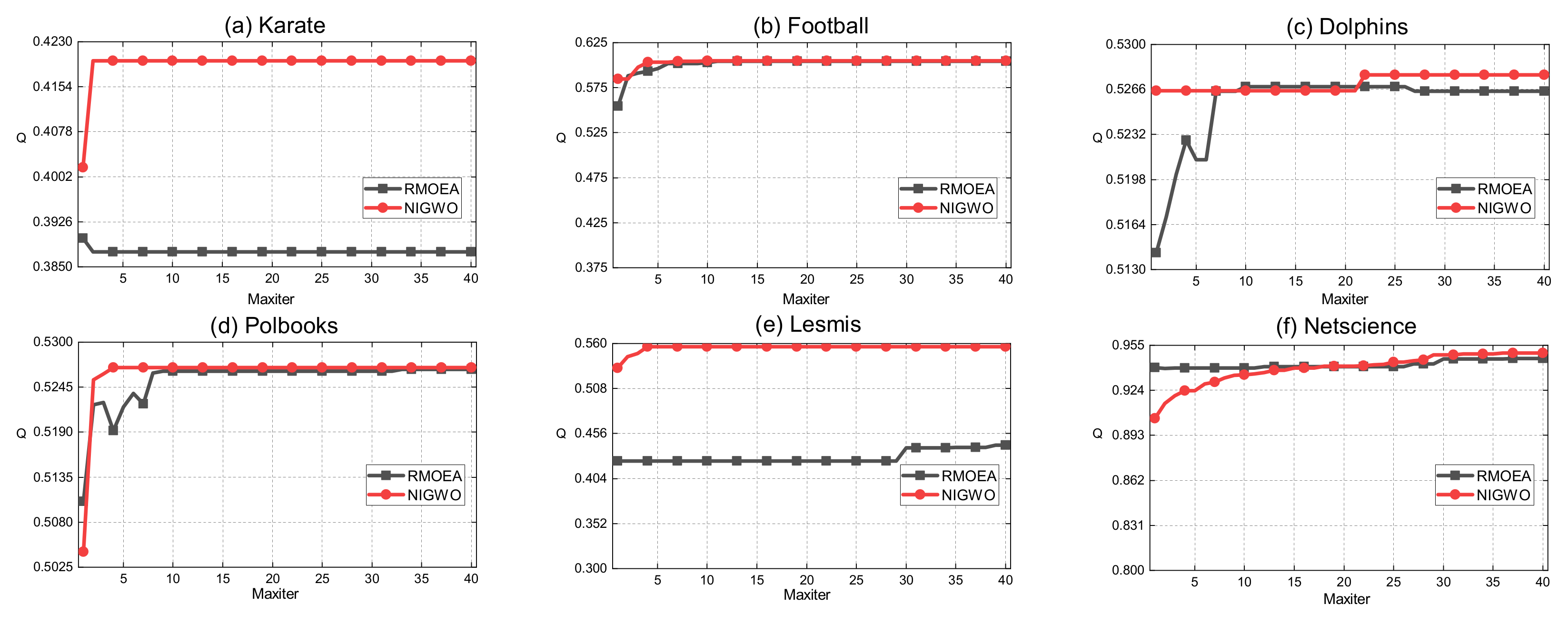
To evaluate the convergence of the experiments, we perform the population evolution comparison on two algorithms (RMOEA and NIGWO) on six networks. Figure 9 shows the changes in the modularity of the six datasets under the population evolution of the two algorithms. Obviously, NIGWO has better performance and faster convergence in most networks, such as Karate, Dolphins, Polbooks, Netscience, and Lesmis networks.

Figure 9. Modularity based on population evolution.

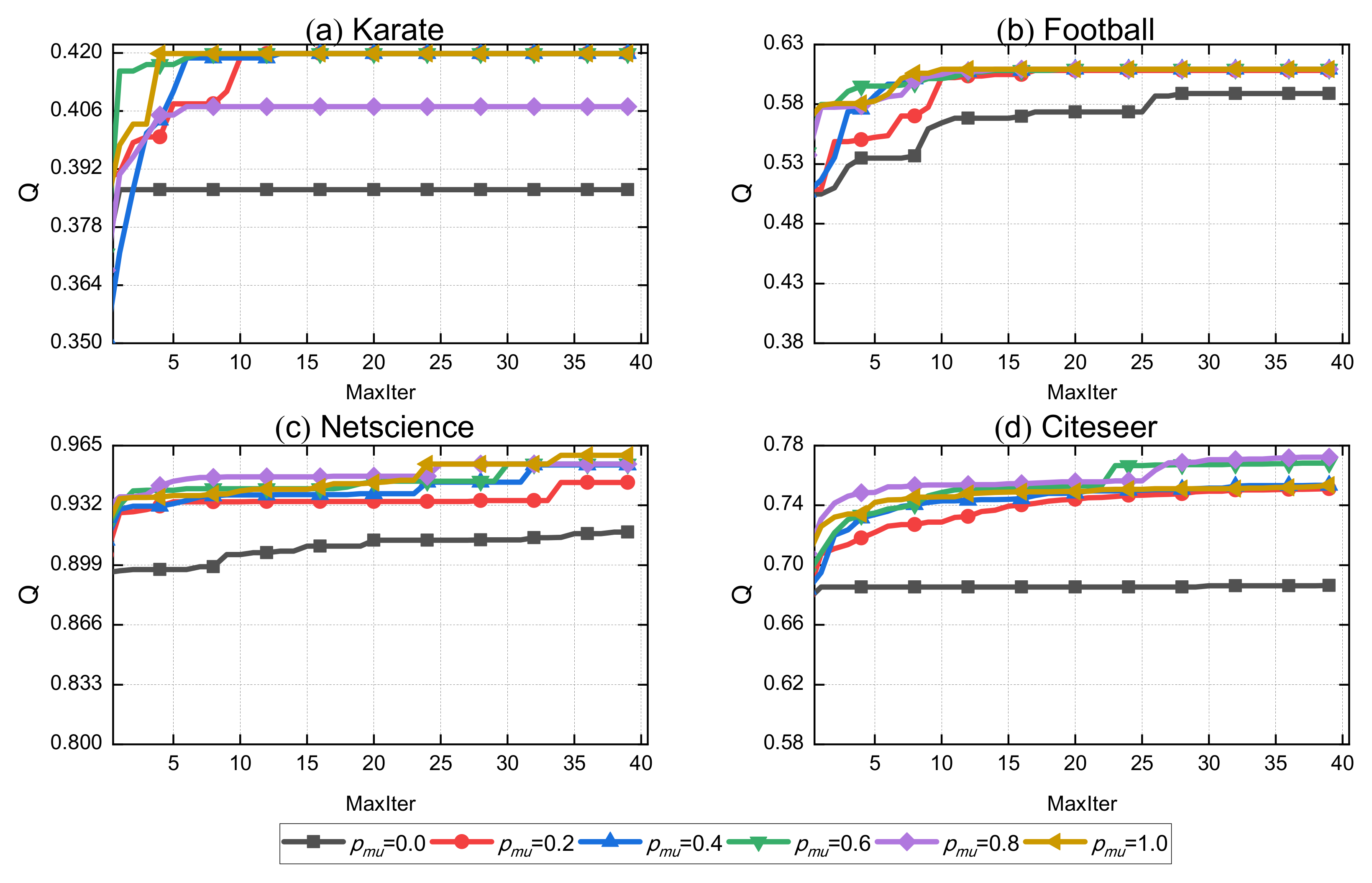
To verify the validity of our proposed multi-scales mutation, we performed an experimental comparison of different $p_{mu}$ values in Figure 10. It can be clearly observed that the performance decreases a lot when no mutation strategy is implemented. After implementing the mutation strategy, the performance is improved to a great extent. At the same time, we can find that the performance increases with a higher mutation probability, and the convergence is also incremental. The convergence and community detection performance reach the optimum when $p_{mu}$ is at 1. However, due to the time cost, the performance of NIGWO is finally close to the optimal value at 0.4. Therefore, we set the probability value of $p_{mu}$ at 0.4 to balance time and performance. In the last citeseer data, the value of modularity decreases when the variation probability becomes 1. This is because of the inability to jump out of the local optimum due to excessive variation, which is the reason why we finally set the variation probability to 0.4.

Figure 10. Comparison of Q in different $p_{mu}$ with four real-world networks.

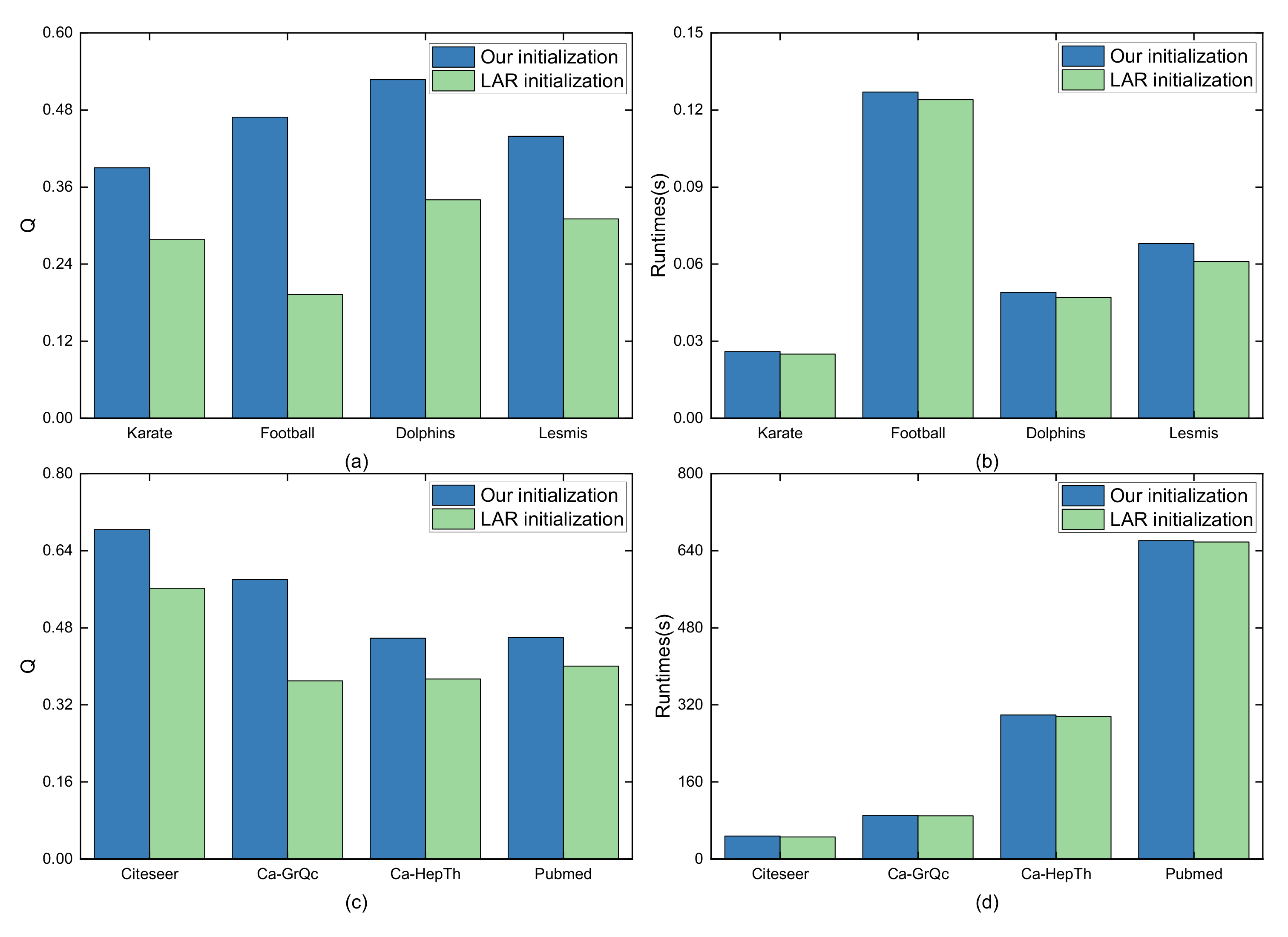
To verify the validity of our initialization, we performed a comparison of the improved LAR initialization method of EP-WOCD (i.e., LAR Initialization here for convenience) in Figure 11. Since the time difference between small and large data is large, the comparison with small and large datasets separately is executed. We perform a comparison of Q and time consumption for four small datasets. The result is shown in Figure 11a,b. For the four small datasets Karate, Football, Dolphins, and Lesmis, our initialization method has significantly better performance on the small datasets and is only a small difference in time cost from LAR initialization. Similarly, on the large datasets Citeseer, Ca-GrQc, Ca-HeppTh, and Pubmed, although the performance of the LAR-based initialization method is improved, the improvement is limited. As Figure 11c,d show, our initialization method achieves better performance at about a similar time cost. In addition, higher quality initialized populations tend to allow the evolutionary algorithm to reach the optimal solution faster, speeding up the convergence of community detection.

Figure 11. Comparison of different initialization methods. (a) Comparison of Q for four small datasets. (b) Comparison of time for four small datasets. (c) Comparison of Q for four big datasets. (d) Comparison of time for four big datasets.

4.4. Experiments on LFR Networks

In our work, two groups of LFR networks are used to further evaluate NIGWO. The first group consists of networks with 500 nodes and the mixing parameter $\mu$ from 0.1 to 0.8, $\mu$ is a fraction that each node shares with the other nodes of the network. In addition, 1-$\mu$ is that each node shares a fraction of its links with the other nodes of its community [44]. The average degree $d_{ave}=5$, the maximum degree $d_{max}=15$, the minimum community size $C_{min}=20$, the maximum community size $C_{max}=50$, the exponents of the power law distribution of node degrees ${\tau }_1=2$, and the power law exponent community sizes distribution ${\tau }_2=1$; the second group is these networks where the number of nodes is from 1000 to 5000, and the $\mu$ value is fixed to 0.3, the minimum community $C_{min}=50$, the maximum community size $C_{max}=100$, the exponents of the power law distribution of node degrees ${\tau }_1=2$, the power law exponent community sizes distribution ${\tau }_2=1$, the average degree $d_{ave}=4$, and the maximum degree $d_{max}=15$. A comparative experiment is completed for the second group with NMI, and the experimental results are shown in Table 6.

Table 6. NMI comparison for LFR with different nodes.

Nodes	NSED	BigClam	DeepWalk	LPA	MNMF	DANMF	EP-WOCD	RMOEA	NMFGAAE	NIGWO
1000	0.20	0.03	0.19	0.47	0.18	0.41	0.32	0.36	0.46	0.50
2000	0.30	0.14	0.19	0.55	0.28	0.47	0.33	0.44	0.52	0.57
3000	0.34	0.20	0.19	0.56	0.24	0.53	0.33	0.45	0.58	0.59
4000	0.38	0.22	0.18	0.60	0.26	0.56	0.32	0.48	0.60	0.62
5000	0.39	0.22	0.18	0.62	0.40	0.58	0.32	0.50	0.61	0.63

In Table 6, we can clearly see that our algorithm outperforms other algorithms at any time. In the worst case, our algorithm also improves the performance by 5.1%. Overall, the performance of NIGWO has been greatly improved compared to other algorithms.

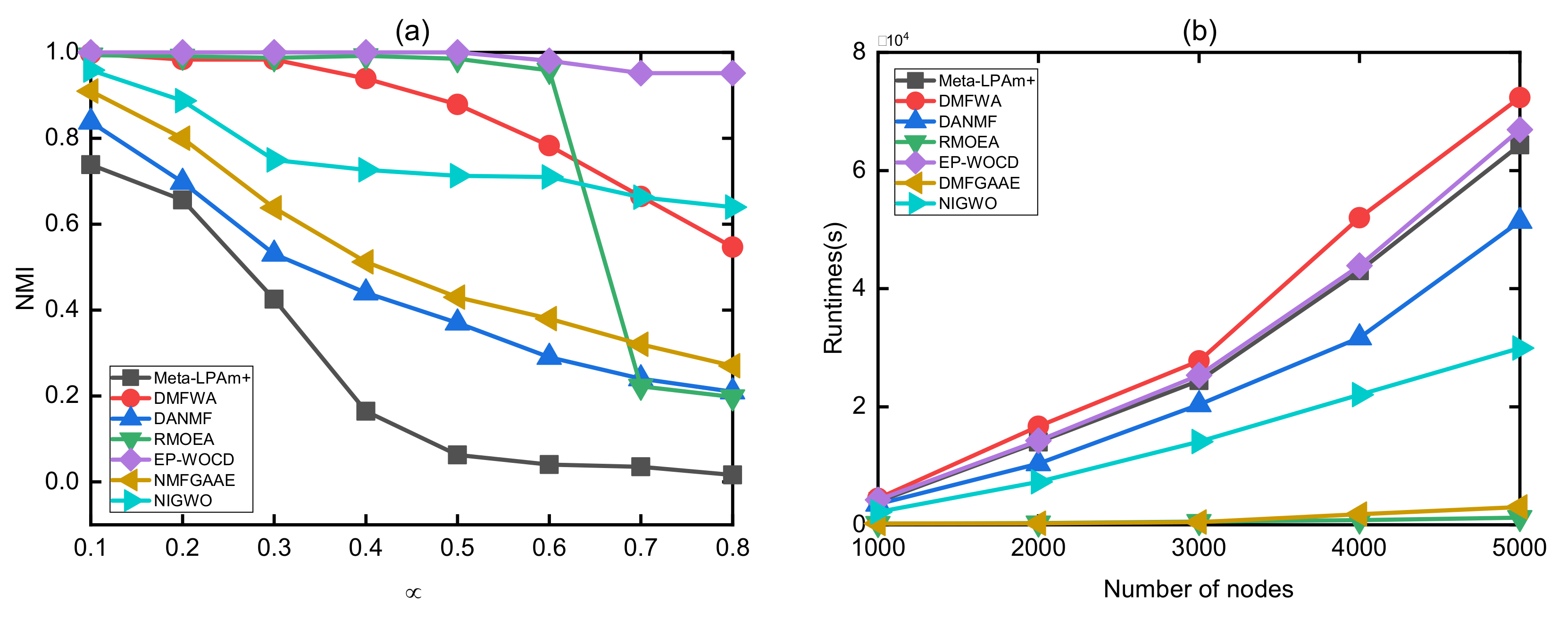
Then, we compare the accuracy of six algorithms in the first group of the LFR which have different $\mu$, and the experimental results are shown in Figure 12a. As shown in Figure 12a, the NMI value shows a decreasing trend with the increase of $\mu$. The increase of $\mu$ will make the community structure more complex. In addition, the results of NIGWO have well NMI when compared with the other algorithms. As the value of $\mu$ increases, the NMI of RMOEA and DMFWA decreases sharply, while our proposed NIGWO method can be clearly seen to be decreasing slowly. When $\mu >$ 0.4, our method decreases smoothly and obviously has a more stable performance than Meta-LPAm+, DMFWA, and RMOEA.

Figure 12. Comparison on LFR networks. (a) Comparison of NMI at different $\mu$. (b) Comparison of time at different number of nodes.

We further compare our experiments with other excellent experiments in terms of time. The results of experiments are obviously much faster than Meta-LPAm+, DMFWA, EP-WOCD, and DANMF in terms of operating efficiency, and they are only slower than RMOEA and NMFGAAE. RMOEA algorithmically treats a good community structure as a node, which leads to a large-scale reduction of large-scale complex networks, thereby greatly improving operating efficiency, so it has a very fast operating speed. This sacrifices some performance in exchange for time efficiency. In the end, our algorithm achieves a balance in terms of time complexity and performance.

As can be seen in Figure 12b, for the second group of the LFR, our algorithm is slightly longer in time complexity than the current excellent algorithm RMOEA. However, with the expansion of the network size, our algorithm requires more time, because the more complex the network, the more information is hidden, which requires a longer time for mining. We sacrifice time on complex networks, which brings a great improvement in modularity and NMI on complex networks.

As analyzed above, the advantage of our algorithm’s performance is that it can reach the optimal NMI and modularity on most networks, and it can achieve a high NMI and modularity. Our method also performs well on both small and large datasets.

4.5. Visualization of NIGWO

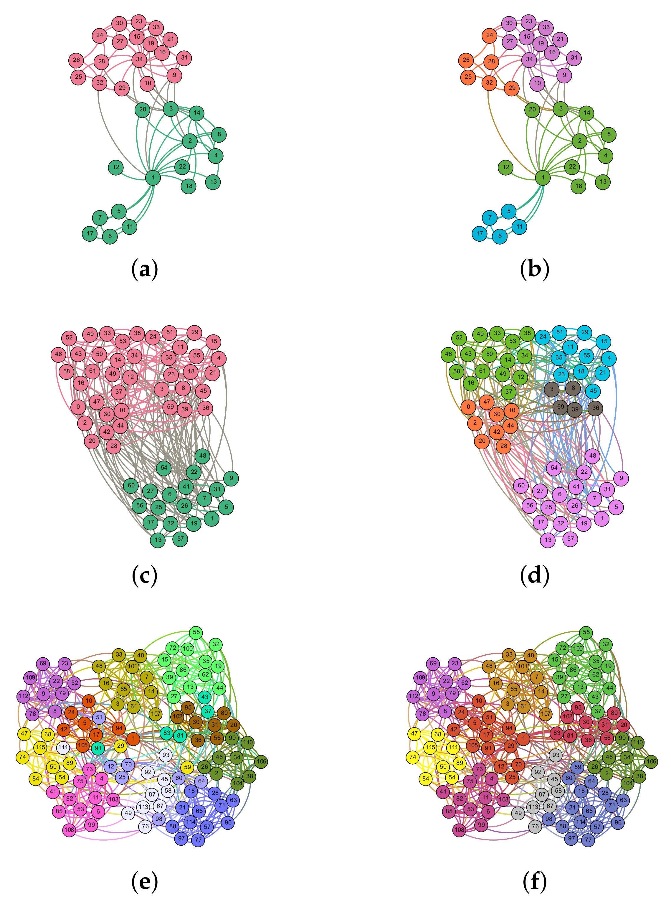
We apply our proposed method to divide the three datasets with real labels into communities and visualize them. The three datasets are the Karate network, Dolphins network, Football network.

The visualization is shown in Figure 13. In this figure, the communities detected by our algorithm are not consistent with the original communities, because some of the accuracies are sacrificed while improving the robustness of the network. For example, in the Karate dataset, the Q value of Karate is only 0.3715, but the detection performance is improved to 0.4198 by our algorithm. Similarly, in the Football network, the Q value of the real community is only 0.554, but the Q value reaches 0.6046 by NIGWO. In the Dolphins network, the Q value under the real community is only 0.3735, while the Q value can reach 0.5285 after NIGWO.

Figure 13. Community structure of three networks. (a) Ground-truth communities of Karate network. (b) Communities detected by NIGWO of Karate network. (c) Ground-truth communities of Dolphins network. (d) Communities detected by NIGWO of Dolphins network. (e) Ground-truth communities of Football network. (f) Communities detected by NIGWO of Football network.

5. Conclusions

In the paper, we proposed a new algorithm NIGWO to solve CD problems. In NIGWO, we designed a novel initialization method and two improved operators of GWO. The initialization method greatly enhances the quality of the initial population and improves the convergence speed by defining sub-stable communities from the network structure and diffusing the neighborhood according to various features of nodes. During this evolution, the improved hunting stage and improved encircling stage are further designed to enhance the efficiency of the algorithm and ensure the quality of the results on small and large datasets. The two operators have improved the search performance of GWO by utilizing the characteristics of the good substructure and boundary node.

Experiments show that our algorithm obtains higher-quality solutions for detecting communities in large-scale complex networks. Therefore, the increasingly complex network can be solved efficiently, and communities in social networks, biological networks, protein molecular networks, etc. can be detected effectively. A good initialization method is crucial to the swarm intelligence algorithm. We will design an effective initialization strategy to further improve the quality of the initialization population. At the same time, the features of the local community and paralleled framework can be investigated to reduce the dimension of complex networks and reduce time consumption in large-scale network problems.

References

1. Zhang, X.; Zhou, K.; Pan, H.; Zhang, L.; Zeng, X.; Jin, Y. A network reduction-based multiobjective evolutionary algorithm for community detection in large-scale complex networks. IEEE Trans. Cybern. 2018, 50, 703–716. [Google Scholar] [CrossRef] [PubMed]
2. Karataş, A.; Şahin, S. Application areas of community detection: A review. In Proceedings of the 2018 International Congress on Big Data, Deep Learning and Fighting Cyber Terrorism (IBIGDELFT), Ankara, Turkey, 3–4 December 2018; pp. 65–70. [Google Scholar]
3. Qing, Q.; Jian, C.; Yancen, L. The Evolution of Software Ecosystem in GitHub. J. Comput. Res. Dev. 2020, 57, 513. [Google Scholar]
4. Yang, T.; Xie, J.; Zhao, J.; Dong, H.; Hu, K. Design and Application of Chinese Medicine Association Discovery Algorithm Based on Association Network and Hierarchical Clustering. Mod. Tradit. Chin. Med. Mater. Med.—Sci. Technol. 2020, 22, 1962–1968. [Google Scholar]
5. Lu, D.D. Leader-Based Community Detection Algorithm in Attributed Networks. IEEE Access 2021, 9, 119666–119674. [Google Scholar] [CrossRef]
6. Liu, Q.; Su, Y.; Peng, Q.; Chen, K.; Lu, Y. An Overlapping Community Detection Algorithm for Label Propagation Based on Node Influence. In Proceedings of the 2021 3rd International Conference on Advances in Computer Technology, Information Science and Communication (CTISC), Shanghai, China, 23–25 April 2021; pp. 183–187. [Google Scholar] [CrossRef]
7. Roghani, H.; Bouyer, A. A Fast Local Balanced Label Diffusion Algorithm for Community Detection in Social Networks. IEEE Trans. Knowl. Data Eng. 2022. [Google Scholar] [CrossRef]
8. Huang, J.; Hou, Y.; Li, Y. Efficient community detection algorithm based on higher-order structures in complex networks. Chaos Interdiscip. J. Nonlinear Sci. 2020, 30, 023114. [Google Scholar] [CrossRef]
9. Li, C.; Tang, Y.; Tang, Z.; Cao, J.; Zhang, Y. Motif-based embedding label propagation algorithm for community detection. Int. J. Intell. Syst. 2022, 37, 1880–1902. [Google Scholar] [CrossRef]
10. Li, P.Z.; Huang, L.; Wang, C.D.; Lai, J.H.; Huang, D. Community detection by motif-aware label propagation. ACM Trans. Knowl. Discov. Data (TKDD) 2020, 14, 1–19. [Google Scholar] [CrossRef]
11. He, C.; Zheng, Y.; Fei, X.; Li, H.; Hu, Z.; Tang, Y. Boosting nonnegative matrix factorization based community detection with graph attention auto-encoder. IEEE Trans. Big Data 2021, 8, 968–981. [Google Scholar] [CrossRef]
12. Ye, F.; Chen, C.; Zheng, Z. Deep autoencoder-like nonnegative matrix factorization for community detection. In Proceedings of the 27th ACM International Conference on Information and Knowledge Management, Torino, Italy, 22–26 October 2018; pp. 1393–1402. [Google Scholar]
13. Wang, X.; Cui, P.; Wang, J.; Pei, J.; Zhu, W.; Yang, S. Community preserving network embedding. In Proceedings of the Thirty-First AAAI Conference on Artificial Intelligence, San Francisco, CA, USA, 4–9 February 2017. [Google Scholar]
14. Guendouz, M.; Amine, A.; Hamou, R.M. A discrete modified fireworks algorithm for community detection in complex networks. Appl. Intell. 2017, 46, 373–385. [Google Scholar] [CrossRef]
15. Liu, F.; Xue, S.; Wu, J.; Zhou, C.; Hu, W.; Paris, C.; Nepal, S.; Yang, J.; Yu, P.S. Deep learning for community detection: Progress, challenges and opportunities. arXiv 2020, arXiv:2005.08225. [Google Scholar]
16. Wang, P.; Kong, B.; Bao, C.; Zhou, L.; Wang, C. Community Detection Based On Graph Neural Network. In Proceedings of the 2021 6th International Conference on Intelligent Computing and Signal Processing (ICSP), Xi’an, China, 9–11 April 2021; pp. 89–93. [Google Scholar] [CrossRef]
17. Su, X.; Xue, S.; Liu, F.; Wu, J.; Yang, J.; Zhou, C.; Hu, W.; Paris, C.; Nepal, S.; Jin, D.; et al. A Comprehensive Survey on Community Detection With Deep Learning. IEEE Trans. Neural Netw. Learn. Syst. 2022, 1–21. [Google Scholar] [CrossRef] [PubMed]
18. Kang, Y.; Pu, B.; Kou, Y.; Yang, Y.; Chen, J.; Muhammad, K.; Yang, P.; Xu, L.; Hijji, M. A deep graph network with multiple similarity for user clustering in human–computer interaction. ACM Trans. Multimed. Comput. Commun. Appl. (TOMM), 2022; just accepted. [Google Scholar] [CrossRef]
19. Le, B.D.; Shen, H.; Nguyen, H.; Falkner, N. Improved network community detection using meta-heuristic based label propagation. Appl. Intell. 2019, 49, 1451–1466. [Google Scholar] [CrossRef]
20. Feng, Y.; Chen, H.; Li, T.; Luo, C. A novel community detection method based on whale optimization algorithm with evolutionary population. Appl. Intell. 2020, 50, 2503–2522. [Google Scholar] [CrossRef]
21. Teymourian, N.; Izadkhah, H.; Isazadeh, A. A fast clustering algorithm for modularization of large-scale software systems. IEEE Trans. Softw. Eng. 2020, 48, 1451–1462. [Google Scholar] [CrossRef]
22. Liu, F.; Wu, J.; Xue, S.; Zhou, C.; Yang, J.; Sheng, Q. Detecting the evolving community structure in dynamic social networks. World Wide Web 2020, 23, 715–733. [Google Scholar] [CrossRef]
23. Milo, R.; Shen-Orr, S.; Itzkovitz, S.; Kashtan, N.; Chklovskii, D.; Alon, U. Network motifs: Simple building blocks of complex networks. Science 2002, 298, 824–827. [Google Scholar] [CrossRef]
24. Tang, J.; Liu, G.; Pan, Q. A review on representative swarm intelligence algorithms for solving optimization problems: Applications and trends. IEEE/CAA J. Autom. Sin. 2021, 8, 1627–1643. [Google Scholar] [CrossRef]
25. Lou, S.; Wu, P.; Guo, L.; Duan, Y.; Zhang, X.; Gao, J. Sparse principal component analysis using particle swarm optimization. J. Chem. Eng. Jpn. 2020, 53, 327–336. [Google Scholar] [CrossRef]
26. Ramirez-Figueroa, J.A.; Martin-Barreiro, C.; Nieto-Librero, A.B.; Leiva, V.; Galindo-Villardón, M.P. A new principal component analysis by particle swarm optimization with an environmental application for data science. Stoch. Environ. Res. Risk Assess. 2021, 35, 1969–1984. [Google Scholar] [CrossRef]
27. Li, T.; Shi, J.; Deng, W.; Hu, Z. Pyramid particle swarm optimization with novel strategies of competition and cooperation. Appl. Soft Comput. 2022, 121, 108731. [Google Scholar] [CrossRef]
28. Bas, E.; Egrioglu, E.; Kolemen, E. Training simple recurrent deep artificial neural network for forecasting using particle swarm optimization. Granul. Comput. 2022, 7, 411–420. [Google Scholar] [CrossRef]
29. Cai, Q.; Gong, M.; Shen, B.; Ma, L.; Jiao, L. Discrete particle swarm optimization for identifying community structures in signed social networks. Neural Netw. 2014, 58, 4–13. [Google Scholar] [CrossRef] [PubMed]
30. Ahmed, K.; Hafez, A.I.; Hassanien, A.E. A discrete krill herd optimization algorithm for community detection. In Proceedings of the 2015 11th International Computer Engineering Conference (ICENCO), Cairo, Egypt, 29–30 December 2015; pp. 297–302. [Google Scholar]
31. Ma, T.; Xia, Z. A community detection algorithm based on local double rings and fireworks algorithm. In Proceedings of the International Conference on Intelligent Data Engineering and Automated Learning, Guilin, China, 30 October–1 November 2017; Springer: Cham, Switzerland, 2017; pp. 129–135. [Google Scholar]
32. Zhang, Y.; Liu, Y.; Li, J.; Zhu, J.; Yang, C.; Yang, W.; Wen, C. WOCDA: A whale optimization based community detection algorithm. Phys. A Stat. Mech. Its Appl. 2020, 539, 122937. [Google Scholar] [CrossRef]
33. Ma, T.; Xia, Z.; Yang, F. An ant colony random walk algorithm for overlapping community detection. In Proceedings of the International Conference on Intelligent Data Engineering and Automated Learning, Guilin, China, 30 October–1 November 2017; Springer: Cham, Switzerland, 2017; pp. 20–26. [Google Scholar]
34. Raghavan, U.N.; Albert, R.; Kumara, S. Near linear time algorithm to detect community structures in large-scale networks. Phys. Rev. E 2007, 76, 036106. [Google Scholar] [CrossRef]
35. Zeng, X.; Wang, W.; Chen, C.; Yen, G.G. A consensus community-based particle swarm optimization for dynamic community detection. IEEE Trans. Cybern. 2019, 50, 2502–2513. [Google Scholar] [CrossRef]
36. Handl, J.; Knowles, J. An evolutionary approach to multiobjective clustering. IEEE Trans. Evol. Comput. 2007, 11, 56–76. [Google Scholar] [CrossRef]
37. Wang, Y.J.; Song, J.X.; Sun, P. Research on Dynamic Community Detection Method Based on an Improved Pity Beetle Algorithm. IEEE Access 2022, 10, 43914–43933. [Google Scholar] [CrossRef]
38. Li, H.; Zhang, R.; Zhao, Z.; Liu, X. LPA-MNI: An Improved Label Propagation Algorithm Based on Modularity and Node Importance for Community Detection. Entropy 2021, 23, 497. [Google Scholar] [CrossRef]
39. Mirjalili, S.; Mirjalili, S.M.; Lewis, A. Grey wolf optimizer. Adv. Eng. Softw. 2014, 69, 46–61. [Google Scholar] [CrossRef]
40. Gupta, S.; Deep, K. Hybrid Grey Wolf Optimizer with Mutation Operator. In Soft Computing for Problem Solving; Advances in Intelligent Systems and Computing; Bansal, J., Das, K., Nagar, A., Deep, K., Ojha, A., Eds.; Springer: Singapore, 2019; Volume 817, pp. 961–968. [Google Scholar] [CrossRef]
41. Gupta, S.; Deep, K. Enhanced leadership-inspired grey wolf optimizer for global optimization problems. Eng. Comput. 2020, 36, 1777–1800. [Google Scholar] [CrossRef]
42. Liu, Y.; Sun, J.; Yu, H.; Wang, Y.; Zhou, X. An Improved Grey Wolf Optimizer Based on Differential Evolution and OTSU Algorithm. Appl. Sci. 2020, 10, 6343. [Google Scholar] [CrossRef]
43. Otsu, N. A threshold selection method from gray-level histograms. IEEE Trans. Syst. Man, Cybern. 1979, 9, 62–66. [Google Scholar] [CrossRef]
44. Lancichinetti, A.; Fortunato, S. Benchmarks for testing community detection algorithms on directed and weighted graphs with overlapping communities. Phys. Rev. E 2009, 80, 016118. [Google Scholar] [CrossRef]
45. Leskovec, J.; Krevl, A. SNAP Datasets: Stanford Large Network Dataset Collection. 2014. Available online: http://snap.stanford.edu/data (accessed on 7 May 2022).
46. Sun, B.J.; Shen, H.; Gao, J.; Ouyang, W.; Cheng, X. A non-negative symmetric encoder-decoder approach for community detection. In Proceedings of the 2017 ACM on Conference on Information and Knowledge Management, Singapore, 6–10 November 2017; pp. 597–606. [Google Scholar]
47. Yang, J.; Leskovec, J. Overlapping community detection at scale: A nonnegative matrix factorization approach. In Proceedings of the Sixth ACM International Conference on Web Search and Data Mining, Rome, Italy, 4–8 February 2013; pp. 587–596. [Google Scholar]
48. Perozzi, B.; Al-Rfou, R.; Skiena, S. Deepwalk: Online learning of social representations. In Proceedings of the 20th ACM SIGKDD International Conference on Knowledge Discovery and Data Mining, New York, NY, USA, 24–27 August 2014; pp. 701–710. [Google Scholar]
Publisher’s Note: MDPI stays neutral with regard to jurisdictional claims in published maps and institutional affiliations.
Article Metrics
Citations
Article Access Statistics
Multiple requests from the same IP address are counted as one view.