Article

A Revised Continuous Observation Length Model of Rough Contact without Adhesion

College of Mechanical and Electrical Engineering, Harbin Engineering University, Nantong Ave 145, Harbin 150001, China
*
Author to whom correspondence should be addressed.
Mathematics 2022, 10(20), 3764; https://doi.org/10.3390/math10203764
Submission received: 9 September 2022 / Revised: 9 October 2022 / Accepted: 10 October 2022 / Published: 12 October 2022

Abstract

:
The real contact area of rough surfaces has significant importance in many engineering applications, such as tribology, wear, lubrication and seals. A continuous observation length-dependent mechanic model of rough contact without adhesion is proposed, which assumes that the rough surface is divided into ideal subplanes. However, the model ignores the elastoplastic deformation of asperities, and the standard deviation of ideal subplanes’ heights is assumed to vary linearly with continuous observation length, which is not precise for all the surface fractal dimensions. In this work, a revised continuous observation length model is proposed with elastic, elastoplastic and fully plastic stages. The expressions of force and real contact areas are derived. For surfaces with different fractal dimensions, the quadratic polynomial, cubic polynomial and power relationships between standard deviation and observation length are proposed, respectively. In addition, the influences of the dimensionless observation length, fractal dimension and equivalent elastic modulus on the real contact areas in different contact stages are also analyzed. It can be concluded that the quadrate real contact area decreases as the dimensionless observation length decreases, which can be applied to the percolation theory for leak seal problems.

1. Introduction

The dimensions of these deviations and the surface topography vary in a big range from macro (millimeter) to micro (nanometer) and even down to the level of interatomic distance. Consequently, the contact tends to be localized and incomplete when the two surfaces are engaged with each other at the beginning. The real contact area is of great importance in many engineering applications, such as structural adhesives, tribology, wear, lubrication, as well as seals.
Several theoretical methods were employed to deal with surface contact. An important pioneer in this field was Hertz, who developed a classic elastic contact model for both macroscopic and microscopic contact problems. A common critical criterion of plastic contacts was proposed by Tabor [1]. The pioneering work of the rough surface contact was contributed by Greenwood and Williamson, who proposed a single-length elastic contact model (GW model) for a rough surface based on Hertz’s theory and statistical method [2]. Whitehouse and Archar assumed that the curvature radius of the asperity is dependent on its height and proposed the WA model based on the GW model. The CEB model was also based on the GW model with the assumption that the volume of plastic deformation is conserved [3]. Xu et al. developed statistical models based on the GW model and extended the range of application of the classic models to the case of near complete contact [4]. Majumdar and Bhushan developed a very popular analytic method (MB model) for the contact problem of fractal rough surfaces, in which the real contact area was calculated using the two length-independent parameters: surface fractal dimension and fractal roughness [5]. Zhao et al. presented an elastoplastic model (ZMC model) and introduced a template function between the elastic and fully plastic models [6]. Liou and Lin modified the MB model with morphology parameters [7]. Kogut and Etsion subdivided the elastoplastic contact into two stages to improve accuracy [8]. Morag and Etsion presented an improved ME model concerning the relationship between the critical contact area and the critical load [9]. Yuan et al. applied Kogut and Etsion’s two-stage elastoplastic deformations to the MB model and observed the length dependency of the critical interference, the critical contact area and the critical load of the fractal single asperity [10]. Hanaor et al. applied a spline-assisted discretization method to the contact mechanics of two fractal surfaces, and an oblique contact of asperities was considered [11]. Pan et al. established the unloading fractal prediction model using the rough contact model results of the single asperity by Etsion [12]. Wen et al., proposed an analytical model of elastic–plastic contact for three-dimensional rough surfaces considering the interaction of asperities [13]. These single-length contact approaches have resolved a substantial number of rough contact problems, e.g., adhesive contact analysis [14], elastoplastic contact analysis [15,16], electrical conduction [17], partial slip behavior [18], contact stiffness [19,20,21,22] and unloading of contacting rough surfaces [23,24].
Persson developed a different theoretical model of the real contact area varying with the magnification [25]. Afferrante et al. presented an improved contact model based on Persson’s model [26]. The coalescence and elastic coupling between the contact regions were taken into account. Ciavarella suggested a simple closed-form approximate solution to the adhesive contact problem based on Persson’s model [27]. Guo et al., developed a magnification-based multi-asperity (MBMA) model by evolving magnification into the GW model, and the multilength nature of a rough surface was taken into account properly [28]. Liu et al., presented an observation length-dependent (OLD) model of rough contact without adhesion, which covered the shortage of the real contact area stops changing as the average stress reaches the plastic yield stress in the Perrson model [29]. Persson’s magnification offers a new way to solve a number of rough contact problems, e.g., the leak rate of sealing [30,31], the influence of surface roughness on hydrophobicity [32], adhesion [33,34] and friction [35,36,37].
However, the OLD model still had some disadvantages, such as ignoring the elastoplastic deformation stage of asperities, not using the dimensionless observation length parameter and assuming an inaccurate linear relationship between the standard deviation of the ideal subplanes’ heights and the continuous observation length, especially for some surface fractal dimensions. In this work, a revised continuous observation length model with elastic, elastoplastic and fully plastic stages is presented, and it is assumed that the standard deviation is a cubic polynomial with the continuous observation length. Moreover, quadratic polynomial, cubic polynomial and power equations are induced to describe the relationship between the standard deviation and the continuous observation scale more precisely. Furthermore, the influences of the surface fractal dimension and the equivalent elastic modulus on the relationship between the real contact areas and the dimensionless observation scale in various contact stages are discussed. Finally, the model is verified through a comparison with the Persson model and the OLD model.

2. Theoretical Framework

2.1. The OLD Model

The contact area is different when two contact surfaces are studied at different observation lengths. The two surfaces appear to be in complete contact at a large observation length because the surface roughness is neglected due to its small length. The incomplete contact emerges in reality with a small observation length, even in extremely tight contact conditions.
As the observation length decreases, the incomplete contact becomes gradual. While the observation length tends to a very small value (atomic length), the contact area of the two surfaces tends to zero [25].
Recently, Liu et al., proposed an observation length-dependent (OLD) mechanic model to calculate the real contact area for a frictionless contact between an elastic–perfectly plastic rough surface and a rigid plane [29]. In the model, the surface profile was determined by the WM function, and the contact of two rough surfaces can be idealized as a rigid plane pressed on a deformable rough surface, as shown in Figure 1a. The sample surface with the sample length L0 was regarded as a discrete surface composed of ideal subplanes with the observation length λ, λ0 < λ < L0, as shown in Figure 1b. The ideal subplanes were regarded as asperities of the same curvature radius at a certain observation length when the contact force and the real contact area were calculated, as shown in Figure 1c. Therefore, the contact of a rigid plane and a deformable rough surface can be idealized as the contact between a rigid plane and deformable ideal subplanes. The height of the asperity is the average height of the asperity at the observation length division plane. Assuming that the heights of the ideal subplanes follow the Gaussian distribution in all observation lengths, the standard deviation of the ideal subplane height can be obtained. To obtain the relationship between the observation length and standard deviation, a linear relationship was assumed (as shown in Section 2.1.1).
However, there are three problems in this model: (a) assuming that the standard deviation of the ideal subplane height varies linearly with successive observed lengths is not accurate for all the surface fractal dimensions; (b) no dimensionless parameters were used; (c) the model only investigated the elastic and plastic deformation of the asperities but ignored the elastic–plastic deformation. This leads to errors in solving the real contact area and contact force. To solve these problems, a revised continuous observation length model is presented.

2.1.1. The Standard Deviation

According to the multiscale characteristics of a rough surface, it is assumed that the rough surface is isotropic, and the W-M function can be used to define the surface profile [5,14]. The height of the surface profile z(x) is
z ( x ) = G ( D 1 ) n = n l γ ( 2 D ) n cos ( 2 π γ n x ) , 1 < D < 2 , γ > 1 ,
where D is the fractal dimension of the surface profile, and 1 < D < 2, G is the fractal roughness parameter of the surface; γn determines the frequency spectrum of the surface roughness, and γ ≥ 1.0. For most typical surfaces, γ = 1.5. nl is the minimum frequency index, and nl = logγ (1/L0).
As can be seen in Figure 1, the height of an arbitrary ideal subplane is
h ( λ ) = d ( λ ) + ω ,
where h(λ) is the height of the ideal subplane; ω is the contact deformation; and d(λ) is the distance between the reference plane and the rigid plane after contact. λ is the observation length.
The standard deviation of the ideal subplane is
σ ( λ ) = h ( x , λ ) = h 1 h ( x , λ ) = h i [ h ( x , λ ) h ¯ ( λ ) ] 2 ,
where x represents the coordinate of the ideal subplane; h(λ) is the average height of the ideal subplane.
Assuming that the height of the ideal subplane obeys the Gaussian distribution on all observation lengths, the probability density of ideal subplane height distribution at observation length λ is
f ( x , λ ) = 1 2 π σ ( λ ) e h 2 ( x , λ ) 2 σ 2 ( λ ) ,
where σ is the standard deviation of the ideal subplane height distribution, h(λ) = 0. In the OLD model, Liu et al. assume a linear relationship applies, and (λ) can be expressed as
σ ( λ ) = k λ + y 0 ,
where k is the linear fitting slope; y0 is the standard deviation of the surface profile at the minimum observation length.
It can be seen that the standard deviation was assumed to vary linearly with the observed lengths, which is not accurate. Additionally, the observation length is not dimensionless to eliminate the influence of sample length.

2.2. The Revised Continuous Observation Length Model

According to the OLD model, it is assumed that the rough surfaces are composed of ideal subplanes with the same observation length and asperity curvature radius, and every subplane obtains a specific height with regard to statistics. The multilength contact mechanics model of the rough surface is established based on the above assumptions.

2.2.1. The Standard Deviation

Surface profiles with various D and G, listed in Table 1, are used to calculate the standard deviation (λ) of the ideal subplane height using Equations (1) and (2).
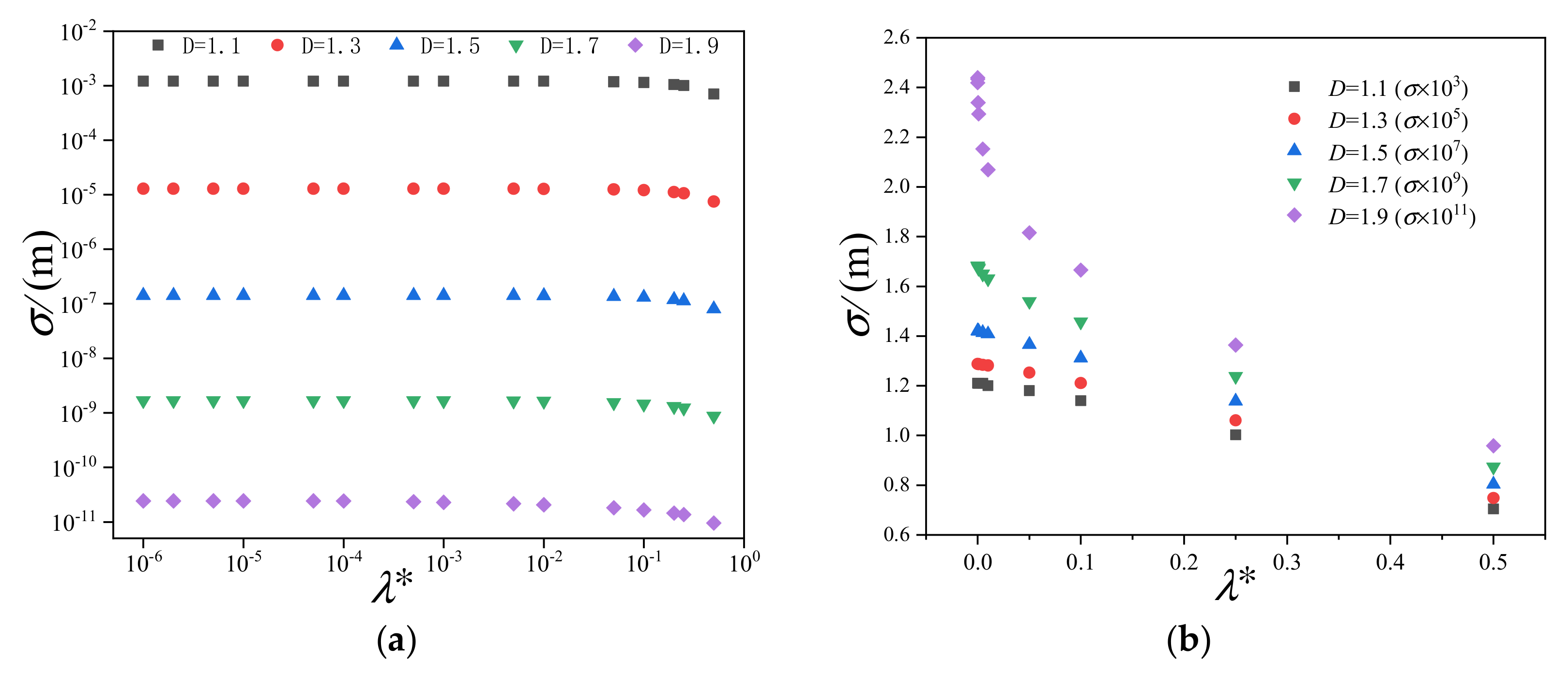
According to Equation (1), D has a significant effect on the height of the rough surface profile. To simplify the problem, it is assumed that the observation length λ is continuous. The variation of the standard deviation σ with λ* at different D is shown in Figure 2, where λ* is the dimensionless observation length (the observation scale) and λ* = λ/L0. The observation length is nondimensionalized to eliminate the influence of sampling length.
The surface profiles with various D, listed in Table 1, are used to calculate the standard deviation σ of the ideal subplane height. λmin is the minimum observation length. According to the W-M function, D has a significant effect on the height of the rough surface profile [38].
It can be seen from Figure 2a that σ increases monotonically with the decrease in λ*. Moreover, the σ of the surface with a larger D is smaller when the λ* is the same. It is obvious that different D has a great impact on the order of magnitude of σ. In order to facilitate observation, the standard deviation is magnified by a certain multiple, as shown in Figure 2b.
From Figure 2b, when D = 1.5, the relationship between λ* and σ is approximately linear. When D < 1.5, the rising rate of σ slows down at a small λ*. When D > 1.5, the rising rate speeds up. This is because the value of D has an influence on the variation relationship between σ and λ*. It can be seen from Equation (1) that z(x) is directly proportional to G(D−1), and z(x) becomes smaller as D becomes bigger. When the λ* is small, the change of z(x) is significant due to the increase in D. Therefore, the standard deviation σ also changes greatly, resulting in different rising rates.
After analyzing the calculation results under different D, the fitting is divided into two parts: D ≤ 1.5 and D > 1.5. The best fitting methods under different D are also different.
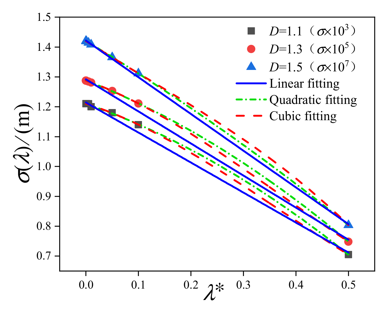
When D ≤ 1.5, linear fitting (σ = y0 + B1λ*), quadratic polynomial fitting (σ = y0 + B1λ* + B2λ*2) and cubic polynomial fitting (σ = y0 + B1λ* + B2λ*2 + B3λ*3) are adopted, respectively. The fitting curves of λ* and σ are shown in Figure 3. It can be seen that the linear fitting curves have a large deviation from the data points compared to the polynomial fitting curves. The quadratic fitting curves and the cubic fitting curves are more consistent with the data points. Thus, the polynomial fitting is better than the linear fitting.
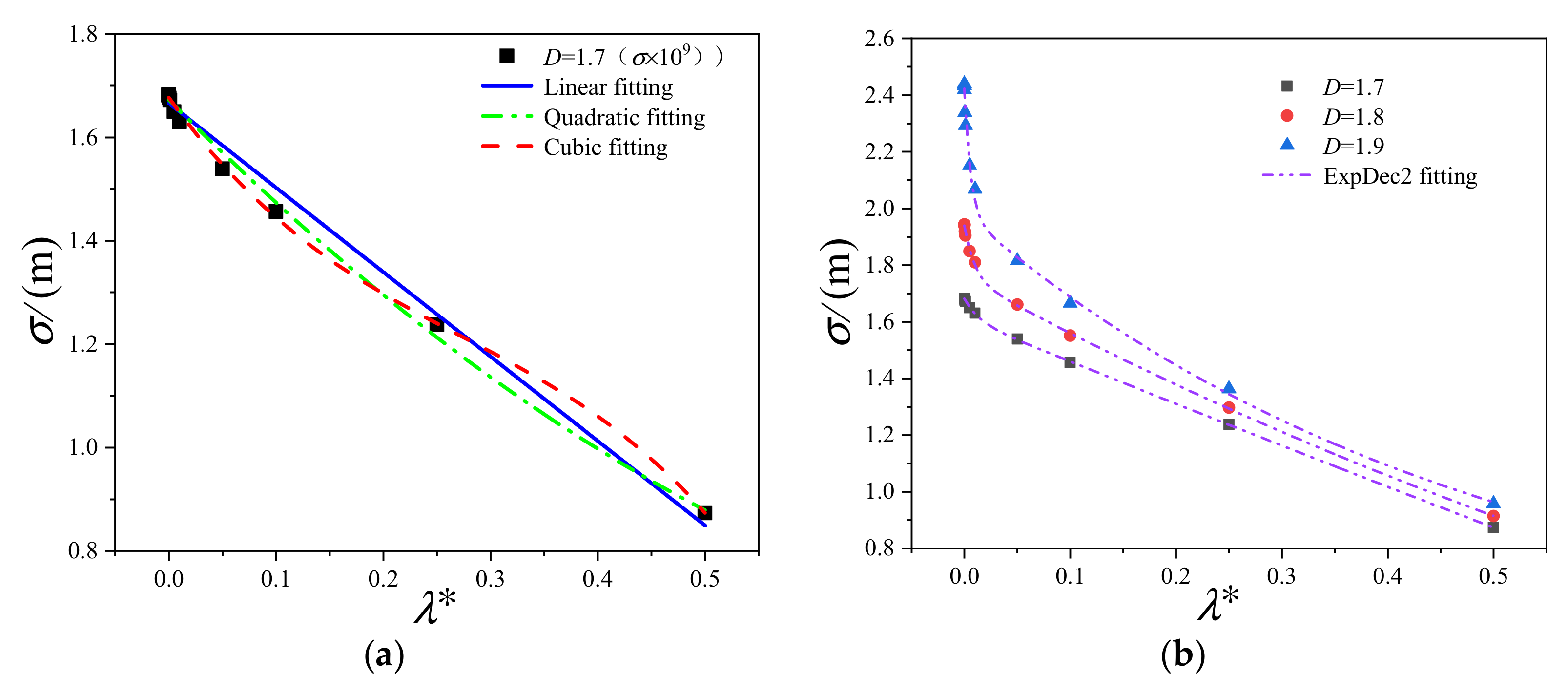
When D > 1.5, it can be seen from Figure 2b that the variation between λ* and σ is obvious. The other values of D, 1.7, 1.8 and 1.9, are taken for detailed analysis. At the small λ*, the rising rate of σ becomes much larger, so the cubic fitting relationship is no longer good. Finally, the ExpDec2 function (σ = y0 + B1 ex/A1 + B1 ex/A2) is used for fitting. The fitting curves of λ* and σ are shown in Figure 4.
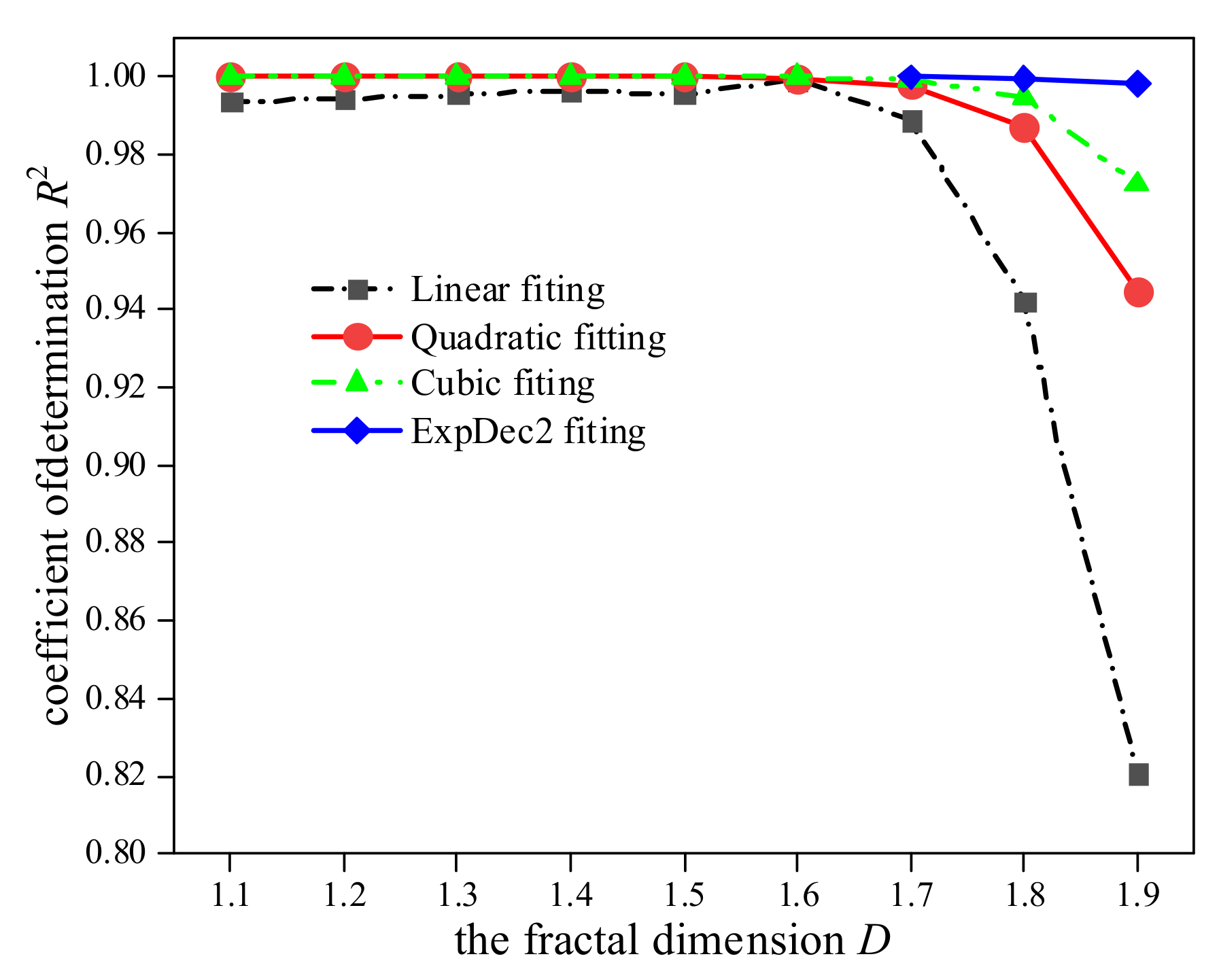
The coefficient of determination R2 is important to evaluate the fitting effect. The closer the value of R2 is to 1, the better the fit of the model. The relationship between R2 and D in different fitting methods is shown in Figure 5. It can be concluded that: (a) when D ≤ 1.5, the power fitting is not suitable; (b) when D ≤ 1.5, the R2 of all the three fitting methods is above 0.99, which is well fitted. Among the three methods, there is little difference between the two polynomial fitting methods, both of which are better than linear fitting, and the difference gradually decreases with the increase in D; (c) when D = 1.6, the R2 of the three fitting methods is basically the same. However, from the figure, the quadratic polynomial fitting is more in line with the requirements; (d) when D ≥ 1.7, the R2 of the linear fitting and polynomial fitting decreases with the increase in D. When D = 1.9, the R2 of the linear fitting, quadratic fitting and cubic fitting is 0.82, 0.94, 0.96, respectively. This indicates that the fitting is poor. In addition, the R2 of the ExpDec2 function fitting is bigger than 0.99, which is better than the other fitting methods.

2.2.2. Establishment of Contact Mechanics Model

The W-M function provides the asperity profile at any λ [38]:
z p ( λ ) = G D 1 λ 2 D cos ( π x λ ) , ( λ 2 x λ 2 ) ,
Therefore, the asperity curvature radius is
R ( λ ) = 1 + d z p / d x 2 3 / 2 d 2 z p / d x 2 x = 0 = λ D G D 1   π 2 ,
The critical contact depth ωe of the plastic contact is derived by Jackson based on Von Mises’ yield criterion, as shown below:
ω e = ( π K H 2 E ) 2 R = ( π K ϕ 2 ) 2 R ,
where K is the hardness coefficient related to the Poisson ratio ν of the material by K = 0.454 + 0.41 ν. H is the hardness of the softer material, H = 2.8σY, and σY is the yield strength. ϕ is the material property, ϕ = H/E. E is the equivalent modulus of Hertzian elasticity and equals
1 E = 1 ν 1 2 E 1 + 1 ν 2 2 E 2 ,
where E1, E2, ν1 and ν2 are the Young’s modulus and Poisson’s ratios of two contacting surfaces, respectively.

2.3. Contact Areas and Mechanics

At the macrolevel, the machined surface is a smooth surface, but it is a rough surface at the microlevel. Therefore, the contact between the two surfaces, which are assembled together, is actually the contact between asperities. According to the ideal subplane asperity deformation, there are three contact states: elastic, elastoplastic and plastic deformation. The elastic contact state indicates that the ideal subplanes are fully in elastic contact. The plastic contact state indicates that the plastic contact dominates, and the elastic contact is extremely small. The elastoplastic deformation stage is in between and is divided into two stages. In the OLD model, the elastoplastic deformation was ignored, which makes the results inaccurate. Kogut and Etsion used the finite element method to analyze the mechanical behavior of elastoplastic contact of a single spherical asperity [8]. When 0 < ω < ωe, the asperity is at elastic deformation, and the ideal subplane height of elastic deformation should be d(λ) < h(x, λ) ≤ d(λ) + ωe. When ωe < ω < 6ωe, it is the first stage of elastoplastic deformation, and the height should be d(x, λ) + ωe < h(x, λ) ≤ d(x, λ) + 6ωe. When 6ωe < ω < 110ωe, it is the second stage of elastoplastic deformation, and the height should be d(x, λ) + 6ωe < h(x, λ)≤ d(x, λ) + 110ωe. In addition, when ω > 110 ωe, the contact is completely plastic.

2.3.1. The Areas in Different Stages

The real area Ar of contact is
A r ( λ ) = L 0 2 d ( λ ) f ( h , λ ) d h ,
where d(λ) is the separation of the rigid plane and the reference plane of the deformable rough surface at the observation length λ.
The real elastic contact area Are is
A re = L 0 2 d ( λ ) ω e + d ( λ ) f ( h , λ ) d h
During the first stage of elastoplastic contact, the contact area Arep1 is
A rep 1 = L 0 2 ω e + d ( λ ) 6 ω e + d ( λ ) f ( h , λ ) d h
During the second stage of elastoplastic contact, the contact area Arep2 is
A rep 2 = L 0 2 6 ω e + d ( λ ) 110 ω e + d ( λ ) f ( h , λ ) d h
The real plastic contact area Arp is
A rp = L 0 2 110 ω e + d ( λ ) f ( h , λ ) d h
The dimensionless areas in different stages can be, respectively, written as
A re = A re A 0 = d ( λ ) ω e + d ( λ ) f ( h , λ ) d h ,
A rep 1 = A rep 1 A 0 = ω e + d ( λ ) 6 ω e + d ( λ ) f ( h , λ ) d h ,
A rep 2 = A rep 1 A 0 = ω e + d ( λ ) 6 ω e + d ( λ ) f ( h , λ ) d h ,
A rp = A rp A 0 = 110 ω e + d ( λ ) f ( h , λ ) d h ,
where A0 is the nominal area, A0 = L02.
The total dimensionless contact area Ar* is obtained by accumulating the different stages’ contributions. Hence, from Equations (14)–(17)
A r = A re + A rep 1 + A rep 2 + A rp

2.3.2. The Relationship between F and ωe of Single Asperity

The relationship between the contact of a single asperity and the critical contact depth is [8]
F re = 4 3 E R 1 2 ω 3 2 ,
( F rep 1 F ec ) 1 = 1.03 ( ω ω e ) 1.425 ,
( F rep 2 F ec ) 2 = 1.40 ( ω ω e ) 1.263 ,
F rp = 2 π R ω H ,
where ωe is the critical contact depth; Fre, Frep1, Frep2 and Frp are the contact forces of a single asperity in four stages; Fec is the critical contact force of the elastic contact. The critical contact force is
F ec = 4 3 E R 1 2 ω e 3 2

2.3.3. The Contact Force of the Surfaces in Different Stages

The surface contact forces consist of elastic, elastoplastic and plastic parts and can be described as
P r = P re + P rep 1 + P rep 2 + P rp ,
where Pre, Prep and Prp are the elastic, elastoplastic and plastic contact forces with the observation length λ, which can be calculated as the sum of forces in different stages of asperities.
P re = 4 E A 0 3 λ 2 R ( λ ) 1 2 d ( λ ) ω e + d ( λ ) [ h ( x , λ ) d ( λ ) ] 3 2 2 π σ ( λ ) e h 2 ( x , λ ) 2 σ 2 ( λ ) d h ,
P rep 1 = 1.373 E 0.85 R ( λ ) 0.575 ( π K H 2 ) 0.15 A 0 λ 2 ω e + d ( λ ) 6 ω e + d ( λ ) [ h ( x , λ ) d ( λ ) ] 1.425 2 π σ ( λ ) e h 2 ( x , λ ) 2 σ 2 ( λ ) d h ,
P rep 2 = 1.867 E 0.526 R ( λ ) 0.737 ( π K H 2 ) 0.474 A 0 λ 2 6 ω e + d ( λ ) 110 ω e + d ( λ ) [ h ( x , λ ) d ( λ ) ] 1.263 2 π σ ( λ ) e h 2 ( x , λ ) 2 σ 2 ( λ ) d h ,
P rp = 2 π H R ( λ ) A 0 λ 2 110 ω e + d ( λ ) [ h ( x , λ ) d ( λ ) ] 2 π σ ( λ ) e h 2 ( x , λ ) 2 σ 2 ( λ ) d h
The dimensionless contact force P N with EA0 is
P N ( λ ) = P N ( λ ) E A 0
The mean contact stress σ0 is
σ 0 = P r E A 0
The dimensionless contact forces are
P re = 4 R ( λ ) 1 2 3 λ 2 d ( λ ) ω e + d ( λ ) [ h ( x , λ ) d ( λ ) ] 3 2 2 π σ ( λ ) e h 2 ( x , λ ) 2 σ 2 ( λ ) d h ,
P rep 1 = 1.373 ( π K 2 ) 0.15 R ( λ ) 0.575 λ 2 ω e + d ( λ ) 6 ω e + d ( λ ) [ h ( x , λ ) d ( λ ) ] 1.425 2 π σ ( λ ) e h 2 ( x , λ ) 2 σ 2 ( λ ) d h ,
P rep 2 = 2 π H R ( λ ) A 0 λ 2 110 ω e + d ( λ ) [ h ( x , λ ) d ( λ ) ] 2 π σ ( λ ) e h 2 ( x , λ ) 2 σ 2 ( λ ) d h ,
P rp = 2 π R ( λ ) 1 λ 2 110 ω e + d ( λ ) [ h ( x , λ ) d ( λ ) ] 2 π σ ( λ ) e h 2 ( x , λ ) 2 σ 2 ( λ ) d h .
The total dimensionless contact force is
P c = P re + P rep 1 + P rep 2 + P rp
The surface contact force PN and the nominal area A0 are usually known for a certain contact system and will not change with the observation length λ. The separation d(λ) at any observation length can be solved by the numerical method. Consequently, the real contact area, elastic contact area and plastic contact area can be calculated with d(λ).

3. Numerical Results and Discussion

In order to study multilength contact characters, the following common parameters are selected: the surface fractal dimension D = 1.3, 1.4 and 1.5; the equivalent modulus of Hertzien E = 50 GP, 75 GPa and 100 GPa; the fractal roughness parameter G = 1 × 10⁻¹² m; the Poisson’s ratio ν = 0.3 and the yield strength σY = 345 MPa. The mean contact stress σ0 is 10 MPa. By numerical analysis in Python, the changing rules between the contact area and λ* are obtained. The numerical analysis is based on the above equation through circular iterations and judgments.

3.1. Surface Fractal Parameters

3.1.1. The Influence of the Fractal Dimension

The fractal surface profiles obtained by Equation (5) with G = 1 × 10⁻¹² m and D = 1.3, 1.4, 1.5 are plotted in Figure 6. After abundant and repetitive simulations, we found out that a high value of D results in more surface details.
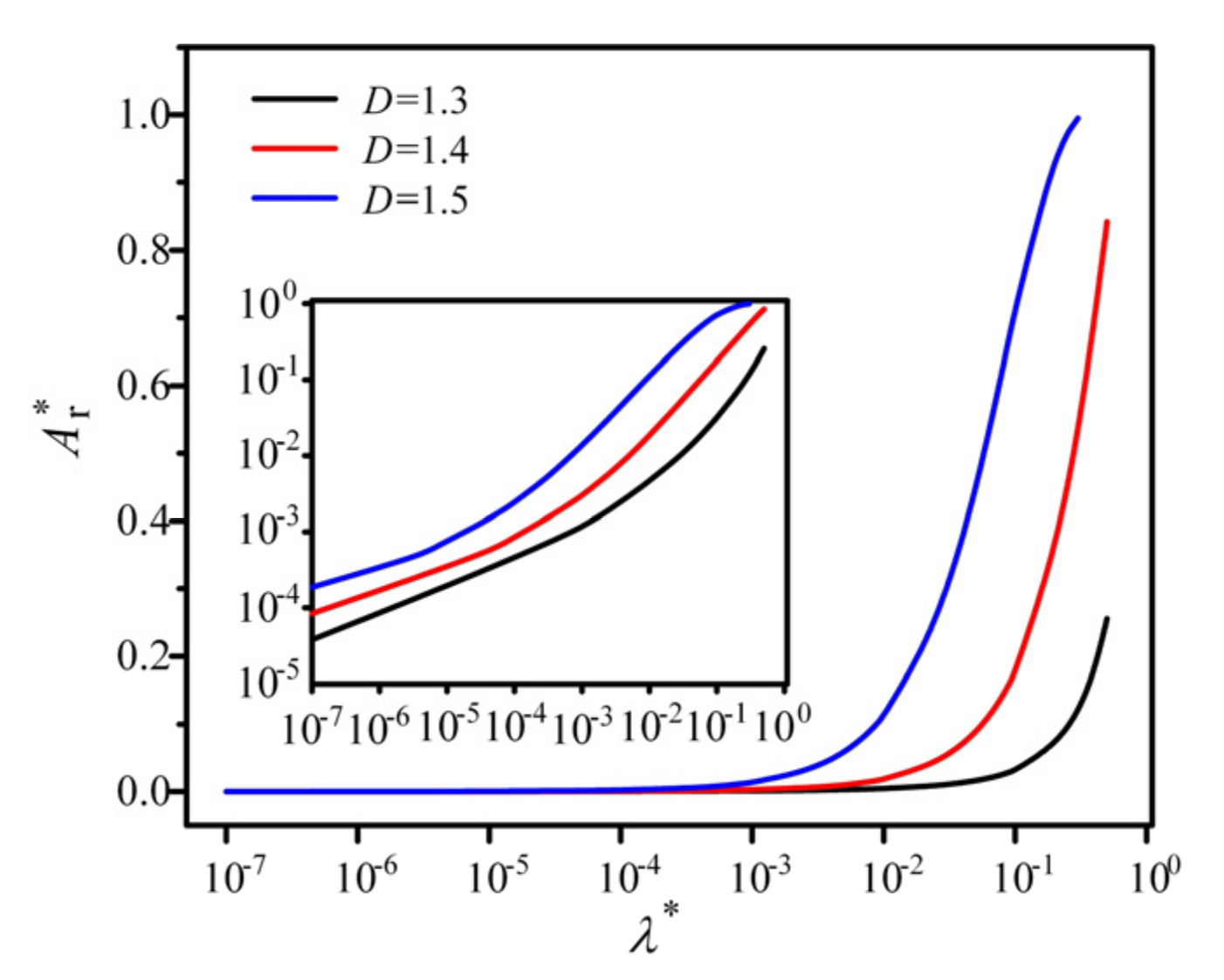
Figure 6 shows that Ar* can be reduced by the decrease in λ* with the same D. Additionally, the observation scale decreases when Ar* begins to reduce with the rising D. It is worth pointing out that Ar* grows as D increases with the same λ*. This is because the surface with a smaller value of D reaches the incomplete contact.
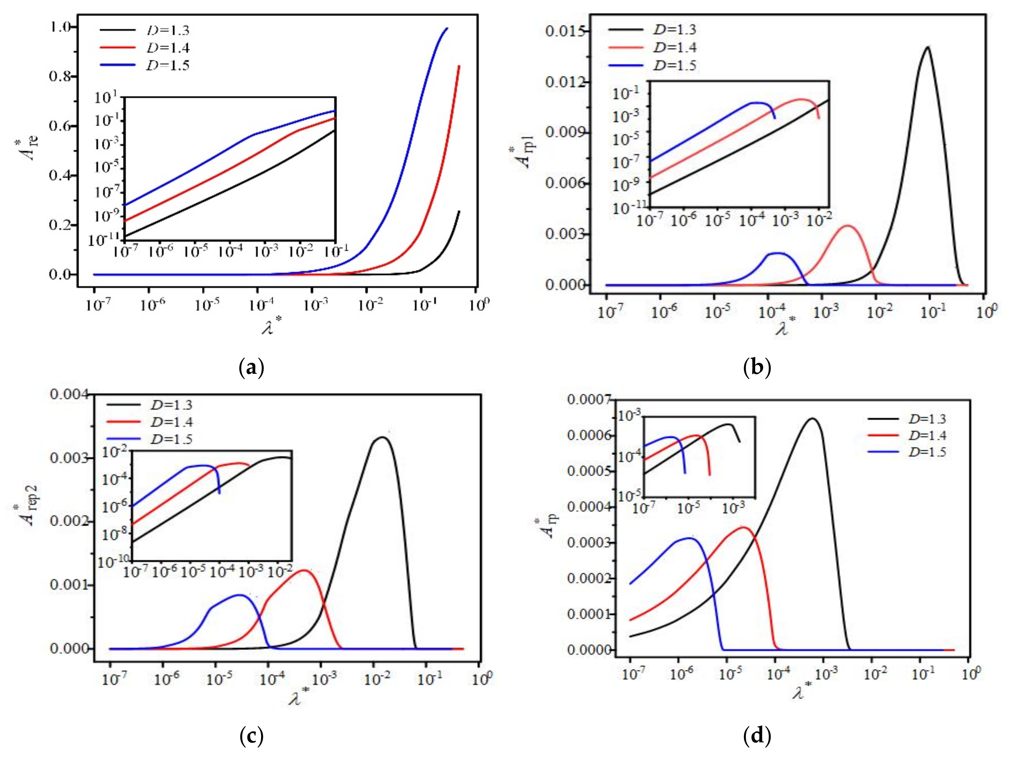
The effects of λ* on the dimensionless contact areas are shown in Figure 7 with G = 1 × 10⁻¹² m and E = 100 GPa. When λ* decreases, the plastic contact dominates, and otherwise, the elastic contact dominates. The dimensionless elastic contact area Are* decreases as λ* reduces, and in the other three stages, the areas rise to the peak before decreasing to a small value. The maximum areas reduce with the increase in D. Moreover, the λ* where peaks occur reduce with the increase in D. For D = 1.3, when the peak occurs, λ* = 0.1, and Arep1* = 0.0142, λ* = 0.02 and Arep2* = 0.0034. For D = 1.4, when the peak occurs, λ* = 0.003, and Arep1* = 0.0036, λ* = 5 × 10⁻⁴ and Arep2* = 0.0012, respectively. In general, the value of D has a large effect on the real contact area Ar* and the area of each deformation stage.
In the elastic deformation stage, when λ* > 0.5, the proportion of Are* is 1, and there is only elastic deformation, as shown in Figure 8. The proportion gradually decreases when (a) D = 1.3 and λ* < 0.4; (b) D = 1.4 and λ* < 0.02; (c) D = 1.5 and λ* < 0.0006. This is because the elastic deformation transforms into the first elastoplastic deformation with the decrease in λ*. For the elastoplastic deformation stage, the trend is similar to that of their dimensionless areas, and the value of the peaks increases as D increases. For the plastic deformation stage, the proportion of the plastic dimensionless area is 0 when (a) D = 1.3 and λ* > 0.002; (b) D = 1.4 and λ* > 9 × 10⁻⁵; (c) D = 1.5 and λ* > 7 × 10⁻⁶. Additionally, when λ* is small enough, there is only plastic deformation.
From the above discussion, it can be seen that there is only elastic deformation at a large λ*. However, with the decrease in λ*, the first elastoplastic and the second elastoplastic contact states become the main contact states successively. Therefore, it is more consistent with reality to consider elastic–plastic deformation.

3.1.2. The Influence of the Equivalent Modulus

In order to study the effects of the equivalent modulus of elasticity, it is assumed that D = 1.3, G = 1 × 10⁻¹² m, ν = 0.3. Figure 9 is the dimensionless real contact area versus λ* with various E:E = 50 GPa, E = 75 GPa, E = 100 GPa.
As shown in Figure 9, the dimensionless real contact areas decrease with λ*. When λ* < 0.2, the areas with various E are nearly the same. Additionally, when λ* > 0.2, a high value of E produces a big slope.
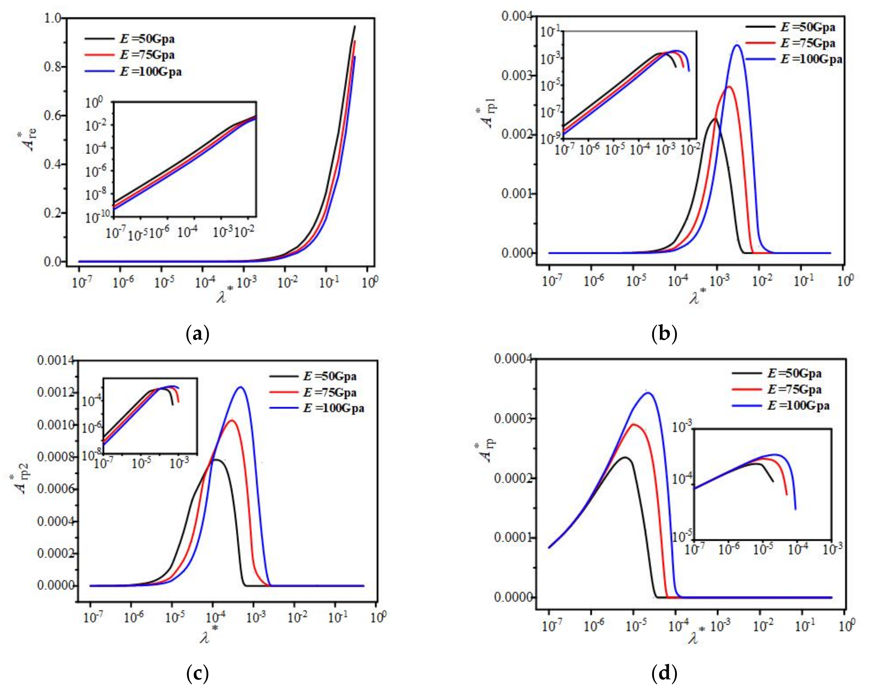
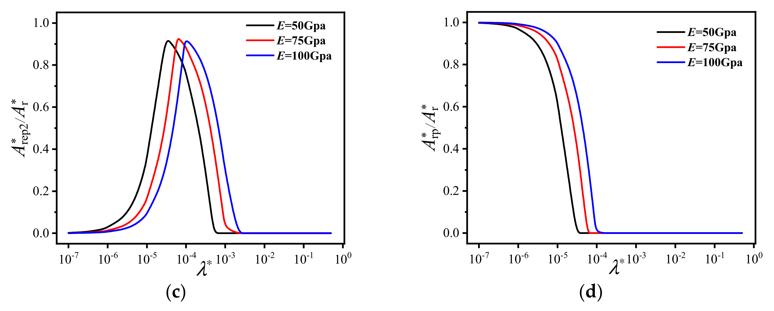
Figure 10 presents the real contact areas in different stages versus λ* with various E. The area Are* decreases with λ*, and a high value of E produces a big slope. As λ* reduces, the areas Arep1*, Arep2* and Arp* rise to the peak before decreasing to a small value. Additionally, the maximum λ* where the area begins to reduce is different with different E. For example, when the area Arep2* begins to reduce, E = 50 GPa and λ* = 7 × 10⁻⁵, E = 75 GPa and λ* = 2 × 10⁻⁴, E = 100 GPa and λ* = 1 × 10⁻⁴.
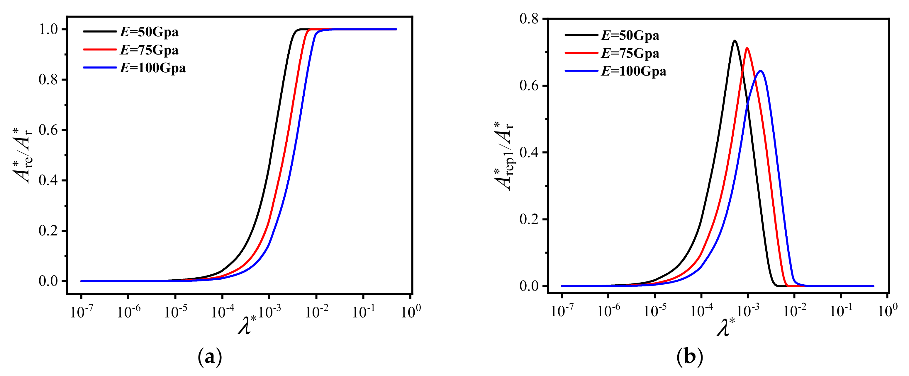
Figure 11 shows the influence of the equivalent modulus of elasticity on multilength contact characteristics. The area Are* decreases with λ*, and a high value of E produces a big slope. Similarly, as λ* reduces, the proportion of Arep* rises to the peak before decreasing to a small value, and the maximum λ*, where the peaks exist, becomes bigger when the value of E becomes higher. As E increases, the peak becomes lower in the first stage of elastoplastic contact, but it remains approximately unchanged in the other stage. The proportion of plastic contact area reduces as λ* increases, and when λ* > 0.001, the proportion is greater than 0.999.

3.2. Model Comparison

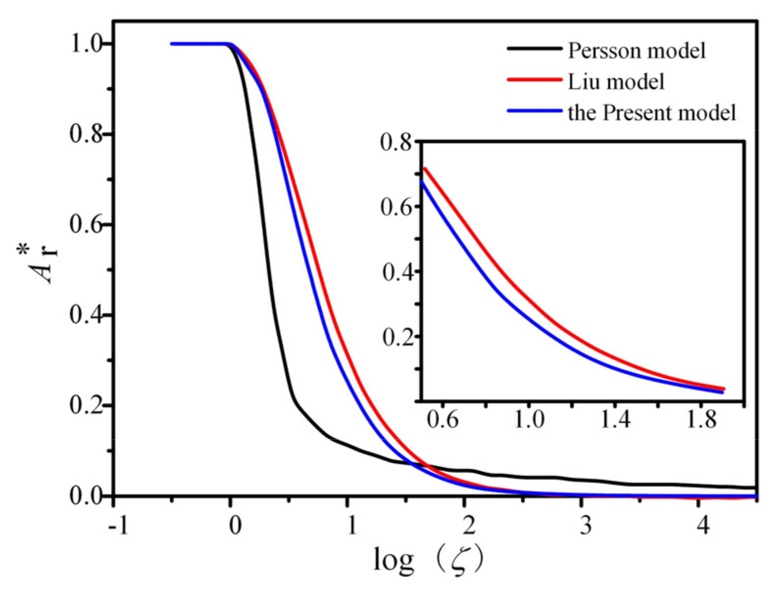
The model is compared to the Liu model and the Persson model to verify its validity. During Persson’s experiment, Persson chose steel and plexiglass as the materials for the contact surface, with the root mean square of rough surface RMS = 0.1 μm, D = 1.2, E = 100 GPa, σY = 1 GPa, and ν. The equivalent parameters of our model are the surface fractal dimensions of 2D surface profile D = 1.2, the sample length L0 = 0.01 m, the fractal roughness parameter G = 1.917 × 10⁻²⁷, the mean contact stress σ0 = 110 MPa. The relationship between the observation scale and the contact area can be obtained according to the multi-scale contact model, as shown in Figure 12. In order to compare with the Persson model, the magnification is defined [26]. The magnification ζ is defined as ζ = λ0/λ where λ0 is the critical value of observation length. When ζ = λ0/λ, the two contact surfaces are in full contact, and Ar* = 1. When ζ = λ0/λ, the two contact surfaces are in full contact, and Ar* = 1. When λ0 < λ, the contact is incomplete, and Ar* < 1.
The dimensionless real contact area Ar* decreases with the rise of ζ and increases with the reduction in λ. The three curves have an inflection point where the real contact area decreases with the observation length. According to the changing rules, the curves can be clearly divided into two parts. They have good consistency in the changing rule and trend. Therefore, the present model is consistent with Liu’s model and Persson’s model.
The present model and the Persson model both have an inflection point at which the real contact area decreases with the observation scale. The pattern of change can be clearly divided into two phases. There is good agreement in the pattern of change and the trend of change. Thus, the validity of the model can be verified. The contact area of the present model is larger compared to the Persson model at a larger observation length (100.25 < ζ < 101.5). This is because the present model replaces the contact areas of the asperities with the ideal subplane areas and obtains a relatively large result. The contact area of the present model is smaller compared to the Persson model at a smaller observation length (ζ > 101.5). This is because Persson assumed that when the local contact is in a plastic state, the plastic contact area will no longer change as the observation length decreases. However, in the present model, after the contact enters into a plastic state, the local surface is still in an incomplete contact. It was suggested that the minimum observation length of the incomplete contact can reach the atomic level.
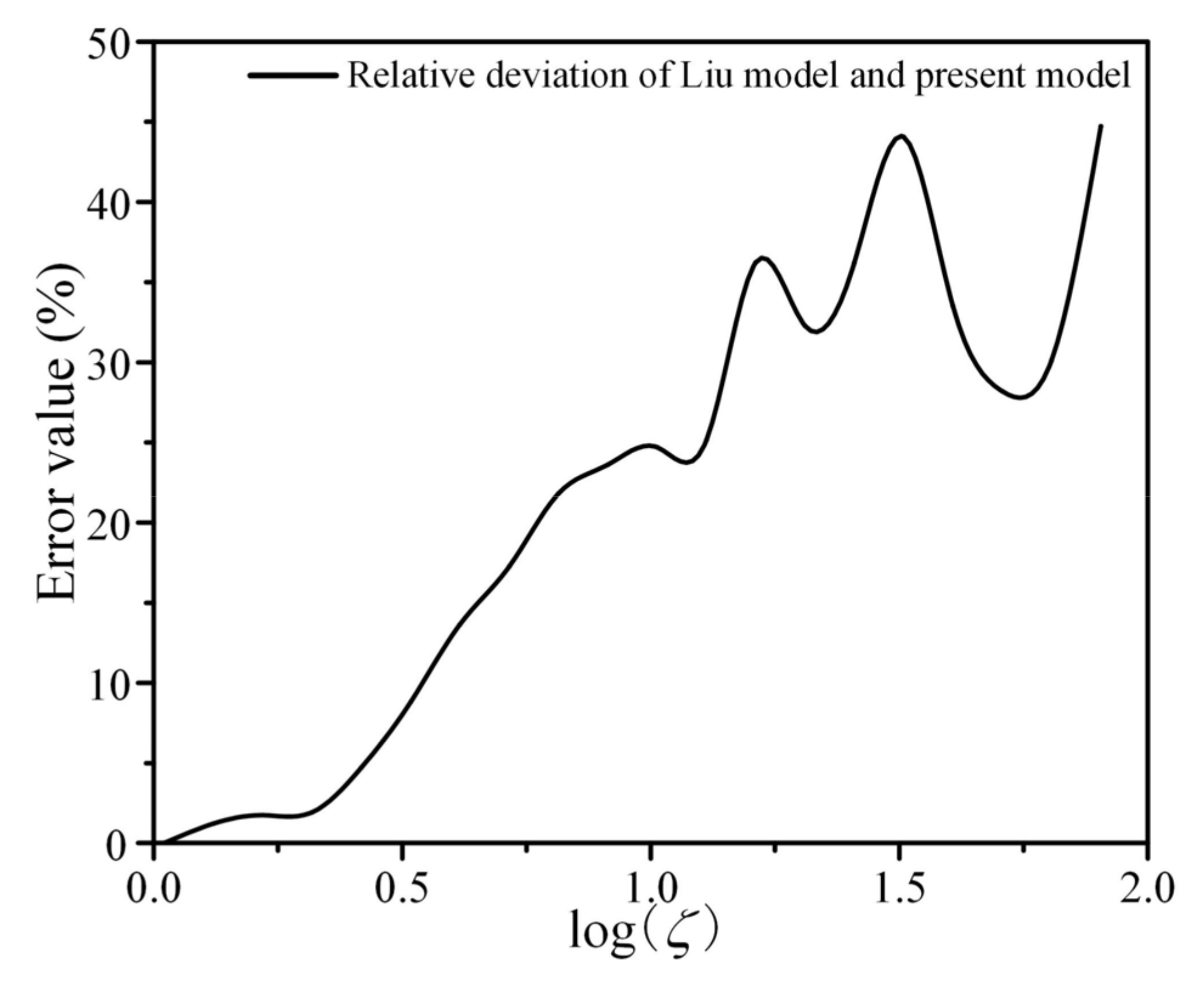
To compare the present model more specifically with the Liu model, Figure 13 is obtained. It shows the error ratio between the Liu model and the present model. It can be seen that the error fluctuates within 0~44.8%. For example, when log ζ = 1.5, the error ratio is 44.6. It can be seen that whether to ignore the elastic–plastic deformation has a large impact on the contact area, especially when the observation length is small.
Therefore, the present model is more accurate than the Persson model, and it is meaningful.

4. Conclusions

In this work, a revised continuous observation length model of rough contact without adhesion based on the statistics method is proposed. The W-M function is used to simulate the rough surface and establish the ideal subplanes. The relationship between the standard deviation and the observation length at different fractal dimensions is fitted in different methods. Moreover, the transition from elastic deformation to plastic deformation is also considered. The mathematical models of forces and areas in different states are proposed, and the change of the areas with λ* are discussed. Additionally, the present model is compared to the Persson model and the Liu model to verify this model. The detailed conclusions are as follows:
  • When the fractal dimension D is different, the fitting relationship between the standard deviation and observation length is also different. For D ≤ 1.5, the polynomial fitting is the best. For D = 1.6, the quadratic polynomial fitting is more in line. For D ≥ 1.7, the ExpDec2 function fitting is better than the other fitting methods. The larger the D, the larger the error of the linear fitting.
  • As λ* reduces, the areas Ar* and Are* decrease, and in the other three stages, the areas rise to the peaks before decreasing to a small value. The values of the peaks and the values of λ* where peaks occur are related to D and E. As λ* reduces, the proportion of Are* decreases, the proportion of Arep* rises to the peak before similarly decreasing to a small value, and the proportion of Arp* increases. When λ* reduces to a certain value, the proportion of Arp* approaches 1, and the proportion of Arep1* is larger than Arep2*.
  • As D increases, the area Ar* increases. The values of the peaks and λ* where peaks occur reduce with rising D. As E increases, the area Are* drops quicker when λ* decreases. Additionally, the values of the peaks and λ* where peaks occur decrease with the increase in E.
  • The dimensionless real contact area of the present model is in good agreement with the Persson model and the Liu model in terms of variation patterns.
  • The present model can accurately describe the contact characteristics of rough surfaces and the monotonicity and continuity in contact processes. The research results provide a theoretical basis for analyzing the contact characteristics on rough surfaces and designing a contact surface topography.

5. The Future Work

In the next stage, the contact force and the contact area of the sealing device of engineering equipment will be studied. To ensure the accuracy of the data, multiple specimens will be used for contact performance testing. Firstly, the surface morphology of the experimental sample of the sealing device is measured to obtain the 2D contour profile. The fractal parameters of the contact surface are calculated, such as the fractal dimension D and the fractal roughness G. Secondly, the experimental setup will be set up, and normal loading experiments will be carried out to obtain the results of contact force, contact depth and contact area. Then, the present theoretical model, material parameters and fractal parameters will be input into Python for programing the calculation. Numerical results are obtained for the contact force and contact area as the contact depth increases. Finally, the experimental results are compared with the theoretical numerical results to verify the rationality of the present model. After modifying the model according to the experimental results, the model can be directly used to calculate the contact force without any experiment, which will save time and costs considerably.

Author Contributions

Conceptualization, L.Z. and J.W.; methodology, M.L. and J.W.; software, J.W. and M.L.; validation, J.W. and G.X.; formal analysis, J.W.; investigation, J.W.; resources, L.Z.; data curation, J.W. and G.X.; writing—original draft preparation, J.W.; writing—review and editing, M.L.; visualization, L.Z.; supervision, L.Z.; project administration, L.Z. All authors have read and agreed to the published version of the manuscript.

Funding

This research received no external funding.

Data Availability Statement

The study did not report any data.

Conflicts of Interest

The authors declare no conflict of interest.

Nomenclature

The notations that were frequently used throughout the article are listed.
λthe observation length, m
λ*the observation scale
λ0the critical value of observation length
xthe height of the ideal subplane
σthe standard deviation
σ (λ)the standard deviation of the ideal subplane
h(λ)the height of the ideal subplane
h(λ)the average height of the ideal subplane
d(λ)the separation at the observation length λ, m
R2the coefficient of determination
z(x)the height of the surface profile
L0the sample length, m
nlthe minimum frequency index
γnspatial frequency
Dthe surface fractal dimension
Gthe fractal roughness, m
Kthe hardness coefficient
νthe Poisson ratio
Hthe hardness of the softer material, MPa
σYthe yield strength, MPa
Rthe asperity curvature radius, m
E1, E2Young’s modulus of two contacting surfaces
ν1, ν2Poisson’s ratios of two contacting surfaces
Ethe equivalent modulus of Hertzian elasticity
Arthe real area of contact surface, m2
Arethe elastic contact area, m2
Arep1the real area in the first stage of elastoplastic contact, m2
Arep2the real area in the second stage of elastoplastic contact, m2
Arpthe real plastic contact area, m2
A0the nominal area, m2
Athe elastic dimensionless contact area
Arep1*the dimensionless area in the first stage of elastoplastic contact
Arep2*the dimensionless area in the second stage of elastoplastic contact
Arp*the plastic dimensionless contact area
Ar*the total dimensionless contact area
Fecthe critical contact force, N
Frethe contact force of single asperity in elastic contact, N
Frep1the contact force of single asperity in the first stage of elastoplastic contact, N
Frep2the contact force of single asperity in the second stage of elastoplastic contact, N
Frpthe contact force of single asperity in plastic contact, N
Prthe total surface contact force
Prethe plastic contact forces, N
Prep1*the dimensionless force in the first stage of elastoplastic contact
Prep2*the dimensionless force in the second stage of elastoplastic contact
Prp*the plastic dimensionless contact force
Pr*the total dimensionless contact force
σ0the mean contact stress, MPa
RMSthe root mean square of rough surface
ζthe magnification

References

  1. Bowden, F.P.; Tabor, D. The Hardness of Metals; Clarendon Press: Oxford, UK, 1951; pp. 279–281. [Google Scholar]
  2. Greenwood, J.A.; Williamson, J.P. Contact of nominally flat surfaces. Proc. R. Soc. Lond. Ser. A Math. Phys. Sci. 1966, 295, 300–319. [Google Scholar] [CrossRef]
  3. Chang, W.; Etsion, I.; Bogy, D.B. An Elastic-Plastic Model for the Contact of Rough Surfaces. J. Tribol. 1987, 109, 257–263. [Google Scholar] [CrossRef]
  4. Xu, Y.; Jackson, R.L.; Marghitu, D.B. Statistical model of nearly complete elastic rough surface contact. Int. J. Solids Struct. 2014, 51, 1075–1088. [Google Scholar] [CrossRef] [Green Version]
  5. Bhushan, B.; Majumdar, A. Role of Fractal Geometry in Roughness Characterization and Contact Mechanics of Surface. J. Tribol. 1990, 112, 205–216. [Google Scholar] [CrossRef]
  6. Zhao, Y.; Maietta, D.M.; Chang, L. An Asperity Microcontact Model Incorporating the Transition from Elastic Deformation to Fully Plastic Flow. J. Tribol. 2000, 122, 86–93. [Google Scholar] [CrossRef]
  7. Liou, J.L.; Lin, J.F. A modified fractal microcontact model developed for asperity heights with variable morphology parameters. Wear 2010, 268, 133–144. [Google Scholar] [CrossRef]
  8. Kogut, L.; Etsion, I. Elastic-plastic contact analysis of a sphere and a rigid flat. J. Appl. Mech. Trans. ASME 2002, 69, 657–662. [Google Scholar] [CrossRef] [Green Version]
  9. Morag, Y.; Etsion, I. Resolving the contradiction of asperities plastic to elastic mode transition in current contact models of fractal rough surfaces. Wear 2007, 262, 624–629. [Google Scholar] [CrossRef]
  10. Yuan, Y.; Gan, L.; Liu, K.; Yang, X. Elastoplastic contact mechanics model of rough surface based on fractal theory. Chin. J. Mech. Eng. 2017, 30, 207–215. [Google Scholar] [CrossRef]
  11. Hanaor, D.A.H.; Gan, Y.X.; Einav, I. Contact mechanics of fractal surfaces by spline assisted discretisation. Int. J. Solids Struct. 2015, 59, 121–131. [Google Scholar] [CrossRef]
  12. Pan, W.; Song, C.; Ling, L.; Qu, H.; Wang, M. Unloading contact mechanics analysis of elastic–plastic fractal surface. Arch. Appl. Mech. 2021, 91, 2697–2712. [Google Scholar] [CrossRef]
  13. Wen, Y.; Tang, J.; Zhou, W.; Li, L.; Zhu, C. New analytical model of elastic-plastic contact for three-dimensional rough surfaces considering interaction of asperities. Friction 2021, 10, 217–231. [Google Scholar] [CrossRef]
  14. Zhang, W.; Jin, F.; Zhang, S.L.; Guo, X. Adhesive Contact on Randomly Rough Surfaces Based on the Double-Hertz Model. J. Appl. Mech. Trans. ASME 2014, 81, 051008. [Google Scholar] [CrossRef]
  15. Song, H.; Van der Giessen, E.; Liu, X. Strain gradient plasticity analysis of elasto-plastic contact between rough surfaces. J. Mech. Phys. Solids 2016, 96, 18–28. [Google Scholar] [CrossRef] [Green Version]
  16. Song, H.; Vakis, A.I.; Liu, X.; Van der Giessen, E. Statistical model of rough surface contact accounting for size-dependent plasticity and asperity interaction. J. Mech. Phys. Solids 2017, 106, 1–14. [Google Scholar] [CrossRef] [Green Version]
  17. Kuzkin, V.A.; Kachanov, M. Contact of rough surfaces: Conductance-stiffness connection for contacting transversely isotropic half-spaces. Int. J. Eng. Sci. 2015, 97, 1–5. [Google Scholar] [CrossRef]
  18. Jin, F.; Wan, Q.; Guo, X. Plane Contact and Partial Slip Behaviors of Elastic Layers With Randomly Rough Surfaces. J. Appl. Mech. Trans. ASME 2015, 82, 091006. [Google Scholar] [CrossRef]
  19. Chen, Q.; Xu, F.; Liu, P.; Fan, H. Research on fractal model of normal contact stiffness between two spheroidal joint surfaces considering friction factor. Tribol. Int. 2016, 97, 253–264. [Google Scholar] [CrossRef]
  20. Pan, W.; Li, X.; Wang, L.; Guo, N.; Mu, J. A normal contact stiffness fractal prediction model of dry-friction rough surface and experimental verification. Eur. J. Mech. A Solids 2017, 66, 94–102. [Google Scholar] [CrossRef]
  21. Wang, R.; Zhu, L.; Zhu, C. Research on fractal model of normal contact stiffness for mechanical joint considering asperity interaction. Int. J. Mech. Sci. 2017, 134, 357–369. [Google Scholar] [CrossRef]
  22. Zhai, C.; Hanaor, D.; Gan, Y. Contact stiffness of multiscale surfaces by truncation analysis. Int. J. Mech. Sci. 2017, 131, 305–316. [Google Scholar] [CrossRef]
  23. Yuan, Y.; Chen, J.J.; Zhang, L.H. Loading-unloading contact model between three-dimensional fractal rough surfaces. AIP Adv. 2018, 8, 075017. [Google Scholar] [CrossRef] [Green Version]
  24. Wang, H.H.; Jia, P.; Wang, L.Q.; Yun, F.H.; Wang, G.; Liu, M.; Wang, X.Y. Modeling of the Loading-Unloading Contact of Two Cylindrical Rough Surfaces with Friction. Appl. Sci. 2020, 10, 742. [Google Scholar] [CrossRef] [Green Version]
  25. Persson, B.N.J. Contact Mechanics for Randomly Rough Surfaces. Surf. Sci. Rep. 2006, 61, 201–227. [Google Scholar] [CrossRef] [Green Version]
  26. Afferrante, L.; Bottiglione, F.; Putignano, C.; Persson, B.N.J.; Carbone, G. Elastic Contact Mechanics of Randomly Rough Surfaces: An Assessment of Advanced Asperity Models and Persson’s Theory. Tribol. Lett. 2018, 66, 75. [Google Scholar] [CrossRef]
  27. Ciavarella, M. An approximate JKR solution for a general contact, including rough contacts. J. Mech. Phys. Solids 2018, 114, 209–218. [Google Scholar] [CrossRef] [Green Version]
  28. Guo, X.; Ma, B.B.; Zhu, Y.C. A magnification-based multi-asperity (MBMA) model of rough contact without adhesion. J. Mech. Phys. Solids 2019, 133, 103724. [Google Scholar] [CrossRef]
  29. Liu, M.; Zhang, L.; Wang, L.Q.; Liu, H.X.; Sun, Y.Q.; Wang, Y.J. The leakage analysis of submarine pipeline connecter based on a new fractal porous media model. Desalin. Water Treat. 2020, 188, 390–399. [Google Scholar] [CrossRef]
  30. Lorenz, B.; Persson, B.N.J. Leak rate of seals: Effective-medium theory and comparison with experiment. Eur. Phys. J. E 2010, 31, 159–167. [Google Scholar] [CrossRef] [Green Version]
  31. Persson, B.N.J. Leakage of Metallic Seals: Role of Plastic Deformations. Tribol. Lett. 2016, 63, 42. [Google Scholar] [CrossRef]
  32. Lorenz, B.; Rodriguez, N.; Mangiagalli, P.; Persson, B.N.J. Role of hydrophobicity on interfacial fluid flow: Theory and some applications. Eur. Phys. J. E 2014, 37, 57. [Google Scholar] [CrossRef] [PubMed]
  33. Rodriguez, N.; Dorogin, L.; Chew, K.T.; Persson, B.N.J. Adhesion, friction and viscoelastic properties for non-aged and aged Styrene Butadiene rubber. Tribol. Int. 2018, 121, 78–83. [Google Scholar] [CrossRef]
  34. Persson, B.N.J.; Scaraggi, M. Theory of adhesion: Role of surface roughness. J. Chem. Phys. 2014, 141, 124701. [Google Scholar] [CrossRef] [PubMed] [Green Version]
  35. Persson, B.N.J. The dependency of adhesion and friction on electrostatic attraction. J. Chem. Phys. 2018, 148, 144701. [Google Scholar] [CrossRef] [PubMed]
  36. Tiwari, A.; Dorogin, L.; Tahir, M.; Stockelhuber, K.W.; Heinrich, G.; Espallargas, N.; Persson, B.N.J. Rubber contact mechanics: Adhesion, friction and leakage of seals. Soft Matter 2017, 13, 9103–9121. [Google Scholar] [CrossRef] [PubMed]
  37. Persson, B.N.J.; Scaraggi, M. Some Comments on Hydrogel and Cartilage Contact Mechanics and Friction. Tribol. Lett. 2018, 66, 23. [Google Scholar] [CrossRef]
  38. Lorenz, B.; Persson, B.N.J. Leak rate of seals: Comparison of theory with experiment. Europhys. Lett. 2009, 86, 44006. [Google Scholar] [CrossRef]
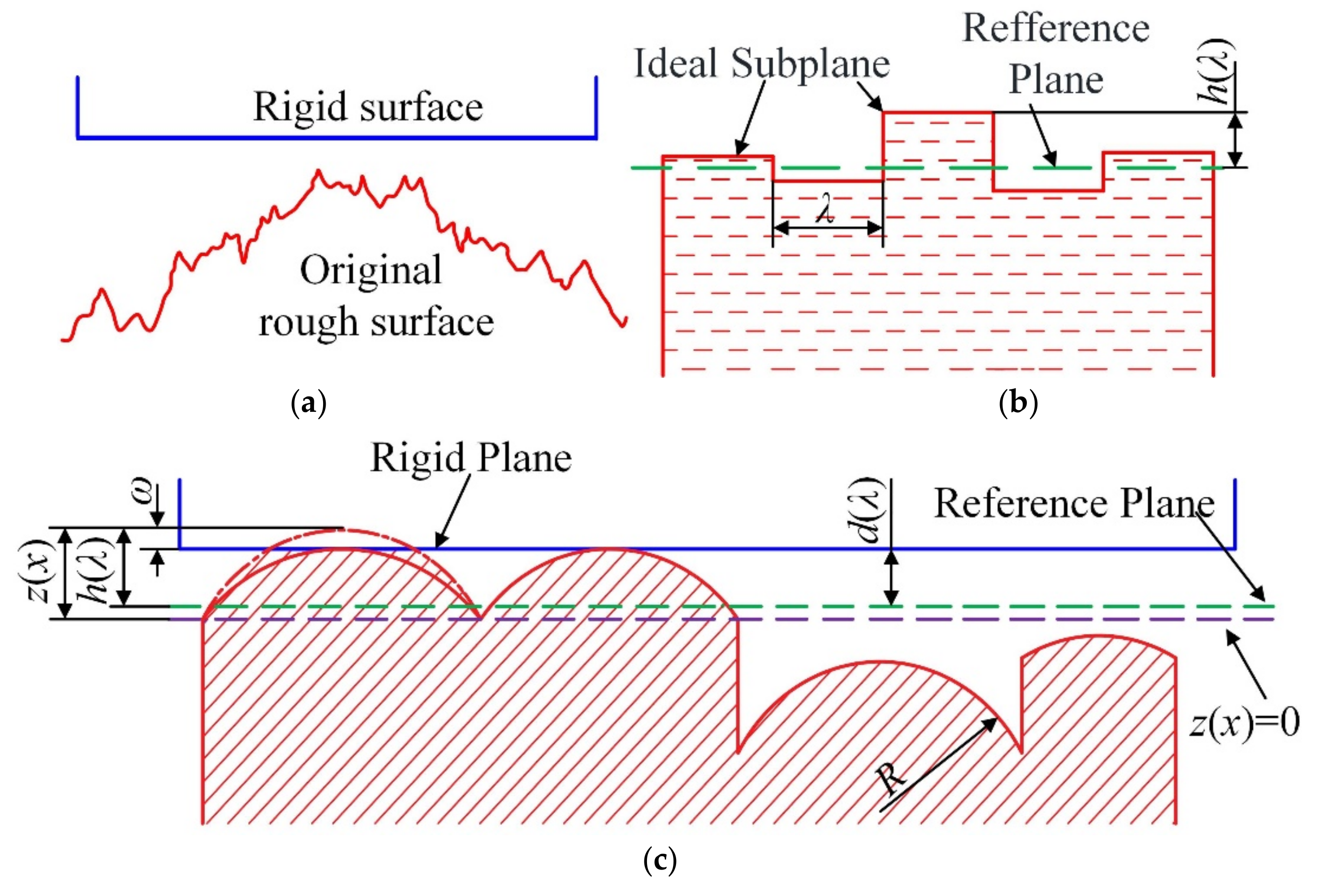
Figure 1. The contact of two rough surfaces. (a) The contact of two rough surfaces can be idealized as a rigid plane pressed on a deformable rough surface. (b) The fractal surface can be regarded as a discrete surface composed of ideal subplanes. (c) The fractal surface can be regarded as asperities of the same curvature radius.
Mathematics 10 03764 g001
Figure 2. The calculated standard deviation σ of the ideal subplane height with various fractal dimensions.
Mathematics 10 03764 g002
Figure 3. The different fitting curves between the dimensionless observation length and the standard deviation at different fractal dimensions (D ≤ 1.5).
Mathematics 10 03764 g003
Figure 4. Different fitting curves between the dimensionless observation length and the standard deviation at different fractal dimensions. (a) Linear fitting, Quadratic fitting and Cubic fitting at D = 1.7. (d) ExpDec2 fitting at D = 1.7, 1.8 and 1.9.
Mathematics 10 03764 g004
Figure 5. The relationship between R2 and D.
Mathematics 10 03764 g005
Figure 6. The real contact area versus observation scale λ* with various D.
Mathematics 10 03764 g006
Figure 7. The real contact area Ar* in different contact stages versus λ* with various D. (a) Dimensionless elastic deformation area Are* versus λ*. (b) Dimensionless elastoplastic deformation area Arep1* in the first stage versus λ*. (c) Dimensionless elastoplastic deformation area Arep2* in the second stage versus λ*. (d) Dimensionless plastic deformation area. Arp* versus λ*.
Mathematics 10 03764 g007
Figure 8. Influence of surface fractal dimension on multilength contact characteristics. (a) Proportion of elastic contact area versus λ*. (b) Proportion of elastoplastic contact area in the first stage versus λ*. (c) Proportion of elastoplastic contact area in the second stage versus λ*. (d) Proportion of plastic contact area versus λ*.
Mathematics 10 03764 g008
Figure 9. Dimensionless real contact area versus observation scale λ* with various E.
Mathematics 10 03764 g009
Figure 10. The real contact area Ar* in different contact stages versus the λ* with various E. (a) Dimensionless elastic contact area Are* versus λ*. (b) Dimensionless elastoplastic contact area Arep1* in the first stage versus λ*. (c) Dimensionless elastoplastic contact area Arep2* in the second stage versus λ*. (d) Dimensionless plastic contact area Arp* versus λ*.
Mathematics 10 03764 g010
Figure 11. Influence of equivalent modulus of elasticity E on multilength contact characteristics. (a) Proportion of elastic contact area versus λ*. (b) Proportion of elastoplastic contact area in the first stage versus λ*. (c) Proportion of elastoplastic contact area in the second stage versus λ*. (d) Proportion of plastic contact area versus λ*.
Mathematics 10 03764 g011aMathematics 10 03764 g011b
Figure 12. Comparison between models.
Mathematics 10 03764 g012
Figure 13. The error ratio between the Liu model and the present model.
Mathematics 10 03764 g013
Table 1. The parameters of surface profiles.
ParametersValues and Units
D1.1~1.9
G10−12 m
L00.01 m
λmin1.0 × 10−9 m
Publisher’s Note: MDPI stays neutral with regard to jurisdictional claims in published maps and institutional affiliations.