Article

A Combined Dynamic Programming and Simulation Approach to the Sizing of the Low-Level Order-Picking Area

Faculty of Transport and Traffic Engineering, University of Belgrade, 11120 Beograd, Serbia
*
Author to whom correspondence should be addressed.
Mathematics 2022, 10(20), 3733; https://doi.org/10.3390/math10203733
Submission received: 16 September 2022 / Revised: 4 October 2022 / Accepted: 7 October 2022 / Published: 11 October 2022

Abstract

:
In order to increase the efficiency of the order-picking process, warehouses are forced to find ways to adopt to constantly intensifying changes in the assortment and quantities of stored products. Accordingly, we present a methodology that deals with such a problem at a tactical level by defining the optimal size and an allocation of products within the order-picking area of the most typical order-picking setting. The methodology combined two methods, dynamic programming and simulation modelling, with the aim of taking advantages of their positive features. In that sense, the optimal allocation of products for different sizes of the order-picking zone were obtained by the dynamic programming approach. Afterwards, the influence of a demand’s seasonality and variations were treated by the simulation model, so that the more realistic performances of the system were captured for the optimal allocation of products. The methodology was tested on the retailer data with significant week seasonality. The obtained results confirmed the practical applicability of the methodology in real systems, while the sensitivity analysis of results showed that special attention and effort should be given to the determination of costs related to the engagement of order-pikers, storage equipment and unit replenishment during a planning period.

1. Introduction

Adaptation to changes is a must and a prerequisite in providing efficient and competitive logistics service. According to [1] “since warehousing does not add value to the final product, the effort is placed on obtaining efficiency in costs, such as minimizing movements, workforce, equipment, and energy consumption, among other cost drivers”. Because of the complex structure and mutual interactions of warehouse processes [2,3], frequently with opposed goals, the optimization of every aspect of warehouse operation is a must for achieving warehouse efficiency. An activity that, according to [4], occupies 50–75% of all operating costs is order-picking. Therefore, any optimization of the order-picking process, referred in the rest of the paper just as order-picking, increases warehouse efficiency.
Order-picking is “the process of retrieving products from storage (or buffer areas) in response to a specific customer request” [5], and it has long been identified as the most labor-intensive and costly activity for almost every warehouse. Performances of the order-picking process, such as throughput, response times, error rate level, costs, etc., highly depend on the applied technological concept. We use the term technological concept to comprise the following elements of an order-picking warehouse system: a technology implemented in an order-picking area (OPA); a spatial form of the OPA; and an organization and control of the order-picking process. Accordingly, an appropriate selection of mentioned technological concept elements has a crucial role in creating the appropriate preconditions for the maximization of performances of the order-picking process. A particularly important aspect is the design of a suitable OPA [6,7].
OPA (sometimes named forward picking area) is a subsystem of the warehouse dedicated to the order-picking activities. In accordance, this area is designed and tailored according to the requirements of the order-picking process with the aim of its efficient realization. Therefore, depending on the goals of the strategic levels of a warehouse, OPA may occupy only one part of a warehouse’s surface, or the whole warehouse. It can include only the lowest rack level(s), or all levels. Eventually, it can be customized in several ways so that it satisfies higher goals. On the other side, the reserve area is a warehouse subsystem designed exclusively for storing bulk pallets, which are used for the replenishment of empty pallets in the OPA. The problem of designing the OPA is a complex problem, characterized by numerous interdependent decisions, such as the selection of an appropriate OPA type; selection of an OPA technology and a method of executing the order-picking process; defining OPA’s size; determination of the quantity of assigned products in the OPA, etc. [5,8,9]. Moreover, all decisions are made in the presence of conflicting objectives and the existence of many potentially applicable solutions.
On one side, the use of the OPA improves the efficiency of order-picking by reducing the traveled distances. However, on the other, it implies an additional replenishment of the products from the reserve area to the OPA, imposing the double handling of goods. Accordingly, it is obvious that a larger OPA generates higher costs related to the necessary storage equipment, occupied warehouse space and overall order-picking distances, while it reduces replenishments costs. Oppositely, smaller OPA requires less storage equipment, occupies less space and induces shorter order-picker routes, but at the same time, it increases the intensities of replenishing flows. Therefore, one of the crucial decisions in designing OPA is to adequately determine the size of the OPA, as well as to define which products should be assigned to the OPA and in what quantity. According to [10], these decisions should balance the costs of order-picking and replenishing processes so that the benefits of the OPA are maximized.
Besides the mentioned cost trade-off, the choice of the technological concept also has a significant impact on the determination of the OPA size. The technological concept’s features define the framework in which the size of the OPA is determined. Namely, the technological concept which implies that order-picking is executed exclusively in the OPA usually has different goals and constraints compared to the technological concept which allows picking from the reserve area. Moreover, certain technological concepts assume that interference between the realization of the order-picking and the OPA’s fulfillment processes are negligible and therefore imply their simultaneous realization. On the other side, other technological concepts assume that such interference has a sufficiently significant impact on flows’ performances within the OPA so that replenishment during the order-picking has to be minimized as much as possible. In the latter cases, this usually means that the content of the OPA (i.e., its size, types and quantities of products) must be determined and provided before the beginning of the order-picking to satisfy expected demand during the planning period in the highest possible rate. In that way, the number of replenishment operations that are executed during the order-picking process will be minimized. This type of technological concept is widely present both in the practice and in the literature [11] and it is the presumption that we used in this research. This means that the additional goal of sizing the OPA is the minimization of emergency replenishments during the realization of order-picking process.
Regarding space characteristics of the technological concept, the most typical technological concept solution for the case picking is the vertical division of the conventional selective pallet rack [5]. The lower level of the pallet rack is assigned to the OPA for order-picking while the upper rack levels represent the reserve area.
This research considers the technological concept characterized by the vertical division of storage space and the realization of the order-picking process exclusively within the low-level OPA. In the considered technological concept, the reserve area is used twofold. On one side, it is used for storing inventories, while on the other it is used for picking bulk pallets for orders in which the quantity of ordered products exceeds one pallet. Therefore, another assumption of the considered problem is that each product on the order-picking list is demanded in a quantity that does not exceed the content of one pallet. Otherwise, the separation of OPA and reserve area is meaningless.
The considered technological concept also implies such a work organization in which the preparation of OPA, regarding the provision of expected quantities of products in the following period, is performed before the picking period only by replenishment of bulk pallets. Pallets whose contents were not used entirely in the previous order-picking process are not re-filled to the full capacity because it requires a significant increase in replenishing process time. Namely, it means that a full pallet must be brought in the OPA on a forklift, one part of it must be transferred to the pallet that is being refilled, and eventually, the brought pallet must be returned to the reserve area. This replenishing process slightly increases the possibility of emergency replenishment during the order-picking process, but it simplifies the OPA preparation for the following period and therefore it is more present in practice. In the case of a possible lack of products in the OPA during the period, emergency replenishment of the products is performed from the reserve area by bulk pallets.
In conformity with the previous, the goal of our research was to provide a methodology for sizing OPA with respect to the described technological concept and availability of required data. Since the considered technological concept is widely implemented in warehouses that are already operating, practical implementation of the given methodology is not related only to the design of new warehouses, but also to the periodic reconfiguration of existing ones.
Accordingly, the main contribution of this research is the development of a new methodology for sizing OPA with stochastic demand during the order-picking process. The implementation of the cost model in methodology simultaneously covers several mutually confronting performances of the order picking zone, and therefore contributes to making more comprehensive solutions. In this way this research fills the gap that exists in the literature which deals with the sizing OPA under the considered technological concept. Moreover, it should be mentioned that the methodology is not limited to the considered technological concept, meaning that it can be universally applied under the condition that specificities of the considered technological concept are considered.
The following parts of the paper are organized as follows. In Section 2, we give a literature review. In Section 3, we formulate the considered problem, which is afterward solved by the procedure given in Section 4. Finally, in Section 5, we present the results of numerical experiments conducted with the goal to test the proposed procedure, and in Section 6 we give some concluding remarks.

2. Literature Review

Research related to various warehouse problems is widely present in the scientific literature. Comprehensive overviews of papers devoted to different classes of warehousing problems are given in [2,3,5,9,12]. However, to emphasize the differences of the considered problem and problems in previous studies, the scope of the literature review is limited to papers that are related to the OPA problems. Moreover, the review is organized into two parts. In the first part, the focus is on the OPA design decision problems treated so far in studies, while in the second part, we give an overview of methods used in studies. The overview of the most significant papers together with implemented solution methods is given in Table 1.

2.1. Design Decision Problems

Hackman et al. [13] developed a heuristic procedure to determine which products to assign to the OPA (AS/RS serves as an OPA) and how to allocate space among the assigned products, given the OPA has fixed capacity. They made heuristic attempts to minimize the total costs for order-picking and replenishment. Frazelle et al. [14] considered a situation where the size of the OPA is a decision variable. The costs they considered included the OPA’s equipment cost and the order-picking material handling cost, as well as cost of the internal replenishment. They used the heuristic method of Hackman et al. [13] as the basis for their solution method.
The problem that considers a unit load replenishment, which means that only one unit of goods can be replenished in a trip, was considered by Van den Berg et al. [11]. The main assumption of their research was that OPA can be replenished momentarily, and therefore there is no reason to store more than one unit of a product in the OPA. Additionally, they assumed that the warehouse operation implies the existence of busy and idle working periods and showed that by performing the majority of replenishments during the preceding idle periods it is possible to reduce the number of emergency replenishments during the following busy period. A set of products to be placed within the OPA, with the objective to minimize an expected work of resources in order-picking and emergency replenishing activities during the busy period, is achieved by implementing a knapsac-based algorithm. In [15], Bartholdi and Hackman dealt with less than one case storage unit, which is a usual quantity for warehouses that store small parts. The results of the two storing strategies, typically used in practice, were compared with the optimal strategy used for small parts.
Gu et al. [10] proposed an alternative branch-and-bound based algorithm that quickly solves, to the optimality, the forward-reserve allocation problem. Computational results demonstrated that the branch-and-bound algorithm was fast enough to solve problems of practical sizes. Moreover, the applicability of greedy heuristics by Hackman et al. [13] to real, practical problems showed that the solutions were close to optimal with a negligible difference.
All previous research has mainly focused on a simplified version of the problem (usually denoted as fluid models), which implies that the OPA can be subdivided continuously. Walter et al. [22] investigated the discrete version of the OPA in which the authors analyzed the model gaps between the fluid models and their discrete alternatives.
Thomas and Meller [23] presented a methodology, based on statistical analysis, to develop guidelines useful to design a manual case-picking warehouse. The guidelines aimed at minimizing the total labor by providing an initial warehouse design and by considering all relevant warehouse characteristics. Their methodology was limited to defining the size and the layout of the OPA, configuration of the loading docks and a shape and height of a pallet rack. In [21], the authors determined the size of the OPA with the objective of achieving a desired service level while simultaneously respecting the dynamism and variability of the demand levels. The considered problem was set up for the warehouse of the cosmetic products in which a separate order-picking area was installed for the service of on-line orders. The solution of the problem was obtained from the utilization of the analytical model. However, although it tackled the problem of the OPA sizing, this type of problem also differs from the problem considered in this research due to the different type of the OPA.

2.2. Applied Solution Methods

In general, in the literature devoted to solving various warehouse order-picking problems, analytical, mathematical programming and simulation models are used in the majority of cases. Detailed overviews of the application of these methods, for solving the combinations of tactical and operational problems in the case of the man-to-goods systems, have been given in the available literature [12].
From all mentioned methods, the simulation is traditionally the most widely applied method, for example Van Gils et al. [12] stated it was used in cca. 51% of reviewed papers. Generally, simulation is mostly used for the validation of warehouse project decisions. Moreover, most of the operational research models were validated by simulation [24]. In the following paragraphs we give a brief overview of some of the research that has utilized simulation as a modelling tool.
Baker and Canessa [8] recommended the utilization of simulation in the following steps of the framework: establishing the unit load; selection of equipment; calculating the capacity; and performance evaluation. Altarazi et al. [25] proposed an approach for the design of manual-order-picking warehouses based on simulation modelling. The proposed approach extended the search space for performance improvement by investigating all possible warehousing design combinations with their stochastic nature and interactions. Bahrami et al. [16] used the simulation analysis as a tool for assessing a contribution of the new OPA allocation strategy on the order picking process performances. Numerous studies have demonstrated the applicability of simulations in several warehousing design elements. Caron et al. [26] presented a simulation approach for an efficient manual order-picking warehouse layout design that uses either random or cube per order index storage policies. By using simulations, Petersen [27] considered the effect of the warehouse configuration on the total travelled time. The warehouse configuration was represented by the number of aisles per zone and the length of aisles. In order to analyze the influence of several picking, routing, and storage policies on the total distance required to satisfy picking tasks, Petersen and Aase [28] utilized a simulation model. They also performed a sensitivity analysis of the effect of order size, warehouse shape and demand distribution. Roodbergen and Vis [29] developed an approach for defining the optimal layout of one block of parallel aisles OPA with the objective of minimizing average route lengths of order-pickers. Average length of order-pickers’ routes was calculated according to an analytical formula based on two (the S-shaped and the largest-gap) the most widely used order-picker routing heuristic policies. Suitability of the given analytical formula was confirmed by the utilization of the simulation model. Later Roodbergen et al. [30] presented a model for defining an optimal layout structure of OPA with an arbitrary number of blocks with parallel aisles. In this case, the authors gave a statistical assessment of the average length of an order-picking route for the case of random assignment of pallet locations over the warehouse and implementation of the S-shape routing policy of order-picker. Validation of the statistical assessment was also confirmed by a simulation experiment. Roodbergen et al. [31] presented a simulation-based warehouse design method while concurrently considering scenarios of layout and operational policies. Simulation was utilized to determine the performance of the various resulting scenarios. The results revealed a large potential for improving warehouse performances. Winkelhaus et al. [32] investigated the possibility of implementing a hybrid order-picking system, made as a combination of an autonomous robot and a human order-picker in the OPA. Authors used a simulation model to analyze the performances of such a system for different characteristics of order-picking tasks. Jiang et al. [24] considered a robotized warehouse in which robots bring order-picking shelves to the OPA. The focus of the paper was on the operational control of the replenishing process of the OPA, as well as on the order-picking process. Synchronization of these two processes was modeled by a heuristic model based on the VNS metaheuristics. The effectiveness of the solutions obtained by the VNS was compared to the conventional method of synchronizations whose performance parameters are gathered by a simulation model. Lolli et al. [33] considered a warehouse of finished goods and an order-picking system based on the goods-to-man setting in which they faced problems of dimensioning: the size of the OPA, a number of order-pickers and a number of automated guided vehicles. Authors used a quing theory-based model for the simultaneous dimensioning of all required parameters, and a simulation model for the purpose of validation.
In papers [17,18,19] devoted to OPA, the dominant solving approach was the application of heuristic models which allow a complex observed problem to be solved with accepted accuracy and calculation time. However, in the case of the considered problem, due to the tactical problem nature, the time does not play a critical role which is a reason why we did not propose a heuristic algorithm. Moreover, as it will be seen from numerical results, time required for solving real life problem sizes can be considered as more than acceptable.
The analysis of reference papers [11,13,14,15,20,22,23] devoted to the solution of OPA indicated that developed models are not suitable for direct application in the case of the type of technological concept considered in this research. For example, Frazelle et al. [14] treated the technological concept that allows case-picking from the reserve area, which is not acceptable for the considered technological concept. The assumption of the continuity of OPA’s space and capacity represented in [13,14,15] is the basic constraint for implementation of their solutions within the considered technological concept, due to discrete capacities of OPA expressed in a number of pallet locations (more details in Walter et al. [22]). Moreover, the assumption from [23] that different products in OPA are represented only with one pallet is not acceptable in the considered technological concept because the number of pallets with products is a decision variable. In [20], the authors analyzed the benefits of the implementation of the OPA within an automated storage/retrieval system (AS/RS) which is a representative of goods-to-man order-picking concept. They compared the performances of the ABC allocation strategy of products within the AS/RS with the strategy of making separate OPA within the AS/RS. According to the results obtained by the analytical model, they made a recommendation in which situations, i.e., under which circumstances it is justified to for an OPA within an AS/RS. However, this research also dealt with different types of OPA settings.
Finally, it should be emphasized that, as even two decades ago the authors stressed in [9], the need for design-oriented studies is still present, especially at the tactical level of design because of the longer influence of such decisions on warehouses’ operations and the efficiency. In that sense, as it can be seen in Table 1, this paper fills the gap in the literature by simultaneous considering two crucial OPA sizing problems: dimensioning of the OPA and the allocation of products within the OPA for a given set of products to be assigned to the OPA and for the specific settings of the order-picking process. Bearing in mind the availability of relevant data at this stage of warehouse design, to the best of our knowledge, there are no studies that have treated such a problem with the implemented technological concept.

3. Problem Formulation

In this section, we summarize the information about the considered technological concept given in Section 1 and complement the technological concept’s settings necessary to completely define the conditions in which OPA sizing procedure is implemented. Accordingly, the procedure was developed under the following assumptions:
  • Layouts of OPA and reserve area are already defined;
  • All requests for order-picking in the picking period are realized in the OPA;
  • Assortment of products in the OPA is already known, based on the expected demand in a planning period;
  • At least one pallet of every product is present in the OPA;
  • Before the picking period, there is sufficient time to provide the necessary quantity of products to the OPA;
  • In the event of a lack of certain product in the OPA, emergency replenishments are performed during the picking period;
  • The quantity of products in one emergency replenishments cycle is equal to one pallet of products;
  • Demand of each product i (i = 1, …, N) during the picking period (expressed in case units) is described by Normal distribution Ni ~ (μi, σi), where μi is expected demand for the product i, and σi is standard deviation of the demand of the same product during the picking period. It should be noted that the normal distribution is the result of summing all individual product’s demands during the order-picking period, i.e., all demands of orders. As it is well known, regardless of distributions of added variables, an aggregated variable tends to follow the normal distribution even for a small number of added variables;
  • Number of case units per pallet is npi (i = 1, …, N).

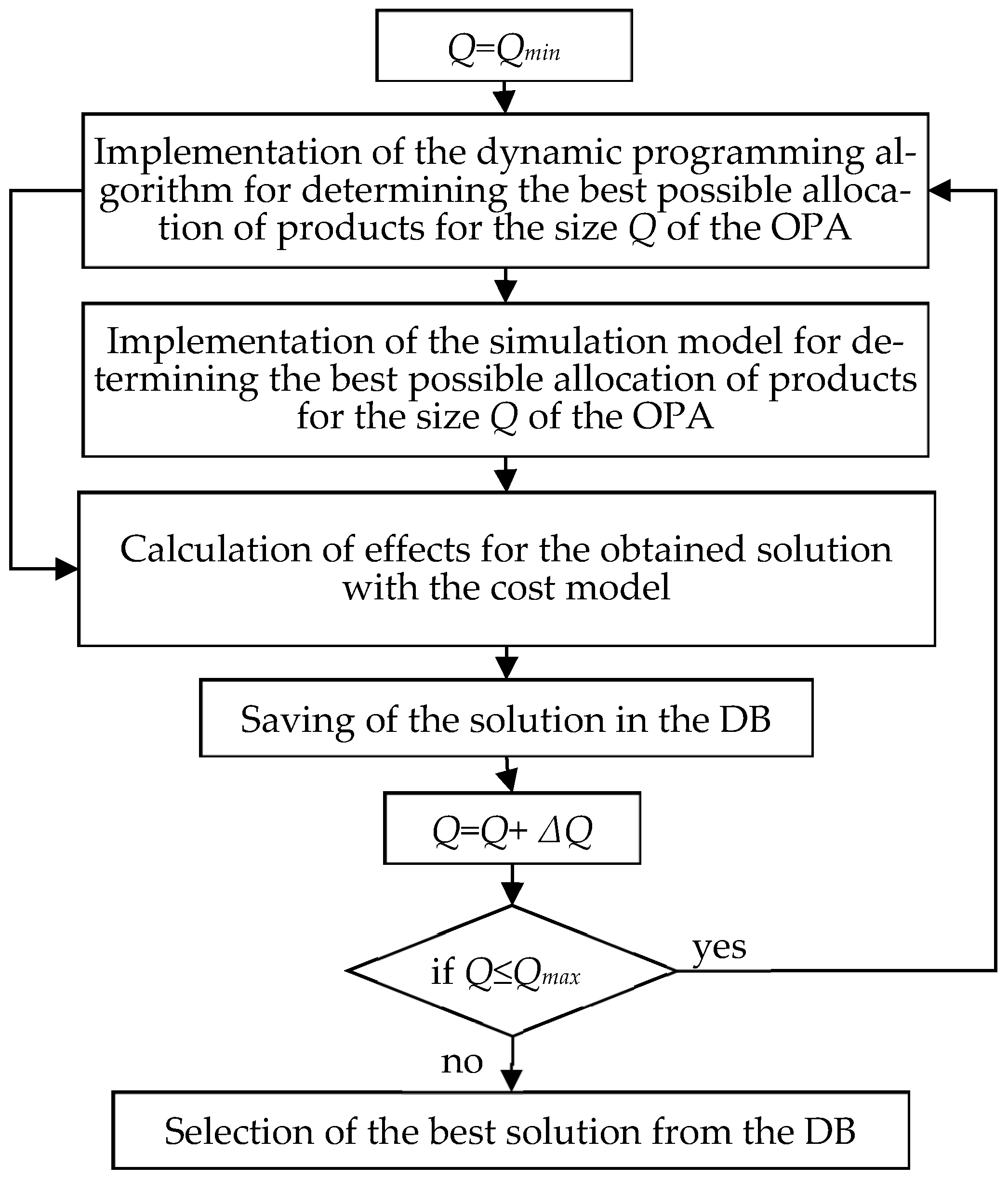
4. Solution Procedure

The proposed procedure implies the implementation of the iterative approach in defining the optimal OPA size. In each step of such procedure the appropriate effects for a particular size of the OPA (Q) are determined by using the cost model. Effects related to the OPA size are stored in the database (DB). The initial size of the OPA is Qmin, while in every iteration the OPA size is increased by ΔQ. The procedure ends when OPA size exceeds the maximum size Qmax, i.e., the number of steps of the procedure is ( Q max Q min ) / Δ Q . Eventually, the analysis of the results from the DB determines the most favorable OPA size. An overview of the procedure is given in Figure 1.
According to the conditions and limitations of the technological concept, Qmin is usually equal to the number of products that are picked up during the selected picking period, i.e., Qmin = N. The maximum number of pallet locations Qmax corresponds either to the total demand for products in the picking period (expressed in pallet units) or to the maximal number of pallets that could be stored in the OPA. The step of changing the capacity ΔQ (expressed in the number of pallets) is adapted to the technical and technological characteristics of the warehouse equipment and the space for OPA in the technological concept.
In the development of a contemporary OPA, besides the costs of its formation and operation, service level becomes one of the most important criteria. Here it should be noted that by the service level we consider a complex feature of a system that indicates the quality of the service that the system provides to its users (it usually includes response time, accuracy, probability of request realization, etc.). Within the service level, the minimization of the time needed for order realization is often set as the goal. Observed in the context of the technological concept, the maximization of the service level is achieved if the OPA enables the order processing during the picking period to be realized with the minimum number of emergency replenishments from the reserve area. In this way, besides the efficiency of order-picking, the safety in the OPA is also increased.
Based on the defined criteria, the effect of considered capacity (Q) is determined by solving the allocation–assignment (AA) problem. It is necessary to emphasize that for the analyzed technological concept, AA is reduced only to the problem of allocation because all products are picked exclusively from the OPA, and hence they must be present in the OPA.
To solve this problem, we applied the optimization model based on the dynamic programming. The main goal of the AA problem is to determine the best possible allocation of the considered OPA size (Q) to products, in terms of minimizing the number of emergency replenishments during the order-picking period. The corresponding effects are evaluated using the cost model. Descriptions of the implemented optimization and cost models are given in the following two sections.

4.1. Optimization Model of Allocation

In the available literature, numerous approaches have been used to solve the proposed allocation problem, such as enumeration (in cases of the problems of smaller dimensions), Lagrange multiplier [34], dynamic programming [17,35] and different heuristic procedures [10,13,14,17].
Notations used in the model formulation are as follows:
  • N—the number of products in the OPA;
  • T—order-picking period (shift, day, week, etc.);
  • Di—a random variable that represents the demand for the product i (i = 1, …, N) expressed in the number of pallet units in T;
  • mi—the maximum expected demand (in pallet units) for the product i during T;
  • Ri—a variable that represents a number of replenishments of the product i during T;
  • Zi—the number of pallet units of the product i assigned to the OPA at the beginning of T;
  • Q—total OPA capacity (expressed in the number of pallet locations);
  • qi—the number of pallets in the OPA assigned to the product i, i = 1, …, N; qi = 1, …, mi;
  • P(qi)—the probability of satisfying the demand for the product i from the OPA during T from the qi pallets of that product;
  • P ( q i ) = P ( D i q i n p i ) = P ( z q i n p i μ i σ i ) = Φ ( z ) + 0.5 . The satisfaction rate is derived from the value of the standard Laplace function Φ ( z ) = 1 2 π 0 z e μ 2 2 d μ . Analogously, P(0) = 0, and for every q i m i P(qi) = 1;
  • P—the probability of satisfying the demand from the OPA during T. P = i = 1 N P i ;
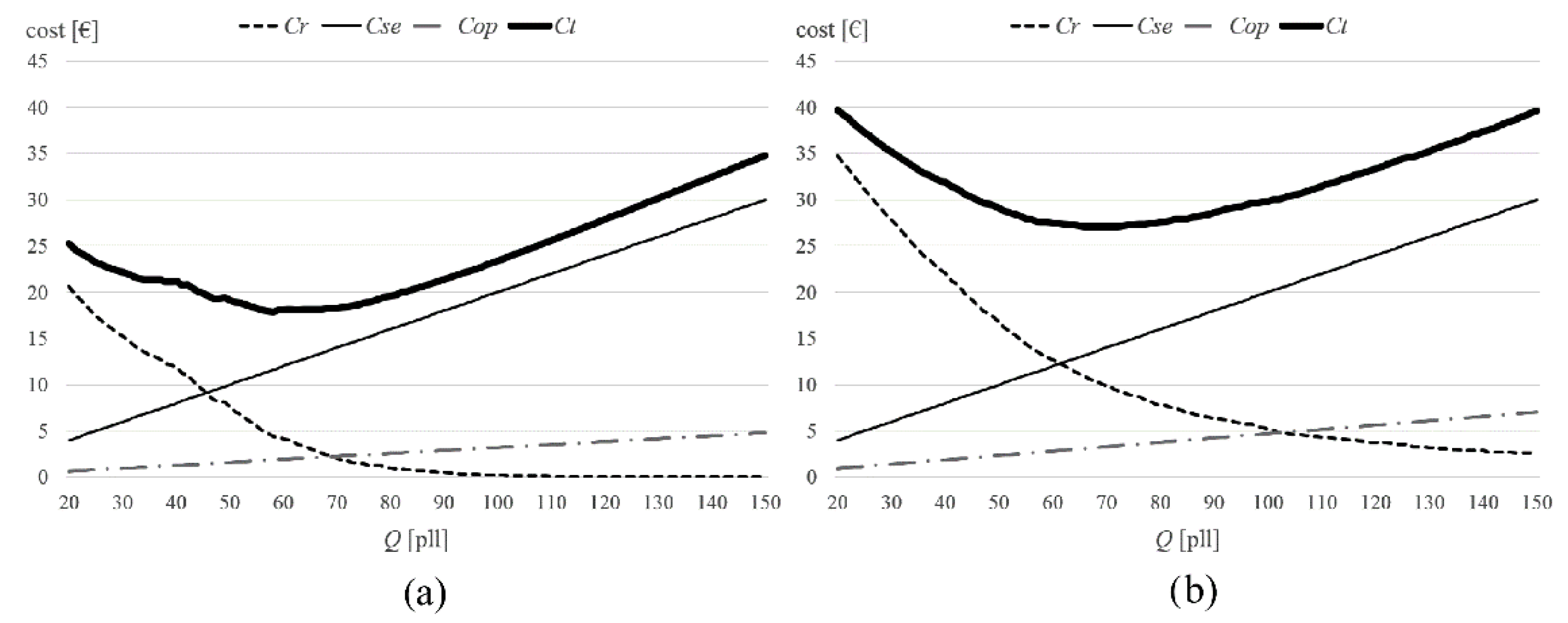
  • Cop (Q)—specific order-picking costs;
  • nd—total number of orders in the observed period;
  • lOPA—length of the order-picking path; corresponds to the number of pallet locations (OPA capacity) in OPA expressed in kilometers;
  • vop—the average speed of an order-picker in OPA (km/h);
  • top—hourly salary of one order-picker during T (EUR/h);
  • Cr (Q)—replenishments costs of the OPA in the observed period of time;
  • tr—the price of one replenishment (€/replenishment);
  • Cse (Q)—specific costs of space and equipment in the OPA;
  • tse—unit price per pallet location (space + equipment) (EUR/pallet location) for the observed period;
  • S—number of remaining unallocated pallet places;
  • qi*—optimal number of products allocated to the OPA;
  • E_repl—the number of emergency replenishments of considered product in a simulation model;
  • N_repl—the number of regular replenishments of considered product in a simulation model;
  • Tmax—the length of a simulation run (in days);
  • Sim_replications—the number of simulations run replications for a given solution.
The required number of emergency replenishments for the OPA during the picking period is dependent on the probability with which the allocated quantities of products meet the demand during that period. In line with this position, it is possible to pose this problem as a problem of space allocation (allocation of remaining pallet locations in the OPA of the product) so that the P is maximized. Therefore, the optimization model of the allocation has the following form:
max P = i = 1 N P ( q i )
so that:
i = 1 N q i = Q
1 q i m i i 1 , ,   N
However, because of the nonlinear nature of the objective function, we implemented a dynamic programming approach for finding the optimal solution of the problem. Accordingly, the maximum value of P for given Q is determined by implementing the following recursive function:
f i ( S ) = max 1 q i min ( m i , S ) { P ( q i ) f i + 1 ( S q i ) }
The search for the optimal solution is of an iterative nature, meaning that for each product and all remaining number of unallocated pallet places (S) every possible number of qi (i.e., for 1 q i m i ) is evaluated. Eventually, the combination of qi that provides the maximum value of P is selected as the optimal number of products (qi*) allocated to the OPA. It should be mentioned that due to the iterative nature of the algorithm, S denotes the number of available pallet locations in OPA for allocation of the ith, i+1th, …. Nth product, combined. Moreover, the value of S at the beginning of the algorithm is equal to the Q. The computational complexity of such dynamic programming algorithm is O ( S 2 N ) .
Based on the obtained qi*, it is possible to determine the total expected number of emergency replenishments during the picking period for all products as i = 1 N R i , where Ri has been calculated as:
R i = k = q i * + 1 m i ( k q i * ) P ( k )
Finally, by applying the dynamic programming algorithm to the selected capacity values within the interval (Qmin ÷ Qmax), a set of optimal allocation values and the probability of the OPA service is obtained. For the final decision of the OPA size, it is necessary to include in the analysis the cost of forming and operating in the OPA. The implemented cost model is given in the following section.

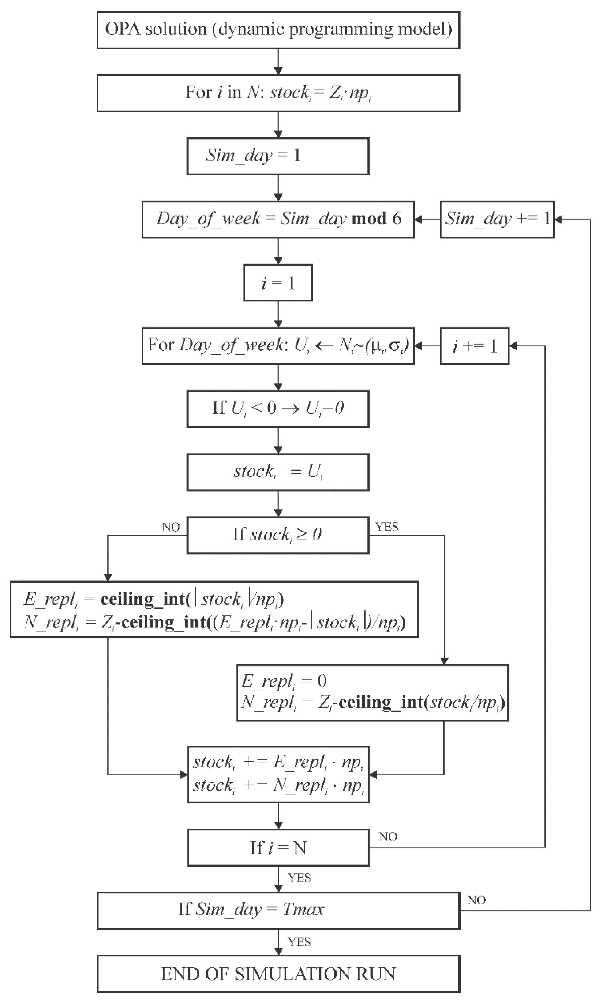
4.2. Simulation Model

The dynamic programming approach described in the previous part gives an optimal solution for stochastic demand values which are represented by the normal distribution. A single continuous order-picking period can be observed as one period in a working day. Therefore, the demand’s mean and standard deviation per product can be obtained as daily values in some past period (e.g., in one quarter of a year). In general, each working day of a week has different demand intensities (values of demand mean and standard deviation). For example, some products can have an increase in demand on Fridays, due to the coming weekend and high consumption from customers (which incurs a somewhat higher rate of emergency replenishments), or a decrease in demand on Mondays (which incurs a somewhat lower rate of emergency replenishments). In that context, a mean of average daily demand could lead to a solution with an intolerable rate of emergency replenishments for some days of a week. On the other hand, if a higher representative of a mean of an average demand is used, total costs can be significantly increased due to the increase in the OPA size and related Cop and Cse costs. Therefore, different calculation methods to obtain the representative mean and standard deviation of a daily demand per product can have a different impact on the total costs of OPA and should be analyzed by the simulation approach.
The second reason for implementing a simulation analysis lies in the fact that the dynamic programming model presumes 100% full stock of products in OPA at the start of each order-picking period (day). This assumption would require case unit replenishment of OPA from the reserve area which is not acceptable in most real-life systems (OPA is replenished with bulk pallets only due to the high intensity of operations required in the case unit replenishment). A total of 100% full stock of products in OPA at the start of the order-picking period is common only at the go-live of OPA setup. For the rest of the days, products usually have partial pallet leftovers from the previous order-picking day.
To test the quality of solutions obtained from the dynamic programming approach, we developed the simulation model presented in the algorithm and the pseudocode forms given in Figure 2 and Algorithm 1, respectively. For the OPA size Q and representative demand’s mean and standard deviation, we applied the dynamic programming model. We set the size and allocation of products in the OPA according to that optimal solution. Based on the actual working day demand mean and standard deviation (Table 2), we randomly generated daily consumption for each product (starting from Monday). Based on the starting stock and the demand, we calculated the stock at the end of that day for all products. If the stock of a product has a negative value, then emergency replenishments (R = E_repl) are required. The number of emergency replenishments depends on that negative value, as presented in Figure 2 and Algorithm 1. After the order-picking time (end of order-picking period), regular replenishments (N_repl) are made to fill the OPA for the next order-picking day. If the stock of a product has a positive value, only regular replenishments are made. Both replenishment types are completed with full pallets (which is a common practice) up to the maximal allocated space represented in the number of allocated pallets. The length of the simulation run (Tmax) spanned several weeks. Each dynamic programming solution was tested with multiple simulation run replications (Sim_replications).
Algorithm 1: Pseudo-code of the simulation model.
for OPA_sol in DP_solutions:  # OPA_sol represents a variant of representative demand data
     for sim_iter in Sim_replications:
       for Sim_day in range (1, Tmax):  #where Sim_day =1 is Monday
         define Day_of_week for Sim_day #what is the day in a week
         for i in range (1, N): #for all products
            for Day_of_week: UiNi~(μi, δi) # generate demand Ui for product i
            stocki = stockiUi
            if stocki <= 0: # if stocki has negative value
               E_repli ← ceiling_int(abs(stocki))  # emergency replenishment (full pallets)
               stocki = stocki + E_repli
            if stocki < Zi: # if stocki is lower than planned value Zi in OPA
              N_repli ← ceiling_int(Zi - stocki) # regular replenishment (full pallets)
               stocki = stocki + N_repli

4.3. Cost Model

The cost model enables the estimation of the cost of order-picking and replenishment processes and the cost of forming the OPA (space and equipment costs). For the purposes of dimensioning, it needs to be presented in the function of the OPA size.
The cost of order-picking (Cop) in the OPA is possible to be determined with the assumption that the order-picker passes all the locations in the OPA when fulfilling the order. This is the usual operating mode for OPA in warehouses due to the large number of lines on a typical order list.
In addition, for the estimation of the Cop, it is necessary to have the data related to the speed of movement and the cost of work of the order-picker. Eventually, the calculation of order-picking costs (in EUR/period) is given by:
C o p ( Q i j ) = n d l O P A v o p t o p
Replenishments’ cost (Cr) can be determined as a function of the required number of replenishments (expression (5)) and the price of one replenishment (EUR/replenishment).
C r ( Q ) = i = 1 N R i t r
In case of emergency replenishments, additional costs may arise due to obstruction/slowdown of the order-picker’s work.
Space and equipment cost (Cse) are directly proportional to the number of pallet locations (OPA size) and the unit price (space and equipment) per pallet location.
C s e ( Q ) = Q t s e
The expression for total costs (in EUR/period) is summed up by these partial costs (6–8):
C t ( Q ) = C o p ( Q ) + C r ( Q ) + C s e ( Q )
The obtained results are stored in the appropriate database (DB). To obtain the optimum, the results from the DB are analyzed, and an optimal OPA size solution is obtained based on the minimum function of the total cost.

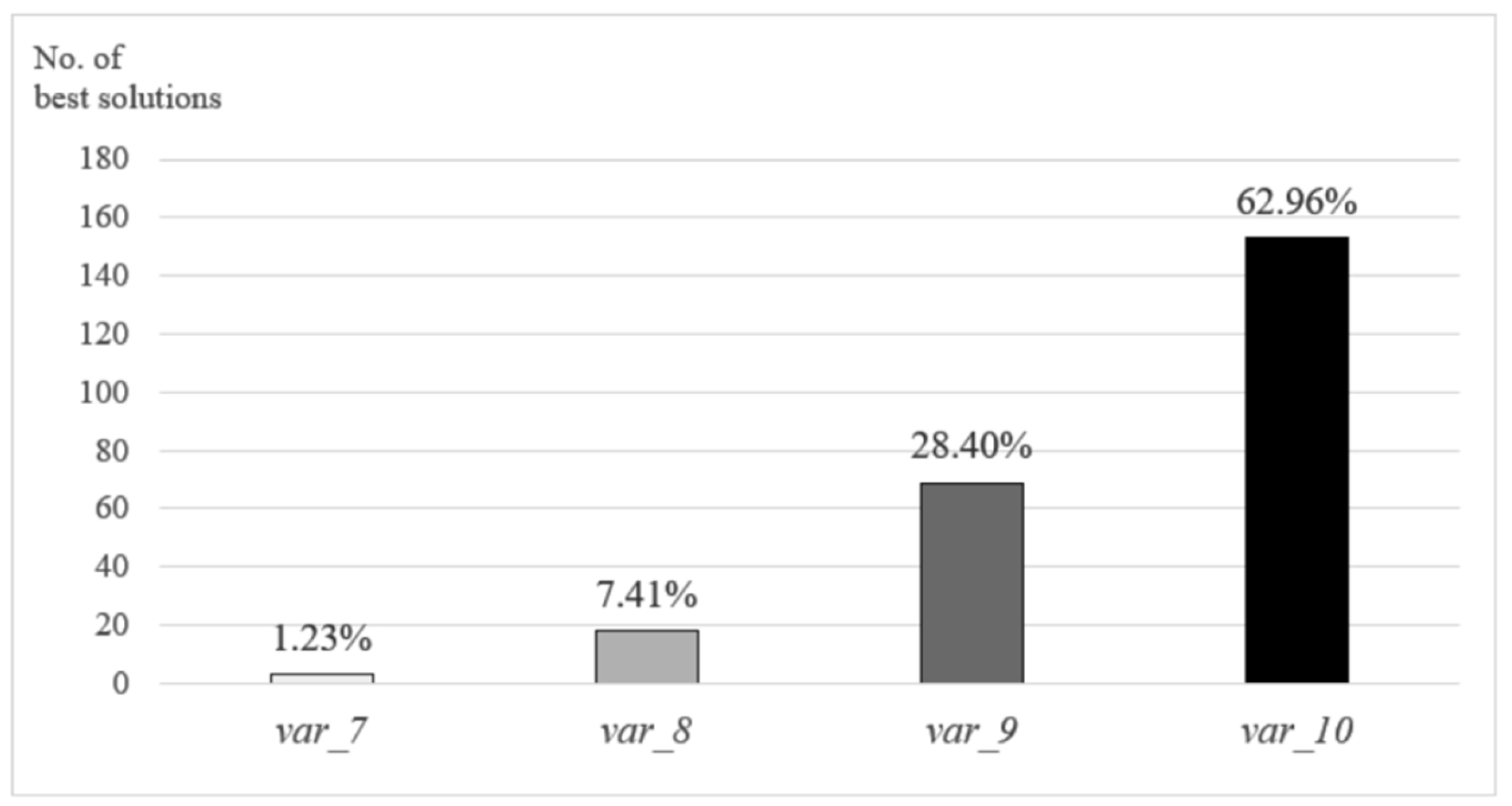
5. Case Study Computational Results

To test our integrated dynamic programming and simulation approach to solving OPA size and allocation, we used case study data from the main distribution center of a worldwide retail chain located in Serbia that supplies over 400 retail stores of different sizes. The data were obtained for the observation period July–September 2018 where over 10,000 different products were shipped from the distribution center. We selected 20 products whose average daily demand exceeded one pallet which were adequate candidates to be served from the OPA, according to the considered technological concept. The reason for their goodness as candidates for the OPA is that on some days of a week, demand is larger than one pallet and more than one pallet is needed to be placed in the OPA. All other products are also present in the OPA but are stored in quantities less than one pallet and with the possibility of storing multiple products in a single storage location, depending on their storing quantities and required space. It should be noted that order-picking of products in the OPA stored in less than one pallet was not the subject of this research due to usually different implemented order-picking technological concept. The order-picking is made in a single working shift, six days a week. Table 2 contains case study data regarding the observed products: number of case units per pallet (npi), the demand’s mean and standard deviations in case units per each working day, as well as the mean and standard deviations in case units calculated as daily values (regardless of the day of a week) for the entire observation period.
The basic variant with average daily demand (var_0 from Table 2), as well as additional variants of demand of representative products calculations (presented in Table 3), were used to obtain the solution by dynamic programming model. These variants were:
  • var_0—daily demand mean and standard deviation calculated from the entire sample of 12 weeks;
  • var_1, var_3, var_5, var_7, var_9, var_11—demand’s mean and standard deviation are equal to a day with 1st, 2nd, 3rd, 4th, 5th and 6th highest mean value, respectively (including average daily demand in the set of days);
  • var_2, var_4, var_6, var_8, var_10, var_12—demand’s mean and standard deviation are equal to a day with 1st, 2nd, 3rd, 4th, 5th and 6th highest value of μi+3σi, respectively (including average daily demand in the set of days).
Each variant has a unique structure of demand parameters for products, where variants with odd numeration give more significance to the mean demand, while variants with even numeration give more significance to standard deviation of a demand.
Values of other input parameters were:
  • The average driving speed of order-picker Vop (1.5 km/h);
  • The cost of the order-picker (2 EUR/h);
  • The width of the pallet location (1 m);
  • Storage price (prices were based on the research and analysis of the prices of services provided by local providers with correction (reduction) for a profit rate of 15–20%) per week (0.2 EUR/pal per day);
  • Price per emergency replenishment (1 EUR/pal).
The dynamic programming and simulation models were implemented using the Python 3.6 programming language on PC Intel(R) Core (TM) i5-3470 CPU @3.20GHz with 8 GB RAM memory.
The best results obtained from the proposed models for different variants of representative demands are presented in Table 4. As expected, the dynamic programming model gave a lower total cost for less intensive representative demands: variants var_11 and var_12 with an average demand of 72.59 and 69.48 case units per product, respectively. The dynamic programming model took into consideration only the representative demand values for obtaining the OPA size solution, while the simulation model took those solutions and tested them in an environment with real demands per each working day. Based on the 12-week length of each simulation run (Tmax = 12 ∗ 6) and 500 replications (Sim_replications), the simulation returned the lowest average total costs ( C t ¯ = 27.08) for the dynamic programming solution with var_10 and OPA size Q = 67 pallets.
Detailed results for the best variant of the representative demand calculation (var_10) from the two models, as well as the allocation of products, are presented in Table 5. Graphical presentation of solution costs for var_10 and different values of Q are given in Figure 3. In general, the simulation model “followed” the costs curve from the dynamic model but with slightly higher values due to the more realistic simulation environment in two aspects: there cannot be a negative demand (in the cases when random generator returns negative demand, that demand is set to zero); and products usually have partial pallet leftovers from the previous order-picking day (100% full stock of products in OPA is certain only on the start of simulation run). The CPU time to obtain dynamic programming solution was relatively low (under 3 s for Q = 150 and N = 20) and allowed its application to OPA size problems of larger dimensions. The CPU time for 500 replications was under 4 s.

5.1. Sensitivity Analysis of the Proposed Approach

For the purpose of sensitivity analysis of the dynamic programming and simulation approach, we generated two additional sets of data regarding main input parameter values: set I with low variations; set II with high variations. The main input parameters observed in the sensitivity analysis were demand mean and standard deviation (μii), as well as unit price intensities (tr, tse, top). The input variation intensities per two sets were:
  • For set I, all parameters could take 90%, 100% or 110% of their original values from the case study;
  • For set II, all parameters could take 50%, 100% or 200% of their original values from the case study.
Because of a large number of instances to be solved by different variants of representative demand calculation (in total both sets had 243 combinations of parameters), we reduced the analysis complexity by increasing Q from 20 by step 4 (10, 28, 32, etc.). This simplification did not have a significant influence on the sensitivity analysis.

5.1.1. Computational Results for Set I—Low Variations

The dynamic programming and simulation models solved instances for Q from 20 to 150 (the largest Q size of best solution from dynamic programming model was 140 for instance with [μi, σi, tr, tse, top] = [1.1, 1.1, 1.1, 0.9, 0.9]).
Regarding the percentage (out of total 243 combinations) of the best solution found after the simulation approach, var_10 showed the best results with 62.96% (Figure 4), followed by var_9, var_8 and var_7, respectively. Other variants were not able to obtain a solution with the lowest total cost. The results showed that the proposed approach was not significantly sensitive to small changes in input parameters’ values, especially because var_9 and var_10 had similar values of representative demand parameters (with average demand at 83.13 and 82.61, respectively) and they jointly obtained the best results in 91.36% of cases.
According to Table 6, the proposed approach was most sensitive to the costs of emergency replenishment (tr) and order-picker (top). The graphical representation of the required Q in solutions with the lowest total costs per each combination of input parameters is given in Figure 5. The OPA size Q took values between 56 and 88 pallets, where 85% of the best solutions had Q between 60 and 78 pallets.

5.1.2. Computational Results for Set II—High Variations

The dynamic programming and simulation models solved instances for Q from 20 to 250 (the largest Q size of the best solution from the dynamic programming model was 220 for instance with [μi, σi, tr, tse, top] = [2, 2, 2, 0.5, 0.5]). We excluded var1–4 from the analysis because they did not provide good quality solutions, and we left var0, 5–6 and 11–12 in the analysis because they were close (by average demand intensity) to the four variants that provided at least some of the best results for set I.
The significantly higher variation intensity of the main input parameters led to “allocation of quality” amongst a wider range of model setups regarding different representative demand calculations (var0, 5–12), as presented in Figure 6. Best results were concentrated around slightly lower than average daily demand, where var_0 and var_10 showed the best results. As in the case with set I, the approach was most sensitive to the cost of emergency replenishment (tr) and order-picker (top) as shown in Table 7. For set II instances, there were 26 instances that had the best simulation solutions with minimal Q = 20 (this was not the case with any of set I instances). All those instances had 50% of case study tr and 200% of case study tse (except for three instances with 100%). Figure 7 presents the Q values for the best simulation results over 243 instances, where Q took values between 20 and 220 pallets for set II (69% of the best solutions had Q between 40 and 120 pallets).
Figure 5. Comparison of OPA size with minimal costs obtained from simulation models (and belonging to the dynamic programming solution) for 243 different combinations of demand and cost values for set I.
Mathematics 10 03733 g005
Table 6. Average best simulation results for different representative demand variants (var0-12) per variations of the main input parameters for set I.
Input Data Intensityvar_0var_1var_2var_3var_4var_5var_6var_7var_8var_9var_10var_11var_12 Q ¯
C t ¯ Q ¯ C t ¯ Q ¯ C t ¯ Q ¯ C t ¯ Q ¯ C t ¯ Q ¯ C t ¯ Q ¯ C t ¯ Q ¯ C t ¯ Q ¯ C t ¯ Q ¯ C t ¯ Q ¯ C t ¯ Q ¯ C t ¯ Q ¯ C t ¯ Q ¯
90%267729702972287727772676277726732672266726662763266371.7
μi100%288030743074298029792877287927762774277027692866286574.1
110%298231763174308130832980298328792876287428712971297276.9
90%267628722970278027812675267626722671266726662763276371.8
σi100%288030743074298029782878287927762774277027692867286774.4
110%298331743275307830792980298429802977287328712970297076.5
90%277629702969287328732775277626722672266726652763276370.5
tr100%288030733073297929802878288027762774277027692866286674.1
110%288331773177308629852881288328792877287428722970297178.1
90%278030743075288128812779278027762775277127692867276775.1
tse100%288030733073297929792878288027762774277027682866286774.2
110%287930733072297829782877287928752874276927682866286673.4
90%268228762976278527842681268226792677267326712770267077.5
top100%288030733073298029792878288027762774277027692865286674.1
110%297731713170307430742975297729732972286828662963296371.1

6. Conclusions

In the conditions of permanent changes of products stored in warehouses, and a fluctuation of the demand intensities, sizing of the OPA is one of the crucial decisions in the warehouse design process for the efficient realization of order-picking activities. In that sense, we proposed a methodology that, besides the design phase, could also be applied in the conditions of substantial changes in expected demands of stored products within the planning horizon. The methodology resulted in minimized costs related to order-picking process in the considered OPA during the planning period. Impact of the seasonality at a demand during a planning horizon, which is a common feature of considered warehouse systems, was treated by the implementation of a simulation modelling. Precisely, the optimal allocation of products within the OPA, obtained by the dynamic programming model, was tested under the conditions of different levels of demand with the given simulation and cost models. Due to presumptions related to the implementation of the dynamic programming model, explained in more detail in Section 4.2, the simulation model represented the realization of order-picking activities in a more realistic way, i.e., gave a more realistic assessment of expected costs. Nevertheless, limitations of simulation modelling, related to obtaining optimal solutions in the combinatorial optimization class of problems, whose typical representatives are allocation problems, implies the implementation of the dynamic programming as a method for obtaining an optimal allocation of available storing locations in the OPA to products. Therefore, the proposed combined approach uses positive features of both implemented methods to cover their shortages. In that sense, our recommendation to practitioners from the field of warehouse design and management is to use both methods simultaneously, in accordance with the proposed methodology.
An example of the methodology implementation, executed on the case of a large retail company in Serbia, characterized by a week seasonality, showed that that for a planning period of a week, and for the given cost levels, the best results in sizing the OPA were achieved for the representing demand taken at the level just below the weekly average. However, note that this is just an example and that the whole combined methodology must be applied in order to obtain the best results in a specific case. Sensitivity analysis of the case study showed an increased sensitivity of solutions to the levels of costs related to the storage equipment, unit replenishments and order-picker engagement. Therefore, in order to obtain costs of real order-picking activities at the level obtained by the model, special effort should be given to the determination of those costs prior to the implementation of the proposed methodology.
The proposed methodology is applicable in specific conditions of the considered technological concept, i.e., under the constraints imposed by that technological concept. However, although the considered technological concept is the most widely used in operating warehouses, the proposed methodology is not applicable, at least without substantial modifications, if the order-picking technology is not based on man-to-goods concept in the low-level order of the OPA. If so, the methodology is applicable under the presumptions that all specificities of the implemented order-picking concept are implemented in the cost and the simulation models.
Mutual dependencies of OPA design decisions (layout, sizing, assignment and allocation of products) indicate that for the best decision all aspects of the problem should be considered simultaneously. Accordingly, the directions for further research imply the inclusion of other design decisions, e.g., defining a layout of OPA, different products to storage locations assignment policies, etc. Additionally, the applicability of the proposed methodology for different order-picking technological concepts (e.g., when the order-picking process is realized within the forward and reserve areas simultaneously, or when it is not executed only at the lowest rack levels…) should be tested, but with previous adjustment to specificities of particular settings. Finally, testing of the methodology’s validity could be undertaken by developing a more detailed simulation model (on an operational level) whose output will give the values of the costs and parameters considered in the methodology in more detail.

Author Contributions

Conceptualization, D.D., N.B. and D.P.; Data curation, D.P. and M.A.; Formal analysis, N.B. and D.P.; Methodology, D.D. and D.P.; Software, N.B. and D.P.; Supervision, D.D.; Validation, D.D., N.B., D.P. and M.A.; Visualization, N.B. and M.A.; Writing—original draft, D.D., N.B. and D.P. All authors have read and agreed to the published version of the manuscript.

Funding

This research was funded by the institutional funding of The Ministry of Education Science and Technological Development of The Government of The Republic of Serbia, grant number TR36006.

Conflicts of Interest

The authors declare no conflict of interest.

References

  1. Derpich, I.; Sepúlveda, J.M.; Barraza, R.; Castro, F. Warehouse Optimization: Energy Efficient Layout and Design. Mathematics 2022, 10, 1705. [Google Scholar] [CrossRef]
  2. Gu, J.; Goetschalckx, M.; McGinnis, L.F. Research on Warehouse Operation: A Comprehensive Review. Eur. J. Oper. Res. 2007, 177, 1–21. [Google Scholar] [CrossRef]
  3. Gu, J.; Goetschalckx, M.; McGinnis, L.F. Research on Warehouse Design and Performance Evaluation: A Comprehensive Review. Eur. J. Oper. Res. 2010, 203, 539–549. [Google Scholar] [CrossRef]
  4. Liu, H.; Wang, F.; Zhao, J.; Yang, J.; Tan, C.; Zhou, L. Performance Analysis of Picking Path Strategies in Chevron Layout Warehouse. Mathematics 2022, 10, 395. [Google Scholar] [CrossRef]
  5. de Koster, R.; Le-Duc, T.; Roodbergen, K.J. Design and Control of Warehouse Order Picking: A Literature Review. Eur. J. Oper. Res. 2007, 182, 481–501. [Google Scholar] [CrossRef]
  6. Djurdjević, D. Development of Models for the Design of Order-Picking Area; Faculty of Transport and Traffic Engineering, University of Belgrade: Belgrade, Serbia, 2013. [Google Scholar]
  7. Djurdjević, D.; Miljuš, M. The Procedure Proposal for Order-Pick Area Design. J. Teh. Vjesn.–Tech. Gaz. 2013, 20, 85–89. [Google Scholar]
  8. Baker, P.; Canessa, M. Warehouse Design: A Structured Approach. Eur. J. Oper. Res. 2009, 193, 425–436. [Google Scholar] [CrossRef] [Green Version]
  9. Rouwenhorst, B.; Reuter, B.; Stockrahm, V.; van Houtum, G.J.; Mantel, R.J.; Zijm, W.H.M. Warehouse Design and Control: Framework and Literature Review. Eur. J. Oper. Res. 2000, 122, 515–533. [Google Scholar] [CrossRef]
  10. Gu, J.; Goetschalckx, M.; McGinnis, L.F. Solving the Forward-Reserve Allocation Problem in Warehouse Order Picking Systems. J. Oper. Res. Soc. 2010, 61, 1013–1021. [Google Scholar] [CrossRef]
  11. van den Berg, J.P.; Sharp, G.P.; Gademann, A.J.R.M.; Pochet, Y. Forward-Reserve Allocation in a Warehouse with Unit-Load Replenishments. Eur. J. Oper. Res. 1998, 111, 98–113. [Google Scholar] [CrossRef]
  12. van Gils, T.; Ramaekers, K.; Caris, A.; de Koster, R.B.M. Designing Efficient Order Picking Systems by Combining Planning Problems: State-of-the-Art Classification and Review. Eur. J. Oper. Res. 2018, 267, 1–15. [Google Scholar] [CrossRef]
  13. Hackman, S.T.; Rosenblatt, M.J.; Olin, J.M. Allocating Items to an Automated Storage and Retrieval System. IIE Trans. 1990, 22, 7–14. [Google Scholar] [CrossRef]
  14. Frazelle, E.H.; Hackman, S.T.; Passy, U.; Platzman, L.K. The Forward-Reserve Problem. In Optimization in Industry 2: Mathematical Programming and Modeling Techniques in Practice; Ciriani, T., Leachman, R., Eds.; John Wiley & Sons, Inc.: Hoboken, NJ, USA, 1994; pp. 43–61. ISBN 978-0-47194-192-7. [Google Scholar]
  15. Bartholdi, J.J.; Hackman, S.T. Allocating Space in a Forward Pick Area of a Distribution Center for Small Parts. IIE Trans. 2008, 40, 1046–1053. [Google Scholar] [CrossRef]
  16. Bahrami, B.; Aghezzaf, E.-H.; Limère, V. Enhancing the Order Picking Process through a New Storage Assignment Strategy in Forward-Reserve Area. Int. J. Prod. Res. 2019, 57, 6593–6614. [Google Scholar] [CrossRef]
  17. Guo, X.; Chen, R.; Du, S.; Yu, Y. Storage Assignment for Newly Arrived Items in Forward Picking Areas with Limited Open Locations. Transp. Res. Part E Logist. Transp. Rev. 2021, 151, 102359. [Google Scholar] [CrossRef]
  18. Mirzaei, M.; Zaerpour, N.; de Koster, R. The Impact of Integrated Cluster-Based Storage Allocation on Parts-to-Picker Warehouse Performance. Transp. Res. Part E Logist. Transp. Rev. 2021, 146, 102207. [Google Scholar] [CrossRef]
  19. Carafí, F.; Zevallos, A.; Gonzalez Ramirez, R.; Velez-Gallego, M. On the Effect of Product Demand Correlation on the Storage Space Allocation Problem in a Fast-Pick Area of a Warehouse. In Proceedings of the International Conference on Computational Logistics, Enschede, The Netherlands, 26–29 September 2021; Lecture Notes in Computer Science. Springer International Publishing: Berlin/Heidelberg, Germany, 2021; pp. 282–295, ISBN 978-3-03087-671-5. [Google Scholar]
  20. Wu, W.; de Koster, R.B.M.; Yu, Y. Forward-Reserve Storage Strategies with Order Picking: When Do They Pay Off? IISE Trans. 2020, 52, 961–976. [Google Scholar] [CrossRef]
  21. Shah, B. What Should Be Lean Buffer Threshold for the Forward-Reserve Warehouse? Int. J. Product. Perform. Manag. 2021. ahead-of-print. [Google Scholar] [CrossRef]
  22. Walter, R.; Boysen, N.; Scholl, A. The Discrete Forward–Reserve Problem–Allocating Space, Selecting Products, and Area Sizing in Forward Order Picking. Eur. J. Oper. Res. 2013, 229, 585–594. [Google Scholar] [CrossRef]
  23. Thomas, L.M.; Meller, R.D. Developing Design Guidelines for a Case-Picking Warehouse. Int. J. Prod. Econ. 2015, 170, 741–762. [Google Scholar] [CrossRef]
  24. Jiang, M.; Leung, K.H.; Lyu, Z.; Huang, G.Q. Picking-Replenishment Synchronization for Robotic Forward-Reserve Warehouses. Transp. Res. Part E: Logist. Transp. Rev. 2020, 144, 102138. [Google Scholar] [CrossRef]
  25. Altarazi, S.A.; Ammouri, M.M. Concurrent Manual-Order-Picking Warehouse Design: A Simulation-Based Design of Experiments Approach. Int. J. Prod. Res. 2018, 56, 7103–7121. [Google Scholar] [CrossRef]
  26. Caron, F.; Marchet, G.; Perego, A. Optimal Layout in Low-Level Picker-to-Part Systems. Int. J. Prod. Res. 2000, 38, 101–117. [Google Scholar] [CrossRef]
  27. Petersen, C.G. Considerations in Order Picking Zone Configuration. Int. J. Oper. Prod. Manag. 2002, 22, 793–805. [Google Scholar] [CrossRef]
  28. Petersen, C.G.; Aase, G. A Comparison of Picking, Storage, and Routing Policies in Manual Order Picking. Int. J. Prod. Econ. 2004, 92, 11–19. [Google Scholar] [CrossRef]
  29. Roodbergen, K.J.; Vis, I.F.A. A Model for Warehouse Layout. IIE Trans. 2006, 38, 799–811. [Google Scholar] [CrossRef]
  30. Roodbergen, K.J.; Sharp, G.P.; Vis, I.F.A. Designing the Layout Structure of Manual Order Picking Areas in Warehouses. IIE Trans. 2008, 40, 1032–1045. [Google Scholar] [CrossRef]
  31. Roodbergen, K.J.; Vis, I.F.A.; Taylor, G.D. Simultaneous Determination of Warehouse Layout and Control Policies. Int. J. Prod. Res. 2015, 53, 3306–3326. [Google Scholar] [CrossRef]
  32. Winkelhaus, S.; Zhang, M.; Grosse, E.H.; Glock, C.H. Hybrid Order Picking: A Simulation Model of a Joint Manual and Autonomous Order Picking System. Comput. Ind. Eng. 2022, 167, 107981. [Google Scholar] [CrossRef]
  33. Lolli, F.; Lodi, F.; Giberti, C.; Coruzzolo, A.M.; Marinello, S. Order Picking Systems: A Queue Model for Dimensioning the Storage Capacity, the Crew of Pickers, and the AGV Fleet. Math. Probl. Eng. 2022, 2022, e6318659. [Google Scholar] [CrossRef]
  34. Hackman, S.T.; Platzman, L.K. Near-Optimal Solution of Generalized Resource Allocation Problems with Large Capacities. Oper. Res. 1990, 38, 902–910. [Google Scholar] [CrossRef]
  35. Dudziński, K.; Walukiewicz, S. Exact Methods for the Knapsack Problem and Its Generalizations. Eur. J. Oper. Res. 1987, 28, 3–21. [Google Scholar] [CrossRef]
Figure 1. Overview of the solution procedure.
Mathematics 10 03733 g001
Figure 2. The simulation model algorithm.
Mathematics 10 03733 g002
Figure 3. The dynamic programming (a) and simulation (b) models’ costs for var_10 and different OPA sizes.
Mathematics 10 03733 g003
Figure 4. Comparison of different representative demand variants (best simulation results out of 243 instances) for set I.
Mathematics 10 03733 g004
Figure 6. Comparison of different representative demand variants (best simulation results out of 243 instances) for set II.
Mathematics 10 03733 g006
Figure 7. Comparison of OPA size with the minimal costs obtained from the simulation models (and belonging to the dynamic programming solution) for 243 different combinations of demand and cost values for set II.
Mathematics 10 03733 g007
Table 1. Review of the OPA design-related problems and applied methods for solving them.
PaperProblem to Be SolvedImplemented Method
Size of the OPAProducts to Be Stored in the OPA
(Assignment)
Quantity of Products to Be Stored in the OPA
(Allocation)
Hackman et al. [13] **Greedy heuristic
Frazelle et al. [14]***Greedy heuristic
Van den Berg et al. [11] **Greedy heuristic
Bartholdi and Hackman [15] *Analytical, optimal
Gu, et al. [10] **Branch and bound, optimal
Bahrami et al. [16] *heuristic
Guo et al. [17] * Analytical, heuristics
Mirzaei et al. [18] **Heuristic
Carafi et al. [19] * Analytical, heuristic
Wu et al. [20]** Analytical
Shah [21]* Analytical
Table 2. Case study data for 20 products: number of case units per pallet and demand parameters per working days of a week.
Producti1234567891011121314151617181920Avg μ
The Number of Case Units Per Pall.nci5084506024501057010596105401818603296245096
Mondayμi36.03249.1959.15117.2413.0541.83131.03157.75166.56111.5571.9556.6314.0010.6737.0028.00161.8424.4537.5692.7480.91
σi31.56265.8657.66290.4617.5229.91387.04354.3094.01157.4660.3683.0413.039.0535.7720.00444.8428.4036.6594.05
Tuesdayμi59.28262.2758.2668.8823.0060.9589.06107.38166.67153.2893.7723.2918.6823.7130.6214.5085.3321.9340.71109.0375.53
σi57.04443.5752.2947.6323.3353.61347.36350.1247.14153.5873.1223.6919.6119.6529.344.5060.3126.6338.0780.97
Wednesdayμi75.28330.5654.0066.9324.4055.86129.59149.98120.00155.3377.6021.0017.8715.7397.6316.00232.3623.0041.59184.1494.44
σi59.46519.8832.4243.8732.3747.39319.71394.0640.00179.0257.0114.7116.0311.5789.404.00527.5032.9518.58305.38
Thursdayμi74.94333.8572.6065.8729.2540.67227.96144.77399.00119.4779.1320.5318.3114.2043.7529.75336.4533.0030.64190.77115.25
σi53.21480.7656.8735.9832.3155.38582.64249.9880.0084.8660.1611.0916.5611.5140.128.44930.1150.2419.33260.99
Fridayμi50.78377.0739.53108.6816.0838.30197.31142.55245.64112.5284.0543.6715.6319.43104.8061.00705.9360.8654.37156.36131.73
σi47.38514.2425.05158.3016.3728.54578.33348.32106.9986.3398.4360.8315.4520.8355.2610.001573.86115.5147.84165.38
Saturdayμi40.81255.8149.1965.5220.9622.13188.35119.5910.0093.65103.97228.3315.2021.4725.8662.00524.2419.2546.77124.83101.90
σi32.14294.8125.8055.0220.0623.13482.21300.9410.0063.9463.68188.4812.4116.7729.4552.001357.5622.5328.1291.70
Daily demand
(var_0)
μi56.44299.7053.8881.8421.7344.50156.62137.39193.75125.9886.8639.6516.6917.8752.1833.75329.8828.2941.82138.8197.88
σi50.73433.0842.24142.2925.5843.33457.97341.46102.59134.0870.5873.8715.9216.3157.8428.95967.7152.0134.03188.53
Table 3. Additional variants of representative demand data calculation used to obtain a solution with the dynamic programming model.
Productsi1234567891011121314151617181920Avg μ
var_1μi75.28377.0772.60117.2429.2560.95227.96157.75399.00155.33103.97228.3318.6823.71104.8062.00705.9360.8654.37190.77161.29
σi59.46514.2456.87290.4632.3153.61582.64354.3040.00179.0263.68188.4819.6119.6555.2652.001573.86115.5147.84260.99
var_2μi75.28377.0772.60117.2429.2560.95227.96149.98245.64155.3384.05228.3318.6823.7197.6362.00705.9360.8654.37184.14151.55
σi59.46514.2456.87290.4632.3153.61582.64394.06106.99179.0298.43188.4819.6119.6589.4052.001573.86115.5147.84305.38
var_3μi74.94333.8559.15108.6824.4055.86197.31149.98245.64153.2893.7756.6318.3121.4797.6361.00524.2433.0046.77184.14127.00
σi53.21480.7657.66158.3032.3747.39578.33394.06106.99153.5873.1283.0416.5616.7789.4010.001357.5650.2428.12305.38
var_4μi74.94330.5659.15108.6824.4040.67197.31157.75193.75153.2893.7756.6318.3119.43104.8033.75524.2428.2940.71190.77122.56
σi53.21519.8857.66158.3032.3755.38578.33354.30102.59153.5873.1283.0416.5620.8355.2628.951357.5652.0138.07260.99
var_5μi59.28330.5658.2681.8423.0044.50188.35144.77193.75125.9886.8643.6717.8719.4352.1833.75336.4528.2941.82156.36103.35
σi57.04519.8852.29142.2923.3343.33482.21249.98102.59134.0870.5860.8316.0320.8357.8428.95930.1152.0134.03165.38
var_6μi59.28333.8558.2681.8421.7355.86188.35142.55193.75111.5586.8639.6517.8721.4752.1861.00329.8833.0037.56138.81103.27
σi57.04480.7652.29142.2925.5847.39482.21348.32102.59157.4670.5873.8716.0316.7757.8410.00967.7150.2436.65188.53
var_7μi56.44299.7054.0068.8821.7341.83156.62142.55166.67119.4784.0539.6516.6917.8743.7529.75329.8824.4541.59138.8194.72
σi50.73433.0832.4247.6325.5829.91457.97348.3247.1484.8698.4373.8715.9216.3140.128.44967.7128.4018.58188.53
var_8μi56.44299.7053.8865.5223.0044.50156.62137.39166.56125.98103.9743.6716.6917.8743.7528.00336.4523.0041.82156.3697.06
σi50.73433.0842.2455.0223.3343.33457.97341.4694.01134.0863.6860.8315.9216.3140.1220.00930.1132.9534.03165.38
var_9μi50.78262.2753.8866.9320.9640.67131.03137.39166.56112.5279.1323.2915.6315.7337.0028.00232.3623.0040.71124.8383.13
σi47.38443.5742.2443.8720.0655.38387.04341.4694.0186.3360.1623.6915.4511.5735.7720.00527.5032.9538.0791.70
var_10μi50.78262.2754.0068.8820.9641.83131.03107.38166.67119.4779.1323.2915.6315.7337.0029.75232.3624.4546.77124.8382.61
σi47.38443.5732.4247.6320.0629.91387.04350.1247.1484.8660.1623.6915.4511.5735.778.44527.5028.4028.1291.70
var_11μi40.81255.8149.1965.8716.0838.30129.59119.59120.00111.5577.6021.0015.2014.2030.6216.00161.8421.9337.56109.0372.59
σi32.14294.8125.8035.9816.3728.54319.71300.9440.00157.4657.0114.7112.4111.5129.344.00444.8426.6336.6580.97
var_12μi40.81255.8149.1966.9313.0538.3089.06119.59120.00112.5271.9521.0014.0014.2030.6214.50161.8421.9341.5992.7469.48
σi32.14294.8125.8043.8717.5228.54347.36300.9440.0086.3360.3614.7113.0311.5129.344.50444.8426.6318.5894.05
Table 4. Overview of the lowest total cost obtained from the dynamic programming and simulation models for different variants of representative demand.
DYNAMIC PROGRAMMING MODEL SIMULATION MODEL (Average Results from 500 runs)
Qvar0var1var2var3var4var5var6var7var8var9var10var11var12var0var1var2var3var4var5var6var7var8var9var10var11var12
4925.6545.5545.3634.4733.8226.8828.0323.8824.6019.5919.4315.4315.0929.6633.1932.7131.2931.4730.3330.5829.5429.9529.2529.4029.4629.43
5025.3945.1945.3734.5233.3826.7228.1023.9824.3819.3119.1515.2715.0329.3932.7832.8631.2930.9930.1130.6029.3629.7028.9329.0729.2729.25
5425.5844.3344.3734.0132.3326.2226.8723.9524.0919.2318.4115.1915.1729.4632.0231.9931.0130.0229.4529.3429.1429.0828.5528.1828.4828.50
5825.3743.5043.6733.1132.6126.1027.0023.6123.7318.7617.8915.3715.1128.9531.6531.6030.0430.1229.1829.4928.6428.5927.7927.5528.3428.08
6025.2843.1943.0333.2032.0525.9826.8623.6323.7518.5318.0415.5215.2228.8631.3330.8830.2529.5229.0929.2428.6028.4727.5227.4928.1127.95
6125.4042.8743.0633.3132.1625.7226.7023.7323.8918.6718.1815.5715.2928.8730.9930.9530.2429.5728.8529.1028.6628.5027.5127.4828.0127.96
6525.3942.0842.0732.5831.7725.7226.5722.9223.5218.6618.1716.0415.7928.5830.3330.7129.5229.2928.5628.7127.8328.0227.2527.1728.0427.92
6725.6341.6741.9032.3831.7325.7826.3923.0422.9118.6018.1516.3316.0628.6330.5130.6429.4329.1428.5428.5327.7327.5627.1327.0828.0828.04
6825.5841.4241.6532.2131.7725.4226.5022.7623.0418.6118.2316.4416.2528.6030.3030.3529.2829.2828.1228.6127.5527.6127.1027.0828.1727.95
7025.6240.9841.2332.0831.4725.4126.4822.7722.7718.7118.3016.7816.5628.5729.8530.1629.2828.9928.1228.5527.5327.4127.1627.0828.3928.02
7224.9540.7040.9231.8531.2425.1225.8122.3322.7818.9118.4317.1216.9127.9230.0930.1929.0828.8327.8127.9227.2527.4127.1927.1128.2928.15
7524.7440.4440.6231.6331.3124.9825.7122.3322.4519.3118.8517.6417.5227.8230.2030.2628.9328.9527.6827.8627.3127.2527.2627.3128.4928.14
7624.7340.2340.4231.5931.2525.0825.4422.3722.6019.3918.9417.8417.7027.7930.0330.0728.9528.9327.8127.6727.3627.3527.3527.3928.5528.24
7724.7540.1340.3431.6831.4125.0125.5422.2422.6419.4619.1418.0417.8727.8029.9130.2229.1129.1027.8227.8027.3327.3927.3427.3928.5428.26
7824.5140.0640.2331.8531.5224.7725.3122.3322.8119.6019.3318.2418.0727.6630.0330.1529.2629.2727.6327.6527.4027.4527.4127.4228.5028.33
7924.3139.9540.1831.9931.6624.5725.4422.4022.6919.7019.4518.4318.2627.5529.9830.3529.3629.3627.5327.7927.4827.4027.4927.4228.5828.49
8124.4939.7639.9331.7631.3024.4025.3922.4022.9620.0119.7218.7818.6627.6830.1030.1329.1128.9827.4927.7927.5627.4827.6127.6828.7628.64
8524.3839.7740.1231.4430.6424.8625.3222.6523.1020.6620.4519.6019.4827.7230.3530.5028.9728.6527.8427.8527.7927.6227.7527.9528.9828.56
8624.4739.9540.0731.1230.7724.7425.1922.7723.1920.8320.6119.8219.6827.8130.5030.5428.7928.8127.8227.8227.9027.7227.8828.1128.6928.76
9324.8840.4640.6430.8830.9825.3225.6823.6123.9822.0721.9421.2921.1828.1831.6631.6028.9429.1028.4528.3428.5328.2428.7629.1029.7529.57
11127.4839.4339.4231.4931.1227.7728.1326.7526.9925.8825.8225.3225.2130.6432.0532.0330.8630.8030.7330.6931.2930.7131.3131.6932.6832.54
11628.3939.3739.7332.1731.7928.6329.0227.7727.9526.9926.9526.4526.3431.5132.4232.6231.6031.5731.5331.5632.0431.6032.1632.6533.6033.42
11728.5439.5939.5132.3731.7828.8529.2128.0028.1727.2227.1826.6826.5731.6632.6132.6231.7331.6931.7231.7632.2531.7332.2832.7733.7533.56
Table 5. Detailed results for the best var_10 obtained from the dynamic programming and simulation models.
QNumber of Pallet Locations Per Product in OPADYNAMIC PROGRAMMING MODELSIMULATION MODEL
(Average Results)
CPU Time (Sec)Max f *CrCseCopCt C r ¯ C se ¯ C op ¯ C t ¯
20[1, 1, 1, 1, 1, 1, 1, 1, 1, 1, 1, 1, 1, 1, 1, 1, 1, 1, 1, 1]0.020.0020.684.000.6425.3234.794.000.9439.725
30[2, 1, 2, 2, 2, 1, 1, 1, 2, 2, 1, 1, 1, 2, 1, 2, 1, 1, 2, 2]0.060.0015.206.000.9622.1627.786.001.4135.191
40[2, 1, 2, 2, 2, 2, 2, 1, 3, 3, 2, 2, 2, 2, 2, 2, 1, 2, 2, 3]0.120.0111.898.001.2821.1722.058.001.8831.926
50[3, 4, 2, 3, 2, 2, 3, 2, 3, 3, 2, 2, 2, 2, 2, 2, 3, 3, 2, 3]0.200.077.5510.001.6019.1516.7310.002.3529.073
51[3, 4, 2, 3, 2, 2, 3, 3, 3, 3, 2, 2, 2, 2, 2, 2, 3, 3, 2, 3]0.210.077.0910.201.6318.9216.2010.202.3928.794
52[3, 4, 2, 3, 2, 2, 4, 3, 3, 3, 2, 2, 2, 2, 2, 2, 3, 3, 2, 3]0.220.086.7710.401.6618.8415.7810.402.4428.621
53[3, 4, 2, 3, 2, 2, 4, 3, 3, 3, 2, 2, 2, 2, 2, 2, 4, 3, 2, 3]0.230.106.3210.601.7018.6115.3510.602.4928.431
54[3, 5, 2, 3, 2, 2, 4, 3, 3, 3, 2, 2, 2, 2, 2, 2, 4, 3, 2, 3]0.240.115.8810.801.7318.4114.8510.802.5328.181
55[3, 5, 2, 3, 2, 2, 4, 4, 3, 3, 2, 2, 2, 2, 2, 2, 4, 3, 2, 3]0.250.125.5011.001.7618.2614.4011.002.5827.983
56[3, 5, 2, 3, 2, 2, 4, 4, 3, 3, 2, 2, 2, 2, 2, 2, 5, 3, 2, 3]0.280.135.1111.201.7918.1014.0011.202.6327.827
57[3, 6, 2, 3, 2, 2, 4, 4, 3, 3, 2, 2, 2, 2, 2, 2, 5, 3, 2, 3]0.280.154.7511.401.8217.9713.5811.402.6727.654
58[3, 6, 2, 3, 2, 2, 4, 5, 3, 3, 2, 2, 2, 2, 2, 2, 5, 3, 2, 3]0.290.164.4411.601.8617.8913.2311.602.7227.548
59[3, 6, 2, 3, 2, 2, 4, 5, 3, 3, 2, 2, 3, 2, 2, 2, 5, 3, 2, 3]0.300.184.3411.801.8918.0312.9811.802.7727.549
60[3, 6, 2, 3, 2, 2, 5, 5, 3, 3, 2, 2, 3, 2, 2, 2, 5, 3, 2, 3]0.320.204.1212.001.9218.0412.6812.002.8127.491
61[3, 6, 2, 3, 3, 2, 5, 5, 3, 3, 2, 2, 3, 2, 2, 2, 5, 3, 2, 3]0.330.214.0312.201.9518.1812.4212.202.8627.477
62[3, 6, 2, 3, 3, 2, 5, 5, 3, 3, 2, 2, 3, 2, 2, 2, 6, 3, 2, 3]0.340.233.7112.401.9818.0912.0512.402.9127.362
63[3, 7, 2, 3, 3, 2, 5, 5, 3, 3, 2, 2, 3, 2, 2, 2, 6, 3, 2, 3]0.360.253.4212.602.0218.0311.7112.602.9527.268
64[3, 7, 3, 3, 3, 2, 5, 5, 3, 3, 2, 2, 3, 2, 2, 2, 6, 3, 2, 3]0.370.273.3412.802.0518.1811.4212.803.0027.225
65[3, 7, 3, 3, 3, 2, 5, 6, 3, 3, 2, 2, 3, 2, 2, 2, 6, 3, 2, 3]0.460.303.0913.002.0818.1711.1213.003.0527.171
66[3, 7, 3, 3, 3, 2, 5, 6, 3, 3, 2, 2, 3, 2, 2, 2, 7, 3, 2, 3]0.390.322.8413.202.1118.1510.8213.203.1027.121
67[3, 8, 3, 3, 3, 2, 5, 6, 3, 3, 2, 2, 3, 2, 2, 2, 7, 3, 2, 3]0.400.342.6013.402.1418.1510.5413.403.1427.078
68[3, 8, 3, 3, 3, 2, 6, 6, 3, 3, 2, 2, 3, 2, 2, 2, 7, 3, 2, 3]0.410.362.4513.602.1718.2310.2913.603.1927.082
69[3, 8, 3, 3, 3, 2, 6, 7, 3, 3, 2, 2, 3, 2, 2, 2, 7, 3, 2, 3]0.430.382.2613.802.2118.2710.0813.803.2427.116
70[3, 8, 3, 3, 3, 2, 6, 7, 3, 3, 2, 2, 3, 2, 2, 2, 8, 3, 2, 3]0.530.412.0614.002.2418.309.8014.003.2827.084
71[3, 9, 3, 3, 3, 2, 6, 7, 3, 3, 2, 2, 3, 2, 2, 2, 8, 3, 2, 3]0.470.431.8814.202.2718.369.5914.203.3327.124
72[3, 9, 3, 3, 3, 2, 6, 7, 3, 3, 2, 2, 3, 2, 2, 2, 9, 3, 2, 3]0.470.451.7314.402.3018.439.3314.403.3827.110
73[3, 9, 3, 3, 3, 2, 6, 8, 3, 3, 2, 2, 3, 2, 2, 2, 9, 3, 2, 3]0.490.471.5914.602.3318.539.1514.603.4227.170
74[3, 9, 3, 3, 3, 2, 7, 8, 3, 3, 2, 2, 3, 2, 2, 2, 9, 3, 2, 3]0.500.491.4914.802.3718.668.9914.803.4727.259
75[3, 9, 3, 3, 3, 2, 7, 8, 3, 3, 2, 2, 3, 2, 2, 2, 9, 4, 2, 3]0.530.511.4515.002.4018.858.8015.003.5227.314
80[3, 10, 3, 3, 3, 2, 7, 9, 3, 3, 2, 2, 3, 3, 2, 2, 10, 4, 2, 4]0.630.621.0216.002.5619.587.8016.003.7527.555
90[4, 12, 3, 3, 3, 3, 8, 10, 3, 4, 2, 2, 3, 3, 2, 2, 12, 4, 3, 4]0.860.790.4918.002.8821.376.3518.004.2228.566
100[4, 14, 3, 4, 3, 3, 9, 12, 3, 4, 3, 2, 3, 3, 3, 2, 14, 4, 3, 4]1.030.900.2020.003.2023.405.1720.004.6929.860
150[5, 23, 4, 5, 5, 4, 16, 21, 4, 5, 3, 3, 5, 4, 3, 2, 23, 6, 4, 5]2.571.000.0030.004.8034.802.5930.007.0339.620
Table 7. Average best simulation results for different representative demand variants (var0, 5–12) per variations of the main input parameters for set II.
Input Data Intensityvar_0var_5var_6var_7var_8var_9var_10var_11var_12 Q ¯
C t ¯ Q ¯ C t ¯ Q ¯ C t ¯ Q ¯ C t ¯ Q ¯ C t ¯ Q ¯ C t ¯ Q ¯ C t ¯ Q ¯ C t ¯ Q ¯ C t ¯ Q ¯
50%26632664266226622662266126602659266061.5
μi100%32743274327332723272327032693368336871.2
200%47974796479646954793469147904889478993.0
50%25642564256425632662266226612762276262.9
σi100%32763275327532743273327132703369337072.5
200%48944895489247934792478946884785478590.4
50%25432543254225442544254425442542254343.3
tr100%35783578357835773577357535743572357275.7
200%451134511345112451084510645104451024710246102106.8
50%32853286328532843282328132803379327982.3
tse100%34793479347834783477347634743573357376.4
200%39693969396939683967386638653964396467.0
50%25102251012510225992598259625942694269497.8
top100%34793479347733783477337533743472347376.0
200%46534653475346534652465246514650465051.9
Publisher’s Note: MDPI stays neutral with regard to jurisdictional claims in published maps and institutional affiliations.

