Artificial Neural Network as a Tool for Estimation of the Higher Heating Value of Miscanthus Based on Ultimate Analysis

Abstract

Miscanthus is a perennial energy crop that produces high yields and has the potential to be converted into energy. The ultimate analysis determines the composition of the biomass and the energy value in terms of the higher heating value (HHV), which is the most important parameter in determining the quality of the fuel. In this study, an artificial neural network (ANN) model based on the principle of supervised learning was developed to predict the HHV of miscanthus biomass. The developed ANN model was compared with the models of predictive regression models (suggested from the literature) and the accuracy of the developed model was determined by the coefficient of determination. The paper presents data from 192 miscanthus biomass samples based on ultimate analysis and HHV. The developed model showed good properties and the possibility of prediction with high accuracy (R² = 0.77). The paper proves the possibility of using ANN models in practical application in determining fuel properties of biomass energy crops and greater accuracy in predicting HHV than the regression models offered in the literature.

1. Introduction

Recently, energy crops have been increasingly used as raw materials for energy production. Cultivation of energy crops is possible on neglected (marginal) agricultural land that is not used for growing food crops. The production of thermal energy from biomass is highly efficient and sustainable. The main advantage of using biofuel from biomass is the reduction of greenhouse gases due to the neutrality of carbon dioxide. Research on energy crops for biomass production shows the possibility of environmental protection and economic production efficiency and provides a sustainable way of energy production [1]. By using biomass as an energy source, a significant reduction in greenhouse gas emissions can be achieved. For this reason, biomass is considered a good substitute for fossil fuels and has been increasingly studied recently [2]. According to the European Commission (European Commission, Joint Research Centre), biomass is one of the most important renewable energy sources in the EU and can provide the possibility of a reliable energy supply. Miscanthus is an energy crop used to produce biomass, and its cultivation provides high yields per unit area. Miscanthus is a perennial energy crop with low agrotechnical requirements and can be grown on marginal soils. The quality of biomass-derived fuels is influenced by the physical and chemical properties of the biomass. The content of carbon, hydrogen, nitrogen, sulfur, and oxygen determined by ultimate analysis are important chemical parameters that affects the quality of the fuel [3].

Ultimate analysis is important in determining the fuel properties [4]. The heating value indicates the heat energy generated during combustion. HHV is an important energy property of fuels that defines the energy efficiency of feedstock use and it is influenced by the chemical composition of the raw material. HHV is an important aspect in evaluating the energy properties of biomass [5]. Biomass is composed of various elements, but carbon, hydrogen, and oxygen make up a majority (97–99%) of the biomass content [5]. Empirical methods for determining the composition and energy properties of biomass are time-consuming and costly, so mathematical models have recently been developed that can facilitate the prediction process. In determining the combustible properties of energy crops, prescribed laboratory methods are used that provide high precision of the final results. Recently, machine learning techniques have been increasingly used in the prediction of HHV biomass. In research by Dai et al., [6] extreme learning machine (ELM) was used as techniques with a signal forward neural network architecture to determine HHV biomass. The model used shows high accuracy in predicting biomass fuel values. Knowing this, ANN can be used as a mathematical tool for predicting the energy properties of biomass [7]. ANN as a form of non-linear models can calculate the HHV of miscanthus biomass, based on ultimate analysis, with high precision and are recognized as a potential method for predicting biomass heating value and reducing the time and cost of the process [8].

ANN belong to the field of artificial intelligence and have recently been increasingly used as a mathematical tool that enables predictions with great precision. ANN have several advantages over regression-based models. They can handle a large amount of aggregated data and can detect nonlinear relationships between dependent and independent variants as well as possible interactions between variables [9]. The application of ANN as a model for biomass research is still at an early stage, but over time there is growing interest in its use [10]. Özveren [11] conducted research in which an ANN model was developed as an artificial intelligence model for predicting biomass with higher heating values. The research shows the practical use of applying the ANN model as a method for predicting the energy values of biomass. Olatunji et al. [12] used ultimate analysis data of different types of waste in their research and developed the ANN model to predict the HHV. The model was used to predict energy properties to evaluate the possibility of converting waste into useful energy. Research has shown that algorithms can be successfully used in determining these properties. In a study conducted by Kartal & Özveren [13], an ANN model was developed to predict the gasification performance of different types of biomass. The developed model successfully simulated the vegetation process with an acceptable margin of error. The model also proved successful in predicting the calorific value of different biomass samples. Before creating an ANN, the data used for model must be divided into sets for training, testing, and validation. In several studies conducted using ANN models for prediction, the authors divided data sets in the ratio of 70% for training, 15% for testing, and 15% for model validation [14,15].

The aim of this work was to develop a ANN model for predicting HHV of miscanthus biomass based on ultimate analysis. In addition, already developed regression models for prediction of HHV were collected from the literature and used for the calculations. The input data used for ANN and the predictive regression models were based on the ultimate analysis and included data on the percentage of nitrogen (N), carbon (C), sulfur (S), hydrogen (H), and oxygen (O). ANN was developed using the principle of supervised learning and compared the obtained data on predicted HHV with the experimentally obtained data on HHV. Yoon’s interpretation method was used to determine the relative importance of the input parameters in the ANN model calculations. Dashti et al. [8] states that it is of great importance to determine the factors of relevance (influence) of input variables on the target result. Noushabadi et al. [16] states that the relevance factor shows the influence of the elements of ultimate analysis (C, H, N, S, and O) on HHV. Positive and negative values of each parameter are the result of an increase or decrease of the input parameter on the output. The main objective of the study was to obtain an empirical model for predicting HHV values based on the input data of the ultimate analysis and to compare the R² values with existing regression models.

2. Materials and Methods

2.1. Crop Establishment and Data Collection

Voća et al. [17] stated that the planting of miscanthus was established in 2011 at the Grassland Center (Medvednica). It was harvested in March 2020, at the beginning of the next growing season. The testing of Miscanthus biomass samples was performed in the laboratory of the Faculty of Agriculture in Zagreb. The samples were dried in a laboratory dryer. After drying, the samples were ground in a laboratory mill. Each sample was analyzed three times to ensure accurate analysis. The percentages of C, H, N, and S were determined simultaneously using the dry combustion method CHNS analyzer. The calorific value was determined using an oxygen bomb calorimeter, given in MJ/kg in dry mass. Data from ultimate analysis and HHV data for miscanthus were collected from the literature and are presented in Table S1. Data on N, C, S, H, and O were collected for each sample, and the values were N (0.031–0.769%), C (49.45–53.42), S (0.055–1.28%), H (5.21–6.27%), O (39.91–48.92%), and HHV (15.53–19.25 MJ/kg). According to literature data, the value of HHV of miscanthus varies between 18.18–18.66 MJ/kg, N 0.28–0.39%, C 46.75–50%, S 0.13–0.19%, and H 5.76–6.09% [18], which shows that the presented data are in range with the data from the literature.

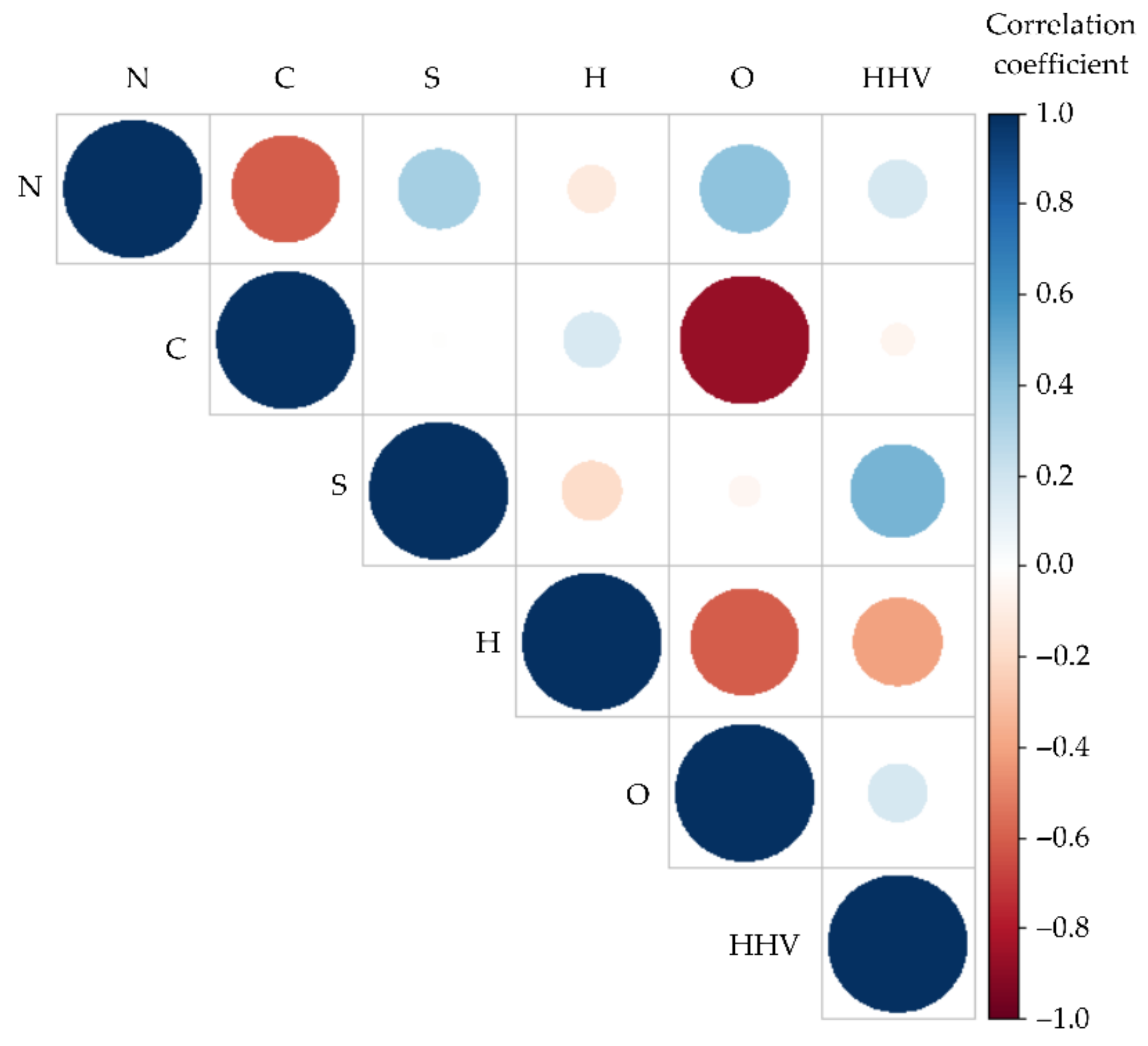
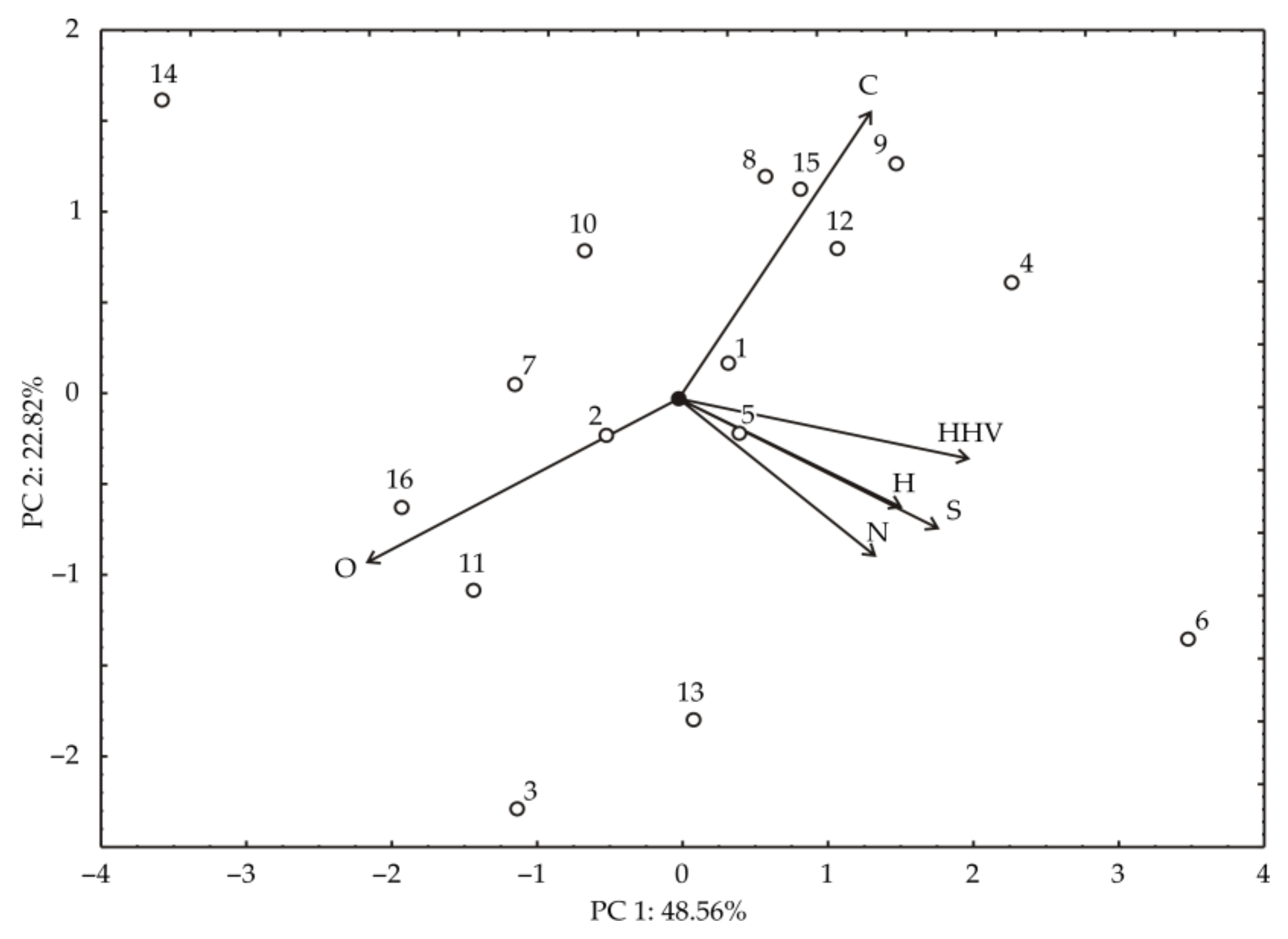
2.2. Statistical Analysis

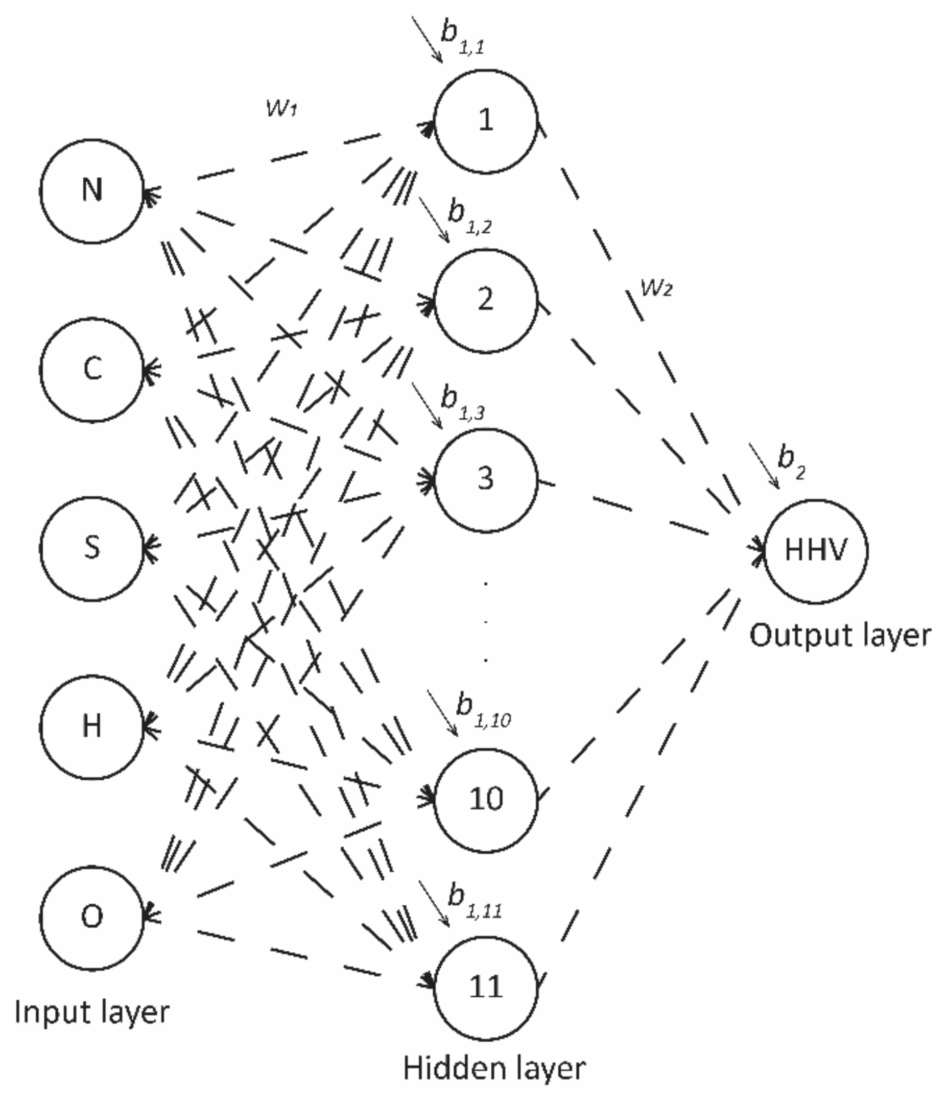
Statistical processing was performed using the software package TIBCO STATISTICA 13.3.0 (StatSoft TIBCO Software Inc., Palo Alto, CA, USA). The analyzed data are presented as means with standard deviation. Analysis of variance (ANOVA) with Tukey’s HSD post hoc test to compare sample means was used to examine variation in observed parameters.

To show the performance of the developed ANN model and predictive regression models for calculating HHV with ultimate analysis inputs (N, C, S, H, and O), it is necessary to calculate statistical parameters: reduced chi-square (x²) (Equation (1)), root mean square error (RMSE) (Equation (2)), coefficient of determination (R²), mean bias error (MBE) (Equation (3)), mean percentage error (MPE) (Equation (4)), and sum of squared estimate of errors (SSE) (Equation (5)). The RMSE shows the efficiency of the model by comparing the predicted values with the already measured values. The value obtained by the MBE is used as an indicator of the standard deviation of the predicted values from the measured values [19]. The listed parameters are given by the following formula [20].

$$x^2=\frac{{\displaystyle \sum _{i=1}^N(x_{pre,i}}-x_{\exp ,i}{)}^2}{N-n}$$

(1)

$$RMSE={\left[\frac{1}{N}·{\displaystyle \sum _{i=1}^N{(x_{pre,i}-x_{\exp ,i})}^2}\right]}^{1/2}$$

(2)

$$MBE=\frac{1}{N}\cdot {\displaystyle \sum _{i=1}^N(x_{pre,i}-x_{\exp ,i})}$$

(3)

$$MPE=\frac{100}{N}·{\displaystyle \sum _{i=1}^N\left(\frac{\left|x_{pre,i}-x_{\exp ,i}\right|}{x_{\exp ,i}}\right)}$$

(4)

$$SSE={\displaystyle \sum _{i=1}^N{(x_{pre,i}-x_{\exp ,i})}^2}$$

(5)

where x_exp,i stands for the experimental values and x_pre,i is the predicted values calculated by the model, N and n are the number of observations and constants, respectively.

Yoon’s method of global sensitivity (Equation (6)) was used to calculate the direct influence of the input parameters on the output variables, corresponding to the weighting coefficients within the ANN model [21]:

$$R{I}_{ij}(\%)=\frac{{\displaystyle \sum _{k=0}^n(w_{ik}\cdot w_{kj})}}{{\displaystyle \sum _{i=0}^m\left|{\displaystyle \sum _{k=0}^n(w_{ik}·w_{kj})}\right|}}·100\%$$

(6)

where w—denotes the weighting factor in the ANN model, i—input variable, j—output variable, k—hidden neuron, n—number of hidden neurons, m—number of inputs.

2.3. ANN Modeling

ANN are among the most researched areas of neurocomputing. A multilayer perceptron (MLP) is a neural network with hidden layers Figure 1. ANN can adapt its internal structure depending on the input data and the final goal of the function. The basic characteristics of ANN are the ability to learn independently, the ability to adapt the system to the available information and data processing, and to perform complex mathematical operations at high speed. The number of neurons and hidden layers in ANN can vary and is determined by the trial-and-error method [11]. Neural networks are categorized by their architecture, topology, and learning mode [22]. Neural networks take inputs, compute them, and convert them into outputs. This process is called the learning process of the network. The learning process of ANN can be supervised and unsupervised. In supervised learning mode, the model has access to output data for computations, while in unsupervised mode, there is no output data [23].

Models of ANN can provide a link between input and output data without using a complicated type of computational method. MLP ANN is recognized as the most effective type of ANN [9,24]. ANN is a mathematical structure developed from the motivation of the learning process in the human brain. ANN is a promising modeling technique for datasets with nonlinear relationships. Multilayer feedforward networks (MLP-ANN) consist of interdependent units (neurons). These neurons are arranged in the form of layers (input, hidden, and output layers). The number of neurons and hidden layers varies and can be determined by the method of trial and error so that the model error is minimal [11].

The data used for ANN were collected from the literature and were randomly divided into sets for training (70%), testing (15%) and validation (15%). ANN model was trained 100,000 times with a random number of hidden layers (1–20), and duration of creating the model was 27 min. The model was created on a computer with an Intel i5 processor (12th Gen Intel(R) Core(TM), i5-12400F, 2.50 GHz) and 8 GB of RAM.

Different transfer functions and random values for weighting coefficients and bias were used. Training of the network data was set up during the ANN learning cycle to determine the number of neurons and adjust the weight coefficients in each neuron [25]. The biases and weight coefficients related to the hidden and the output layers of the model are represented in the matrices and vectors W₁ and B₁ and W₂ and B₂, respectively [26]. The neural network model can be represented in matrix notation: Equation for calculating the output data (Equation (7)) of the neural network [27]:

$$Y=f_1(W_2\cdot f_2(W_1·X+B_1)+B_2)$$

(7)

where Y represents the output value, f₁ and f₂ represent the transfer function in the hidden and output layer, X represents the matrix of the input layer [28].

The Broyden-Fletcher-Goldfarb-Shanno (BFGS) algorithm was used for the calculations. The BFGS algorithm is one of the most effective algorithms for optimization and can be successfully used for the optimization of multivariate problems [29].

2.4. Regression Models

Table 1. List of equations for calculating HHV.

Sr.no.	Proposed Equations from the Literature	References
1	HHV = a + b · C	[31]
2	HHV − a + b · H	[31]
3	HHV − a + b · O	[31]
4	$HHV=a+b\cdot \frac{O}{C}$	[31]
5	$HHV=a+b\cdot \frac{H}{C}$	[31]
6	HHV = a + b · C + c · H + d · C2 + e · H2	[31]
7	$HHV=a+b\cdot \frac{O}{C}+c\cdot \frac{H}{C}+d\cdot {\left(\frac{O}{C}\right)}^2+e\cdot {\left(\frac{H}{C}\right)}^2$	[31]
8	HHV = a · C − b	[5]
9	HHV = a + b · C2 + c · C + d · H + e · C · H + g · N	[30]
10	$HHV=a+b\cdot {\left(C\right)}^2$	[31]

presents the models of the proposed equations for the calculation of HHV biomass found in the literature [5,30,31]. The models are based on establishing relations between variables based on ultimate analysis and HHV output values.

3. Results

Table 2. Average values of nitrogen, carbon, sulfur, hydrogen, and oxygen of investigated biomass of miscanthus.

Sample	N	C	S	H	O	HHV
MxG1	0.24 ± 0.15 a	51.49 ± 0.58 a	0.11 ± 0.04 a	5.82 ± 0.32 a	42.33 ± 0.74 a	18.21 ± 0.54 a
MxG2	0.19 ± 0.13 a	51.3 ± 0.53 a	0.14 ± 0.06 a	5.85 ± 0.2 a	42.53 ± 0.42 a	18.16 ± 0.37 a
MxG3	0.23 ± 0.15 a	50.9 ± 0.96 a	0.14 ± 0.06 a	5.82 ± 0.2 a	42.91 ± 0.89 a	18.22 ± 0.58 a
MxG4	0.22 ± 0.13 a	51.75 ± 0.73 a	0.21 ± 0.3 a	5.83 ± 0.33 a	41.99 ± 0.69 a	18.24 ± 0.64 a
MxG5	0.2 ± 0.09 a	51.38 ± 0.8 a	0.14 ± 0.08 a	5.84 ± 0.33 a	42.44 ± 0.82 a	18.37 ± 0.48 a
MxG6	0.31 ± 0.21 a	51.53 ± 0.86 a	0.21 ± 0.2 a	5.89 ± 0.23 a	42.06 ± 0.88 a	18.45 ± 0.61 a
MxG7	0.2 ± 0.13 a	51.33 ± 0.93 a	0.12 ± 0.09 a	5.82 ± 0.33 a	42.54 ± 0.92 a	17.97 ± 0.73 a
MxG8	0.2 ± 0.11 a	51.65 ± 1.33 a	0.11 ± 0.06 a	5.88 ± 0.27 a	42.16 ± 1.18 a	18.23 ± 0.64 a
MxG9	0.21 ± 0.12 a	51.76 ± 0.77 a	0.13 ± 0.05 a	5.85 ± 0.35 a	42.05 ± 0.86 a	18.35 ± 0.32 a
MxG10	0.18 ± 0.1 a	51.48 ± 0.97 a	0.11 ± 0.05 a	5.83 ± 0.33 a	42.4 ± 0.85 a	18.1 ± 0.61 a
MxG11	0.22 ± 0.16 a	51.09 ± 1.14 a	0.11 ± 0.05 a	5.85 ± 0.27 a	42.74 ± 1.12 a	18.06 ± 0.33 a
MxG12	0.19 ± 0.11 a	51.6 ± 0.82 a	0.12 ± 0.06 a	5.86 ± 0.35 a	42.24 ± 0.97 a	18.51 ± 0.5 a
MxG13	0.27 ± 0.22 a	51.15 ± 0.8 a	0.15 ± 0.09 a	5.79 ± 0.36 a	42.64 ± 0.86 a	18.24 ± 0.6 a
MxG14	0.2 ± 0.14 a	51.53 ± 0.82 a	0.09 ± 0.03 a	5.31 ± 1.71 a	42.86 ± 2.12 a	17.83 ± 0.81 a
MxG15	0.25 ± 0.15 a	51.73 ± 0.99 a	0.12 ± 0.05 a	5.83 ± 0.38 a	42.08 ± 1.19 a	18.09 ± 0.4 a
MxG16	0.18 ± 0.12 a	51.11 ± 1.12 a	0.11 ± 0.05 a	5.83 ± 0.33 a	42.77 ± 1.15 a	18.02 ± 0.43 a

N—Nitrogen (%); C—Carbon (%); S—Sulfur (%); H—Hydrogen (%); O—Oxygen (%). The means in the same row (various samples), with different lowercase superscripts, are statistically different (p ≤ 0.05), according to Tukey’s HSD test.

shows the mean values of the variables of the ultimate analysis and HHV with standard deviation and Tukey’s HSD test of miscanthus.

Table 2 shows the differences in the percentages of nitrogen, carbon, hydrogen, sulfur, and oxygen and is expressed as mean and standard deviation. The prefabricated statistical analysis shows that the observed values between the samples are not statistically significant (statistically significant at p ≤ 0.05). Higher content of C and H components leads to a higher total value of HHV [32]. The sample MxG 6 has the highest average content of N (0.31%) and H (5.89%) and a higher value of HHV (18.45 MJ/kg). The sample MxG 14 has the lowest average percentage value of elements S (0.09%) and H (5.31%) and the lowest value of HHV (17.83 MJ/kg). The average values in the paper are: 0.22% N, 51.42% C, 0.13% S, 5.80% H, 42.42% O and 18.18 MJ/kg for HHV.

The correlation analysis of the parameters of ultimate analysis and HHV was performed via Rstudio and related packages (corrplot).

The diagram of the correlation matrix shows the correlation coefficients between the variables. Positive values of the correlation coefficient are shown in blue, while negative values are shown in red. The intensity of the color in the circle is proportional to the correlation coefficient. In Figure 2, it can be observed that the elements O, S, and N are positively correlated with the value of HHV, while C and H are negative. It can be seen that variable S has the highest positive correlation coefficient, i.e., a significant influence on HHV, while variables N and O also have positively correlated values, but less influence on HHV. The variable H in the correlation graph shown has a negative correlation value on HHV. Based on Figure 2, HHV is best correlated with the concentrations of H, S, and N (when the blue color is shown, it is a positive correlation).

After determining the mean of all parameters, the correlations of the variables and their contribution were determined. The influence of the variables (N, C, S, H, O, and HHV) and the samples are combined graphically.

Principal Component Analysis (PCA) is used in the search for orthogonal directions of greatest dispersion of given data with the task of finding patterns in the distribution of individual data with respect to the original data defined in a space with multiple dimensions [33]. The analysis is also used to build predictive models, and it is easy to interpret the impact of individual variables on a given value. In Figure 3, the right side of the diagram shows sample 6, which is significant and has the highest values for HHV, H, N, and S. The upper part of the diagram shows samples 9, 8, 12, 15, 4 with the highest content of C. On the left side of the diagram are samples 14, 16, 11, 3, which have the highest content of O. According to the PCA analysis, the parameters N, S, H and HHV have the greatest influence on the data.

4. Discussion

4.1. Prediction of HHV Using Developed Regression Models

Table 3. Statistical test goodness of fit (developed regression models).

Model	x2	RMSE	MBE	MPE	SSE	R2	Skewness	Kurtosis	SD	Variance
Model 1	0.31	0.01	0.01	854.24	59.66	0.00	−0.63	1.47	0.56	0.31
Model 2	0.19	0.01	0.01	578.45	35.56	0.40	−1.32	9.26	0.43	0.19
Model 3	0.30	0.01	0.01	810.35	57.95	0.03	−0.67	2.10	0.55	0.30
Model 4	0.31	0.01	0.01	830.08	58.92	0.02	−0.65	1.81	0.56	0.31
Model 5	0.19	0.01	0.01	623.98	36.77	0.38	−1.19	6.78	0.44	0.19
Model 6	0.22	0.01	0.01	582.07	42.91	0.36	−1.53	12.54	0.47	0.22
Model 7	0.19	0.01	0.01	585.55	35.77	0.40	−1.28	8.67	0.43	0.19
Model 8	0.31	0.01	0.01	854.24	59.66	0.00	−0.63	1.47	0.56	0.31
Model 9	0.17	0.01	0.01	526.96	31.57	0.47	−1.79	13.09	0.41	0.17
Model 10	0.31	0.01	0.01	853.32	59.64	0.00	−0.63	1.49	0.56	0.31
ANN	0.07	0.27	-0.03	1.10	13.74	0.77	0.53	2.29	0.27	0.07

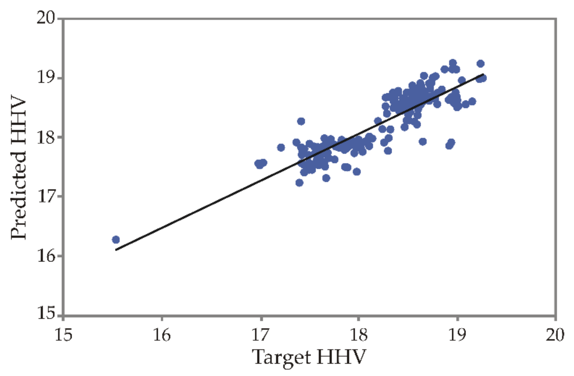
x²—reduced chi-square, RMSE—root mean square error, R²—coefficient of determination, MBE—mean bias error and MPE—mean percentage error, ANN—artificial neural network.

shows the calculated statistical test of “goodness of fit” for the proposed models to calculate the HHV value based on ultimate analysis.

The regression models offered from the literature use a different number of input variables of the ultimate analysis. Models 1,2,3,8,10 use one, while models 4,5,6 use two input variables. The highest number of input data is used by regression models 7 and 9, where the number of input variables is three. In contrast to the equations offered to calculate the HHV, ANN uses all five input variables of the ultimate analysis and shows the highest accuracy in prediction. The presented models in the calculations did not show sufficient accuracy and precision to be used as a reliable method for predicting HHV biomass of miscanthus. The coefficient of determination (R²) was used as the most important statistical parameter to evaluate the suitability of the mathematical models, which was lowest for model 1, 8 and model 10 (R² = 0.00) and highest for model 9 (R² = 0.47) in the calculations for 10 different models. The reliability of the regression models and ANN is ensured by the parameters MPE, SSE and R², but other parameters (for most models) also show good performance. The calculated statistical parameter x² shows good performance in models 2,5,7 (0.19) and in model 9 (0.17). For the above-mentioned reason, it is necessary to consider several statistical parameters when evaluating performance of the model.

4.2. ANN Model

In developing the model ANN, the input variables (N, C, S, H, and O) and the output value (HHV) had to be determined. The weights and biases were determined randomly by looking for values that would make the model accurate enough to predict the output.

The ANN model developed for the prediction of HHV showed a good ability to generalize data and predict. The model showed the best performance with 11 neurons in the hidden layer within the network, where a high R² value (0.77 overall) and an overall low sum of squares value (SOS) were achieved during the training cycle (

Table 4. Weights and biases of input and output layer.

Input Layer						Output Layer
Weight					Bias	Weight	Bias
N	C	S	H	O		HHV
−1.74	10.34	−30.08	−7.41	1.90	1.62	−1.76	2.06
−0.28	3.37	1.69	2.99	−4.61	−0.37	1.18
2.58	−0.83	−5.02	−0.40	−0.37	−1.56	0.20
4.23	−0.73	−6.78	−0.79	0.10	−1.40	−0.31
10.55	−3.52	−15.48	12.93	−0.96	−2.58	−1.91
1.08	1.54	1.49	−2.03	−3.48	−1.57	−0.44
3.56	−2.75	−8.74	1.54	1.03	−2.09	−1.30
−3.67	1.30	2.92	2.02	−2.74	−0.87	0.48
−2.72	−0.49	6.47	−0.49	0.34	0.75	−0.60
2.25	2.01	6.90	−5.15	1.20	3.20	0.47
−1.14	1.93	2.53	0.98	−1.49	0.71	−1.56

).

MLP-ANN (Multi-layer perceptron Artificial neural network) is one of the forms of ANN that are mostly used in applications for solving nonlinear equations [34]. Table 4 shows the weight coefficients and biases of the developed MLP-ANN network model. It can be seen that the best results were obtained with a hidden layer with a number of 11 hidden neurons, where the experimental values of HHV best match the values of HHV calculated with the ANN model.

Table 5. Summary of ANN.

Net. Name	Train. Perf.	Test Perf.	Valid. Perf.	Train. Error	Test Error	Valid. Error	Train. Algorithm	Error Function	Hidden Activation	Output Activation
MLP 5-11-1	0.861	0.902	0.951	0.042	0.026	0.021	BFGS 71	SOS	Tanh	Logistic

Train.—Training; Perf.—Performance; Valid.—Validation.

shows the training, test and validation performance of the model ANN, expressed by the coefficient of correlation and by the training (0.042), test (0.026), and validation (0.021) error of the model. Table 3 shows the results of the statistical test indicating the deviations between the observed values and the expected values. The values shown indicate the ability of the algorithm to predict according to the given model data.

Therefore, the ANN structural model MLP 5-11-1 proved to be sufficiently accurate to predict HHV based on the N, C, S, H, and O contents. The training (0.861), test (0.902) and validation (0.951) performance values shows that the model is able to predict values almost equal to the measured values.

Scatterplot is one of the most common visualization techniques, and displays and displays the behavior of the entered data [35,36]. Figure 4. shows the data of the predicted HHV versus the target HHV, which largely shows the overlap.

The calculated parameters comprising the statistical test “goodness of fit” are shown in Table 3. The reported values of x² (0.07), RMSE (0.27), MBE (−0.03), MPE (1.10), SSE (13.74), and R² (0.77). The residual analysis also yielded the parameters skewness (0.534), kurtosis (2.293), standard deviation (0.269), and variance (0.072). Conducted analysis shows that the model has good predictive accuracy.

The range in which the relevance factor is determined is between −1 and +1. The increase of HHV is mainly influenced by the increase of the parameter S. The influence of input variables was studied according to Yoon’s interpretation method for parameters N, C, S, H, O. In Figure 5 is the influence of variables N (−20.64%), C (3.13%), S (68.89%), H (−3.07%), and O (−4.27%) on the target value of HHV. In Figure 5, it can be seen that the parameters C and S have positive values of relative importance for the variable HHV, while the values of N, H, and O have a negative influence and are not factors of relative importance in determining the value of HHV. Looking at the calculation of the input data carried out according to Yoon’s method of interpretation based on the ultimate analysis the positive variable S have the greatest influence on the determination of the output values of HHV.

The predictive regression models offered in the literature are used as nonlinear models to predict HHV biomass of miscanthus. As shown in the paper, the use of the predictive models does not provide suitability and sufficient accuracy in determining the HHV miscanthus with respect to the input parameters. Using ANN as a nonlinear model to determine the HHV value provides a more convenient way of prediction and provides more accurate weighting coefficients and biases, which are the basis for establishing relations between input parameters and output data.

5. Conclusions

The use of ANN models to predict the energy properties of biomass has been increasingly explored recently. The main point of the study is the creation of an improved model (in the form of ANN) compared to existing literature regression models, as evidenced by a higher R² value. The calculations performed according to the proposed non-linear mathematical models are not suitable enough to predict the HHV biomass of miscanthus (R² ≤ 0.47). Incorporating available data from the ultimate analysis of miscanthus the developed neural network model showed high accuracy in predicting the higher heating value (overall R² = 0.77). The factors N, C, S, H, and O influence the value of HHV. In the developed model, the increase in HHV is mainly influenced by the increase in the values of the parameter S. Although these models are not yet widely used as mathematical models for prediction (especially for variables that have nonlinear relationships), they offer the possibility of obtaining the desired result with less time, lower cost, and satisfactory accuracy, which can replace existing empirical methods. The developed model will be able to make more accurate predictions as more input data is collected. Future plans are to expand the database (literature sources and experimental data) and the development of new models such as Random Forest Regression and Support Vector Machine.

References

1. Koçar, G.; Civaş, N. An overview of biofuels from energy crops: Current status and future prospects. Renew. Sustain. Energy Rev. 2013, 28, 900–916. [Google Scholar] [CrossRef]
2. Long, H.; Li, X.; Wang, H.; Jia, J. resources and their bioenergy potential estimation: A review. Renew. Sustain. Energy Rev. 2013, 26, 344–352. [Google Scholar] [CrossRef]
3. Baxter, X.C.; Darvell, L.I.; Jones, J.M.; Barraclough, T.; Yates, N.E.; Shield, I. Miscanthus combustion properties and variations with Miscanthus agronomy. Fuel 2014, 117, 851–869. [Google Scholar] [CrossRef] [Green Version]
4. Yi, L.; Feng, J.; Qin, Y.H.; Li, W.Y. Prediction of elemental composition of coal using proximate analysis. Fuel 2017, 193, 315–321. [Google Scholar] [CrossRef]
5. Sheng, C.; Azevedo, J.L.T. Estimating the higher heating value of biomass fuels from basic analysis data. Biomass Bioenergy 2005, 28, 499–507. [Google Scholar] [CrossRef]
6. Dai, Z.; Chen, Z.; Selmi, A.; Jermsittiparsert, K.; Denić, N.M.; Nešić, Z. Machine learning prediction of higher heating value of biomass. Biomass Convers. Biorefin. 2021, 1–9. [Google Scholar] [CrossRef]
7. Giwa, S.O.; Adekomaya, S.O.; Adama, K.O.; Mukaila, M.O. Prediction of selected biodiesel fuel properties using artificial neural network. Front. Energy 2015, 9, 433–445. [Google Scholar] [CrossRef]
8. Dashti, A.; Noushabadi, A.S.; Raji, M.; Razmi, A.; Ceylan, S.; Mohammadi, A.H. Estimation of biomass higher heating value (HHV) based on the proximate analysis: Smart modeling and correlation. Fuel 2019, 257, 115931. [Google Scholar] [CrossRef]
9. Pattanayak, S.; Loha, C.; Hauchhum, L.; Sailo, L. Application of MLP-ANN models for estimating the higher heating value of bamboo biomass. Biomass Convers. Biorefin. 2021, 11, 2499–2508. [Google Scholar] [CrossRef]
10. Vardiambasis, I.O.; Kapetanakis, T.N.; Nikolopoulos, C.D.; Trang, T.K.; Tsubota, T.; Keyikoglu, R.; Khataee, A.; Kalderis, D. Hydrochars as emerging biofuels: Recent advances and application of artificial neural networks for the prediction of heating values. Energies 2020, 13, 4572. [Google Scholar] [CrossRef]
11. Özveren, U. An artificial intelligence approach to predict gross heating value of lignocellulosic fuels. J. Energy Inst. 2017, 90, 397–407. [Google Scholar] [CrossRef]
12. Olatunji, O.O.; Akinlabi, S.; Madushele, N.; Adedeji, P.A.; Felix, I. Multilayer perceptron artificial neural network for the prediction of heating value of municipal solid waste. AIMS Energy 2019, 7, 944–956. [Google Scholar] [CrossRef]
13. Kartal, F.; Özveren, U. A deep learning approach for prediction of syngas lower heating value from CFB gasifier in Aspen plus®. Energy 2020, 209, 118457. [Google Scholar] [CrossRef]
14. Ahmed, A.A.M. Prediction of dissolved oxygen in Surma River by biochemical oxygen demand and chemical oxygen demand using the artificial neural networks (ANNs). J. King Saud Univ. Eng. Sci. 2017, 29, 151–158. [Google Scholar] [CrossRef] [Green Version]
15. Alizadeh, M.J.; Kavianpour, M.R. Development of wavelet-ANN models to predict water quality parameters in Hilo Bay, Pacific Ocean. Mar. Pollut. Bull. 2015, 98, 171–178. [Google Scholar] [CrossRef]
16. Noushabadi, A.S.; Dashti, A.; Ahmadijokani, F.; Hu, J.; Mohammadi, A.H. Estimation of higher heating values (HHVs) of biomass fuels based on ultimate analysis using machine learning techniques and improved equation. Renew. Energy 2021, 179, 550–562. [Google Scholar] [CrossRef]
17. Voća, N.; Leto, J.; Karažija, T.; Bilandžija, N.; Peter, A.; Kutnjak, H.; Šurić, J.; Poljak, M. Energy properties and biomass yield of miscanthus x giganteus fertilized by municipal sewage sludge. Molecules 2021, 26, 4371. [Google Scholar] [CrossRef] [PubMed]
18. Meehan, P.G.; Finnan, J.M.; Donnell, K.P.M. The effect of harvest date and harvest method on the combustion characteristics of Miscanthus X giganteus. GCB Bioenergy 2013, 5, 487–496. [Google Scholar] [CrossRef]
19. Khalil, S.A.; Shaffie, A.M. A comparative study of total, direct and diffuse solar irradiance by using different models on horizontal and inclined surfaces for Cairo, Egypt. Renew. Sustain. Energy Rev. 2013, 27, 853–863. [Google Scholar] [CrossRef]
20. Arsenović, M.; Pezo, L.; Stanković, S.; Radojević, Z. Factor space differentiation of brick clays according to mineral content: Prediction of final brick product quality. Appl. Clay Sci. 2015, 115, 108–114. [Google Scholar] [CrossRef]
21. Yoon, Y.; Swales, G.; Margavio, T.M. A Comparison of Discriminant Analysis versus Artificial Neural Networks. J. Oper. Res. Soc. 1993, 44, 51–60. [Google Scholar] [CrossRef]
22. Mesroghli, S.; Jorjani, E.; Chehreh Chelgani, S. Estimation of gross calorific value based on coal analysis using regression and artificial neural networks. Int. J. Coal Geol. 2009, 79, 49–54. [Google Scholar] [CrossRef]
23. Cinar, A.C. Training Feed-Forward Multi-Layer Perceptron Artificial Neural Networks with a Tree-Seed Algorithm. Arab. J. Sci. Eng. 2020, 45, 10915–10938. [Google Scholar] [CrossRef]
24. Darvishan, A.; Bakhshi, H.; Madadkhani, M.; Mir, M.; Bemani, A. Application of MLP-ANN as a novel predictive method for prediction of the higher heating value of biomass in terms of ultimate analysis. Energy Source Part A 2018, 40, 2960–2966. [Google Scholar] [CrossRef]
25. Grieu, S.; Faugeroux, O.; Traoré, A.; Claudet, B.; Bodnar, J.L. Artificial intelligence tools and inverse methods for estimating the thermal diffusivity of building materials. Energy Build. 2011, 43, 543–554. [Google Scholar] [CrossRef] [Green Version]
26. Voca, N.; Pezo, L.; Peter, A.; Suput, D.; Loncar, B.; Kricka, T. Modelling of corn kernel pre-treatment, drying and processing for ethanol production using artificial neural networks. Ind. Crop. Prod. 2021, 162, 113293. [Google Scholar] [CrossRef]
27. Pezo, L.L.; Ćurčić, B.L.; Filipović, V.S.; Nićetin, M.R.; Koprivica, G.B.; Mišljenović, N.M.; Lević, L.B. Artificial neural network model of pork meat cubes osmotic dehydratation. Hem. Ind. 2013, 67, 465–475. [Google Scholar] [CrossRef]
28. Kollo, T.; von Rosen, D. Advanced Multivariate Statistics with Matrices; Springer: Dordrecht, The Netherlands, 2005. [Google Scholar]
29. Garijo, D. A Bernstein Broyden–Fletcher–Goldfarb–Shanno collocation method to solve non-linear beam models. Int. J. Nonlinear Mech. 2021, 131, 103672. [Google Scholar] [CrossRef]
30. Nhuchhen, D.R.; Afzal, M.T. HHV predicting correlations for torrefied biomass using proximate and ultimate analyses. Bioengineering 2017, 4, 7. [Google Scholar] [CrossRef] [Green Version]
31. Callejón-Ferre, A.J.; Velázquez-Martí, B.; López-Martínez, J.A.; Manzano-Agugliaro, F. Greenhouse crop residues: Energy potential and models for the prediction of their higher heating value. Renew. Sustain. Energy Rev. 2011, 15, 948–955. [Google Scholar] [CrossRef]
32. Bilandžija, N.; Voća, N.; Leto, J.; Jurišić, V.; Grubor, M.; Matin, A.; Krička, T. Yield and Biomass Composition of Miscanthus x Giganteus in the Mountain Area of Croatia. In Transactions of FAMENA; University of Zagreb: Zagreb, Croatia, 2018; Volume 42, pp. 51–60. [Google Scholar]
33. Rutledge, D.N. Comparison of Principal Components Analysis, Independent Components Analysis and Common Components Analysis. J. Anal. Test. 2018, 2, 235–248. [Google Scholar] [CrossRef]
34. Agahian, S.; Akan, T. Battle royale optimizer for training multi-layer perceptron. Evol. Syst. 2021, 123456789. [Google Scholar] [CrossRef]
35. Geladi, P.; Manley, M.; Lestander, T. Scatter plotting in multivariate data analysis. J. Chemometr. 2003, 17, 503–511. [Google Scholar] [CrossRef]
36. Keim, D.A.; Hao, M.C.; Dayal, U.; Janetzko, H.; Bak, P. Generalized scatter plots. Inform. Visual. 2010, 9, 301–311. [Google Scholar] [CrossRef]
Figure 1. Structure of 5-11-1 ANN.
Mathematics 10 03732 g001
Figure 2. Correlation plot of observed values.
Mathematics 10 03732 g002
Figure 3. PCA of observed values.
Mathematics 10 03732 g003
Figure 4. Predicted HHV vs. target HHV.
Mathematics 10 03732 g004
Figure 5. Relative importance of variables on HHV.
Mathematics 10 03732 g005