Precorrected-FFT Accelerated Singular Boundary Method for High-Frequency Acoustic Radiation and Scattering

Abstract

This paper presents a precorrected-FFT (pFFT) accelerated singular boundary method (SBM) for acoustic radiation and scattering in the high-frequency regime. The SBM is a boundary-type collocation method, which is truly free of mesh and integration and easy to program. However, due to the expensive CPU time and memory requirement in solving a fully-populated interpolation matrix equation, this method is usually limited to low-frequency acoustic problems. A new pFFT scheme is introduced to overcome this drawback. Since the models with lots of collocation points can be calculated by the new pFFT accelerated SBM (pFFT-SBM), high-frequency acoustic problems can be simulated. The results of numerical examples show that the new pFFT-SBM possesses an obvious advantage for high-frequency acoustic problems.

1. Introduction

Acoustic radiation and scattering problems arise in many real-life applications, such as radar, sonar, non-destructive testing, and noise barrier, just to mention a few. In most cases, however, the acoustic problems are not solvable analytically, thus numerical methods are of considerable interest [1,2,3]. For numerical calculation, the discretization techniques are usually employed to discretize the computational domain or the boundary to elements or nodes. Therefore, the numerical methods can be broadly split into two basic types: the domain-discretization and the boundary-discretization methods.

In the domain-discretization methods, such as the finite element method (FEM) [4], the perfectly matched layers usually should be introduced, since the sound waves always propagate in the unbound domain. By comparison, in some boundary-discretization methods, such as the boundary element method (BEM) [5], the method of fundamental solutions (MFS) [6], and the singular boundary method (SBM) [7], the special treatment for the infinite domain is usually not required, because the fundamental solutions are adopted as the kernel function, and the conditions at infinity are satisfied automatically. Furthermore, one dimension is reduced in the boundary-type methods. Therefore, they are more suitable to simulate exterior acoustic problems. The singular boundary method (SBM) is a strong-form boundary collocation method, which avoids mesh-generation and elemental interpolation in the BEM. The core idea of the SBM is that the finite values, which are called original intensity factors (OIFs), are introduced to desingularize the source singularities of the fundamental solutions. Therefore, the troublesome choice of an optimal fictitious boundary in the MFS is avoided. Therefore, it is a competitive alternative to acoustic problems [8,9]. Furthermore, it has successfully been employed to deal with some other physical problems [10,11,12,13].

However, the fully populated interpolation matrices are generated in the SBM. For large dense linear systems, the computational cost is expensive. If the direct solver Gaussian elimination is employed, $O\left(N^3\right)$ operations and $O\left(N^2\right)$ memory are required, where N is the number of the boundary points. If the iterative solvers, such as generalized minimal residual algorithm (GMRES) [14], are employed, the operations could be reduced to $O\left(N^2\right)$. However, for large-scale high-frequency acoustic wave problems, the interpolation matrices are also highly ill-conditioned. It brings not only the huge computational cost in each iteration, but also a large number of iteration steps. Consequently, the application of the SBM is restricted to small-scale and low-frequency problems.

Some fast algorithms, including the fast multipole method (FMM) [15], the adaptive cross approximation (ACA) [16], and the pFFT technique [17] have been employed to deal with the computational bottlenecks in the SBM. Compared with the other methods, the implement of the pFFT technique is easier and relatively independent from the kernel functions. The pFFT-SBM has been successfully employed to potential and Helmholtz problems. A new pFFT-SBM is developed in this study to solve high-frequency acoustic radiation and scattering. It should be noted that the pFFT scheme in this work is similar to the previous pFFT-SBM [18,19]. However, this study shows different ways to generate the interpolation, projection and convolution matrices, which require less memory and CPU time. The new scheme in this study can be easily expanded to more complicated problems, such as elastodynamic [20] and size-dependent elasticity [21,22]. The performance of the proposed method is investigated by numerical examples.

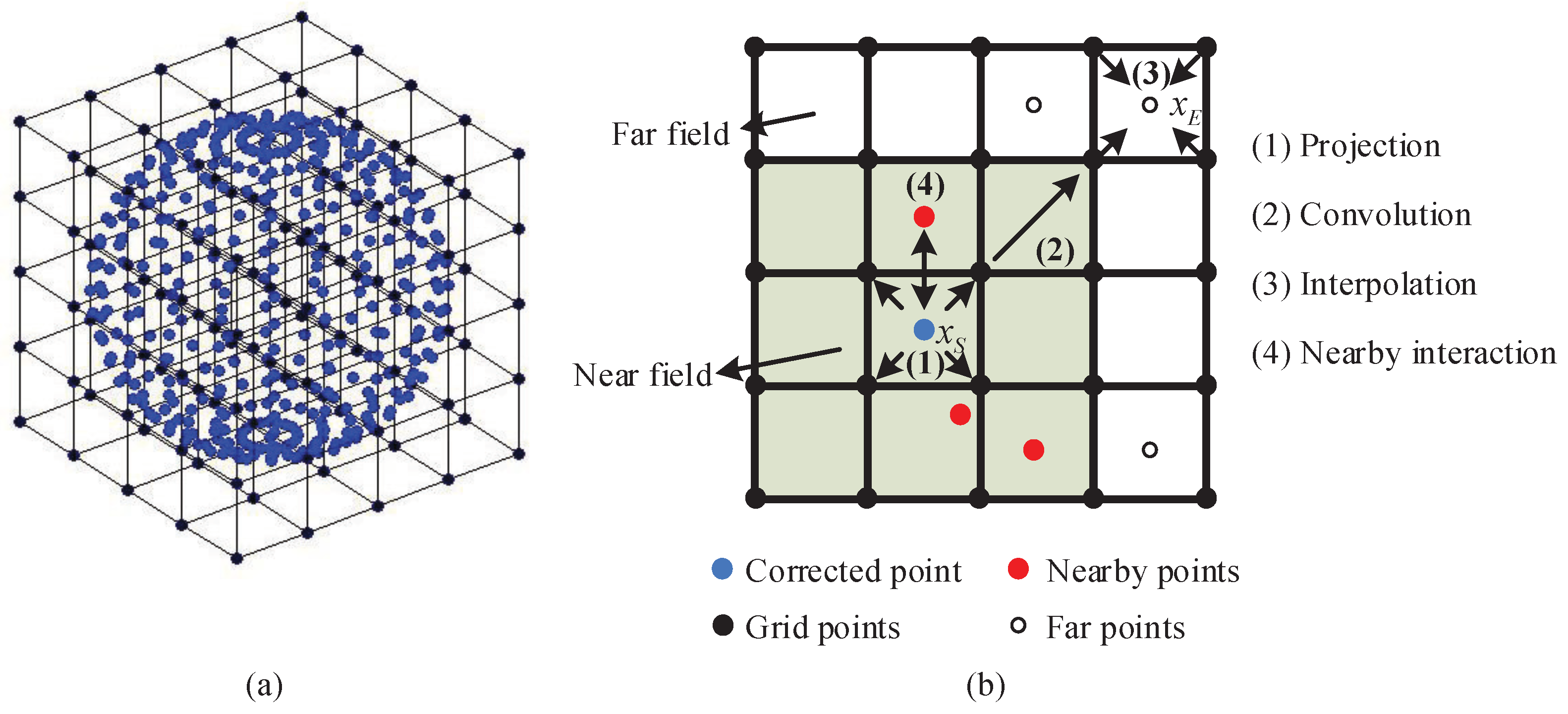
2. The pFFT-SBM Formulations for Acoustic Radiation and Scattering

We focus on the time-harmonic acoustic wave propagation in homogeneous isotropic media. The governing equation is the well-known Helmholtz equation [8]

$${\nabla }^{2}u\left(\mathit{x}\right)+k^{2}u\left(\mathit{x}\right)=0,\mathit{x}\in \mathsf{\Omega },$$

(1)

where $k=2\pi f/c$ is the wavenumber, f—the frequency, c—the acoustic wave speed, $\mathsf{\Omega }\in R^3$—the acoustic medium, and $u\left(\mathit{x}\right)$—the acoustic pressure of radiated or scattered waves on the boundary point $\mathit{x}$,

$$u=\left\{\begin{array}{cc}{u}_R=u_T,\hfill & \mathrm{for}\mathrm{radiation},\hfill \\ u_S=u_T-u_I,\hfill & \mathrm{for}\mathrm{scattering},\hfill \\ u_{R+S}=u_T-u_I,\hfill & \mathrm{for}\mathrm{both},\hfill \end{array}\right.$$

(2)

where the subscripts T, R, and I denote the total, radiation, and incidence waves, respectively. The boundary condition is Dirichlet type

$$u\left(\mathit{x}\right)=\overline{u}\left(\mathit{x}\right),\mathit{x}\in {\mathsf{\Gamma }}_D,$$

(3)

or Neumann type

$$q\left(\mathit{x}\right)=\frac{\partial u}{\partial \mathit{n}}\left(\mathit{x}\right)=\mathrm{i}\omega \rho \overline{v},\mathit{x}\in {\mathsf{\Gamma }}_N,$$

(4)

where $\overline{u}$ is the given acoustic pressure, $\mathit{n}=(n_x,n_y,n_z)$ the outward normal vector on the boundary point $\mathit{x}$, $\mathrm{i}=\sqrt{-1}$, $\omega =2\pi f$ the circular frequency, $\rho$ the density of the acoustic medium, $\overline{v}$ the normal velocity on the boundary, and $\mathsf{\Gamma }={\mathsf{\Gamma }}_D\cup {\mathsf{\Gamma }}_N=\partial \mathsf{\Omega }$ the whole physical boundary. Moreover, the acoustic pressure for exterior problems has to satisfy the following Sommerfeld radiation condition [8]

$$\underset{r\to \infty }{lim}\left(r\left[\frac{\partial u\left(r\right)}{\partial r}-\mathrm{i}ku\left(r\right)\right]\right)=0,$$

(5)

where $r={∥\mathit{x}∥}_2$.

For acoustic problems, the approximate solutions in the SBM can be expressed by utilizing the singular-layer fundamental solution, double-layer fundamental solution, or Burton–Miller’s formulation. According to the study in ref. [8], the singular-layer SBM (SL-SBM), double-layer SBM (DL-SBM), and Burton–Miller SBM (BM-SBM) have the same rapid convergence rate for 2D acoustic problems, however, the convergence speed of the SL-SBM is lower than the DL-SBM and BM-SBM for 3D problems. Moreover, the BM-SBM could overcome the nonuniqueness problem at certain characteristic frequencies for exterior acoustic problems in the SL-SBM and DL-SBM. In this study, we focus on the novel scheme of the pFFT and its performance in the SBM, therefore, the SL-SBM, whose form is the simplest, is employed. The development of the pFFT-SBM based on Burton–Miller’s formulation will be investigated in a subsequent paper.

In the SL-SBM, the approximate solutions can be expressed as [8]

$$u\left({\mathit{x}}_i\right)=\sum _{j=1,j\ne i}^N{\alpha }_{j}G({\mathit{x}}_i,{\mathit{y}}_j)+{\alpha }_i{U}^{ii},i=1,\cdots ,N,$$

(6)

$$q\left({\mathit{x}}_i\right)=\sum _{j=1,j\ne i}^N{\alpha }_j\frac{\partial G({\mathit{x}}_i,{\mathit{y}}_j)}{\partial \mathit{n}}+{\alpha }_i{Q}^{ii},i=1,\cdots ,N,$$

(7)

where ${\left\{{\alpha }_i\right\}}_{i=1}^N$, ${\left\{{\mathit{x}}_i\right\}}_{i=1}^N$ and ${\left\{{\mathit{y}}_i\right\}}_{i=1}^N$ are respectively the unknown coefficients, collocation and source points, N—the number of source points. $G({\mathit{x}}_i,{\mathit{y}}_j)$ is the fundamental solution given as

$$G({\mathit{x}}_i,{\mathit{y}}_j)=\frac{e^{\mathrm{i}k{∥{\mathit{x}}_i-{\mathit{y}}_i∥}_2}}{4\pi {∥{\mathit{x}}_i-{\mathit{y}}_i∥}_2},$$

(8)

and $U^{ii}$ and $Q^{ii}$ are OIFs that can be numerically calculated by [15]

$$U^{ii}=\frac{1}{L_i}{\int }_{S_i}G({\mathit{x}}_i,\mathit{y})d{S}_i,i=1,\cdots ,N,$$

(9)

$$Q^{ii}=\frac{\kappa }{2L_i}+\frac{1}{L_i}{\int }_{S_i}\frac{\partial G({\mathit{x}}_i,\mathit{y})d{S}_i}{\partial n},i=1,\cdots ,N,$$

(10)

where $\kappa =-1$ for exterior acoustic problems and $\kappa =1$ for interior acoustic problems, and $L_i$ indicates the area of integration cell $S_i$, which is the small influence domain surrounding the point ${\mathit{y}}_i$.

Based on Equations (6) and (7), a linear system of the equation can be obtained

$$\mathit{A}\mathit{\alpha }=\mathit{b},$$

(11)

where $\mathit{A}$ is the fully populated coefficient matrix, $\mathit{\alpha }$ the unknown vector, $\mathit{b}$ the boundary condition. The required memory usage of the coefficient matrix $\mathit{A}$ is of $O\left(N^2\right)$. If the iterative solver GMRES is employed, the computing operations for solving Equation (11) is of $O\left(N^2\right)$. To obtain acceptable results, the SBM needs about 6–7 points per wavelength in each direction. As the frequency of the acoustic problem grows, the number of required boundary points is increasing rapidly. Therefore, the scale of the linear system Equation (11) becomes huge, and it is difficult to be solved by the traditional GMRES. It is known that a matrix-vector production must be computed at each iteration of GMRES, and is the most time-consuming part of this solver. Thus, a new pFFT technique, which is a revised version of the original pFFT [18,19], is applied to accelerate the matrix-vector production.

Firstly, a uniform 3D grid should be constructed as shown in Figure 1a, and the problem domain is divided into an array of 3D small cubes that are equal-sized. The process of division can be adaptive until the number of boundary collocation points in each cube is less than a threshold value (typically 20). As shown in Figure 1b, the interaction computation is separated into two parts: near-field and far-field. With the help of the 3D grid, the far-field part (collocation points in nonadjacent cubes) is computed quickly, and the near-field part (collocation points in adjacent cubes) is calculated directly. Thus, the pFFT algorithm consists of four steps: projection, convolution, interpolation and nearby interaction.

Figure 1. The pFFT algorithm: (a) construction of the 3D uniform grid; (b) the four steps: 2D pictorial representation.

As an example, a 2D $4\times 4$ uniform grid in the near-field is considered as shown in Figure 1b. In the interpolation, a linear combination of simple polynomials is employed to compute the physical quantity $\phi (x,y)$ at any point $(x,y)$:

$$\phi (x,y)=\sum _k{c}_k{f}_k(x,y)={\mathit{f}}^T\mathit{c},$$

(12)

where ${\left\{c_k\right\}}_{k=0}^{16}$ is the coefficient, and the polynomials $f_k(x,y)$ are chosen as

$$f_k(x,y)=x^i{y}^j,i,j=0,1,2,3,k=2i+j,$$

(13)

Then, the following matrix form is obtained by matching $\phi (x,y)$ for each grid point

$${\mathit{\phi }}_g={\left[\begin{array}{cccc}{\phi }_{g,1}& {\phi }_{g,2}& \dots & {\phi }_{g,16}\end{array}\right]}^T=\mathit{Fc},$$

(14)

where ${\phi }_{g,j}$ is the given quantity at the j-th grid point $(x_j,y_j)$, and the j-th row of $\mathit{F}$ is the set of polynomial $\mathit{f}$ evaluated at point $(x_j,y_j)$. Based on Equations (12) and (14), we yield

$$\phi (x,y)={\mathit{f}}^T\mathit{c}={\mathit{f}}^T{\mathit{F}}^{-1}{\phi }_g={\mathit{I}}_0{\phi }_g.$$

(15)

where ${\mathit{I}}_0={\mathit{f}}^T{\mathit{F}}^{-1}$. The normal derivative of $\phi (x,y)$ can be yielded as

$$\frac{\partial \phi (x,y)}{\partial \mathit{n}}=\left(\frac{\partial {\mathit{f}}^T}{\partial x}{n}_x+\frac{\partial {\mathit{f}}^T}{\partial y}{n}_y\right)\mathit{c}=\left(\frac{\partial {\mathit{f}}^T}{\partial x}{n}_x+\frac{\partial {\mathit{f}}^T}{\partial y}{n}_y\right){\mathit{F}}^{-1}{\phi }_g={\mathit{I}}_n{\phi }_g,$$

(16)

where ${\mathit{I}}_n=\left(\frac{\partial {\mathit{f}}^T}{\partial x}{n}_x+\frac{\partial {\mathit{f}}^T}{\partial y}{n}_y\right){\mathit{F}}^{-1}$. Therefore, for each collocation point in the SBM, Equations (15) and (16) can be written as

$$\ell \left({\phi }^m\right)={\mathit{I}}_{\beta }^{\left(m\right)}{\phi }_g^{\left(m\right)},m=1,2,\cdots ,N,$$

(17)

where the operator ℓ is the identity operator or the operator $\partial (·)/\partial n$, and ${\mathit{I}}_{\beta }^{\left(m\right)}$ represents ${\mathit{I}}_0^{\left(m\right)}$ or ${\mathit{I}}_n^{\left(m\right)}$. The matrix format of Equation (17) is

$$\mathsf{\Psi }=\mathit{I}{\mathit{\phi }}_g,$$

(18)

where $\mathsf{\Psi }$ is the quantity or the normal vector at collocation points, and $\mathit{I}$ is the interpolation matrix.

The matrix form of the projection is

$${\mathit{Q}}_g=\mathit{Pv}={\mathit{I}}^T\mathit{v},$$

(19)

where ${\mathit{Q}}_g$ and $\mathit{v}$ are the total grid and collocation points charges, and $\mathit{P}$ is the projection matrix. It should be noticed that the interpolation and projection matrices are not related to the fundamental solution (8). Then, if the Helmholtz equation Equation (1) with different frequencies is calculated, these two matrices are only generated once. It shows an obvious advantage over the original pFFT.

The grid quantities can be calculated by the grid charges with the convolution matrix

$${\phi }_{g,j}=\sum _{i}G({\mathit{x}}_{g,i},{\mathit{x}}_{g,i})Q_{g,i},$$

(20)

or the matrix form

$${\mathit{\phi }}_g=\mathit{C}{\mathit{Q}}_g,$$

(21)

where $\mathit{C}$ is the convolution matrix. Due to the position invariant property of the fundamental solution, it can be known that $\mathit{C}$ is a multilevel Toeplitz matrix, and the production of it and a vector can be calculated by FFT quickly.

For the Dirichlet problems, the calculation of the convolution matrix $\mathit{C}$ in this study is the same as that in the original pFFT-SBM. However, there is a difference for the Neumann problems. In the original pFFT-SBM, when the convolution matrix is calculated, some special treatment has to be employed to deal with the operator $\partial (·)/\partial n$. Usually, it has to be done as follows

$$\frac{\partial G}{\partial \mathit{n}}=\frac{\partial G}{\partial x}{n}_x+\frac{\partial G}{\partial y}{n}_y+\frac{\partial G}{\partial z}{n}_z.$$

(22)

Therefore, three convolution matrices corresponding to $\frac{\partial G}{\partial x}$, $\frac{\partial G}{\partial y}$, and $\frac{\partial G}{\partial z}$ have to be generated. The FFT calculation has also to be carried out three times. In the study, the convolution matrix $\mathit{C}$ is only related to the fundamental solution (8), and the effect of the operator $\partial (·)/\partial n$ needs not to be considered. Hence, only one convolution matrix is calculated in the matrix-vector production. Then, more memory usage and CPU time are saved.

Substituting Equations (19) and (21) into (18) yields

$$\mathsf{\Psi }=\mathit{Av}=\mathit{ICPv}.$$

(23)

It implies

$$\mathit{A}=\mathit{ICP}.$$

(24)

Since the calculations of the near-field interaction by Equation (24) are inaccurate, they should be removed and the near-field interactions are computed directly. Then, the interaction in the near-field can be corrected as

$$E_{i,j}=A_{i,j}-{\mathit{I}}_i{\mathit{C}}_i{\mathit{P}}_j,i=1,2,\cdots ,N,j\in {\Xi }_i,$$

(25)

where $E_{i,j}$ is the element of the precorrected matrix, $A_{i,j}$ is the direct interaction defined in Equation (24) between the source point and its neighbors, ${\mathit{I}}_i$, ${\mathit{P}}_j$, and ${\mathit{C}}_i$ represent the sub-matrices of Equations (18), (19) and (21) corresponding to the i-th source points and ${\Xi }_i$, which is the set containing indices of the neighbor points for the i-th source point.

Then, Equation (24) is modified to

$$\mathit{A}=\mathit{E}+\mathit{ICP},$$

(26)

where $\mathit{E}$ is the precorrected direct matrix, in which the element is defined in Equation (25).

3. Numerical Examples

In this part, the non-dimensional wave number $kD$ is used, where D is the maximum diameter of the physical domain. To simulate the examples, both the traditional SBM and the new pFFT-SBM are used, and all the computations are performed on a desktop with a 2.40 GHz CPU and 4GB RAM. The following relative error formula is used

$$Error=\sqrt{\frac{1}{M}\sum _{k=1}^M{\left(\frac{I_{num}^k-I_{an}^k}{I_{an}^k}\right)}^2},$$

(27)

where M is the number of the test points, $I_{an}^k$ and $I_{num}^k$ are analytical and numerical solutions at the k-th test point, respectively. The tolerance of the iterative solver GMRES is set to $1.0\times {10}^{-3}$, and a sparse matrix preconditioner stored and LU factored by SuperLU [23] is also employed.

3.1. Scattering of a Plane Acoustic Wave by a Rigid Sphere

A rigid unit sphere center at (0, 0, 0) is considered as the first example. Assume the incident wave $u_{in}=e^{ikz}$ propagates along the positive z-axis, and the analytical solution of the scattering of the plane acoustic pressure can be given as

$$u(r,\theta )=\sum _{n=0}^{\infty }-{\mathrm{i}}^n(2n+1)\frac{n{j}_{n-1}\left(ka\right)-(n+1)j_{n+1}\left(ka\right)}{n{h}_{n-1}^{\left(1\right)}\left(ka\right)-(n+1)h_{n+1}^{\left(1\right)}\left(ka\right)}{h}_n^{\left(1\right)}\left(kr\right)P_n(cos\theta ),$$

(28)

where $j_n$ is the n-th order spherical Bessel function of the first kind, $h_n^{\left(1\right)}$ the n-th order Hankel function of the first kind, and $P_n$ the n-th Legendre polynomial.

The non-dimensional wave number is set to $kD=20.0$ ($D=2$, $f=541$ Hz). The relative errors of the traditional SBM and new pFFT-SBM are shown in Table 1. It can seen that the new pFFT-SBM almost keeps the accuracy of the traditional SBM. However, the traditional SBM is unavailable for the large-scale simulation, and the new pFFT-SBM still works well. The reason is that the required memory and its increasing rate of the new pFFT-SBM are significantly smaller than those of the traditional SBM, as shown in Figure 2. Figure 3 shows the comparison of the CPU time of these two methods. We can find that the CPU time of the new pFFT-SBM is also much smaller. For the model with 12,288 collocation points, only 16.92% memory usage and 4.11% computational time of the traditional SBM are required in the pFFT-SBM. Furthermore, the figures clearly show that the growth of the computational cost of the new pFFT-SBM is almost linearly with the number of collocation points. This numerical example demonstrates that the new pFFT-SBM is accurate, stable, and efficient, especially for large-scale acoustic problems.

Table 1. The relative errors of the traditional SBM and new pFFT-SBM for example 1.

Numbers of Points	768	3072	12,288	49,152	196,608
Traditional SBM	$3.80\times {10}^{-2}$	$2.05\times {10}^{-2}$	$1.07\times {10}^{-2}$	-	-
pFFT-SBM	$4.03\times {10}^{-2}$	$2.15\times {10}^{-2}$	$1.09\times {10}^{-2}$	$5.52\times {10}^{-2}$	$2.63\times {10}^{-2}$

Figure 2. Memory requirements versus the problem size for example 1.

Figure 3. Total CPU time versus the problem size for example 1.

3.2. Radiation from a Car

To further test the pFFT-SBM to a complex case, the second example deals with the problem of radiation from a car with a length of 4.1 m, a width of 2.0 m, and a height of 1.1 m, as shown in Figure 4. The analytical solution of the radiation field is

$$u=\frac{e^{ikr}}{r},$$

(29)

where $r=\sqrt{x^2+y^2+z^2}$.

Figure 4. The sketch of a car.

At first, a low-frequency case is considered. The non-dimensional wave number is set to $kD=7.58$ ($D=4.1$, $f=100$ Hz). The results of the traditional SBM and new pFFT-SBM are shown in Table 2. It shows that the accuracy and the convergence rate of the new pFFT-SBM are almost the same as those of the traditional SBM. Compared to the traditional SBM, the significant advantage of the new pFFT-SBM in saving computational cost is also very obvious in this table.

Table 2. The results of a low-frequency case of example 2 by the traditional SBM and pFFT-SBM.

Numbers of Points	Relative Error		CPU Time (s)		Memory
	Traditional SBM	pFFT-SBM	Traditional SBM	pFFT-SBM	Traditional SBM	pFFT-SBM
2106	$2.73\times {10}^{-2}$	$2.67\times {10}^{-2}$	119	28	82.7	65.3
13,154	$9.03\times {10}^{-3}$	$9.04\times {10}^{-3}$	5054	148	2676.4	133.5
51,252	-	$5.62\times {10}^{-3}$	-	634	-	628.3
144,128	-	$3.87\times {10}^{-3}$	-	2728	-	1372.1

Next, we consider a higher-frequency case. The non-dimensional wave number is set to $kD=50.0$ ($D=4.1$, $f=660$ Hz). A total of 144,128 boundary collocation points are distributed on the surface of the car. Based on this model, the pFFT-SBM takes 18,528 s to obtain the numerical results with an average relative error of 1.75%.

4. Conclusions

In this study, a new fast SBM based on the pFFT algorithm is developed for acoustic radiation and scattering in the high-frequency regime. The numerical examples show a significant advantage of the pFFT-SBM over the traditional SBM in saving the computational cost while the accuracy is maintained. Therefore, it can keep working well for high-frequency acoustic problems while the traditional SBM is inapplicable on a personal computer. It should be noted that the new scheme in this study can be easily expanded to more complicated kernels.

References

- Sun, Y.; Hao, S. A numerical study for the Dirichlet problem of the Helmholtz equation. Mathematics 2021, 9, 1953. [Google Scholar] [CrossRef]
- Cheng, H.; Peng, M. The improved element-free Galerkin method for 3D Helmholtz equations. Mathematics 2022, 10, 14. [Google Scholar] [CrossRef]
- Qu, W.; Gao, H.; Gu, Y. Integrating Krylov deferred correction and generalized finite difference methods for dynamic simulations of wave propagation phenomena in long-time intervals. Adv. Appl. Math. Mech. 2021, 13, 1398–1417. [Google Scholar]
- Chai, Y.; You, X.; Li, W. Dispersion reduction for the wave propagation problems using a coupled “FE-meshfree” triangular element. Int. J. Comput. Methods 2020, 17, 1950071. [Google Scholar] [CrossRef]
- Liu, Y. On the BEM for acoustic wave problems. Eng. Anal. Bound. Elem. 2019, 107, 53–62. [Google Scholar] [CrossRef]
- Cheng, A.H.D.; Hong, Y. An overview of the method of fundamental solutions–Solvability, uniqueness, convergence, and stability. Eng. Anal. Bound. Elem. 2020, 120, 118–152. [Google Scholar] [CrossRef]
- Chen, W. Singular boundary method: A novel, simple, meshfree, boundary collocation numerical method (in Chinese). Chin. J. Solid Mech. 2009, 30, 592–599. [Google Scholar]
- Fu, Z.; Chen, W.; Gu, Y. Burton-Miller-type singular boundary method for acoustic radiation and scattering. J. Sound Vib. 2014, 333, 3776–3793. [Google Scholar] [CrossRef]
- Lin, J.; Chen, W.; Chen, C.S. Numerical treatment of acoustic problem with boundary singularities by the singular boundary method. J. Sound Vib. 2014, 333, 3177–3188. [Google Scholar] [CrossRef]
- Li, W.; Chen, W. Band gap calculations of photonic crystals by the singular boundary method. J. Comput. Appl. Math. 2017, 315, 273–286. [Google Scholar] [CrossRef]
- Fu, Z.; Chen, W.; Wen, P.; Zhang, C. Singular boundary method for wave propagation analysis in periodic structures. J. Sound Vib. 2018, 425, 170–188. [Google Scholar] [CrossRef]
- Gu, Y.; Chen, W.; Zhang, C. Singular boundary method for solving plane strain elastostatic problems. Int. J. Solids Struct. 2011, 48, 2549–2556. [Google Scholar] [CrossRef] [Green Version]
- Li, W. Localized method of fundamental solutions for 2D harmonic elastic wave problems. Appl. Math. Lett. 2021, 112, 106759. [Google Scholar] [CrossRef]
- Saad, Y.; Schultz, M.H. GMRES: A Generalized Minimal Residual Algorithm for Solving Nonsymmetric Linear Systems. SIAM J. Sci. Stat. Comput. 1986, 7, 856–869. [Google Scholar] [CrossRef] [Green Version]
- Qu, W.; Chen, W.; Zhang, C. Diagonal form fast multipole singular boundary method applied to the solution of high-frequency acoustic radiation and scattering. Int. J. Numer. Meth. Eng. 2017, 111, 803–815. [Google Scholar] [CrossRef]
- Wei, X.; Chen, B.; Chen, S.; Yin, S. An ACA-SBM for some 2D steady-state heat conduction problems. Eng. Anal. Bound. Elem. 2016, 71, 101–111. [Google Scholar] [CrossRef]
- Phillips, J.R.; White, J.K. A precorrected-FFT method for electrostatic analysis of complicated 3-d structures. IEEE Trans. Comput. Aided Des. Integr. Circuits Syst. 1997, 16, 1059–1072. [Google Scholar] [CrossRef] [Green Version]
- Li, W. A fast singular boundary method for 3D Helmholtz equation. Comput. Math. Appl. 2019, 72, 525–535. [Google Scholar] [CrossRef]
- Li, W.; Chen, W. Precorrected-FFT accelerated singular boundary method for large-scale three-dimensional potential problems. Commun. Comput. Phys. 2017, 22, 460–472. [Google Scholar] [CrossRef]
- Qu, W.; He, H. A GFDM with supplementary nodes for thin elastic plate bending analysis under dynamic loading. Appl. Math. Lett. 2022, 124, 107664. [Google Scholar] [CrossRef]
- Faghidian, S.A. Contribution of nonlocal integral elasticity to modified strain gradient theory. Eur. Phys. J. Plus 2021, 136, 559. [Google Scholar] [CrossRef]
- Barretta, R.; Faghidian, S.A.; Sciarra, F.M.D. Aifantis versus Lam strain gradient models of Bishop elastic rods. Acta. Mech. 2019, 230, 2799–2812. [Google Scholar] [CrossRef]
- Li, X.S. An overview of SuperLU: Algorithms, implementation, and user interface. ACM Trans. Math. Softw. 2005, 31, 302–325. [Google Scholar] [CrossRef]
Publisher’s Note: MDPI stays neutral with regard to jurisdictional claims in published maps and institutional affiliations. |
© 2022 by the authors. Licensee MDPI, Basel, Switzerland. This article is an open access article distributed under the terms and conditions of the Creative Commons Attribution (CC BY) license (https://creativecommons.org/licenses/by/4.0/).