
On Asymptotics of Optimal Stopping Times


Abstract
:1. Introduction
2. Formulation
3. Computing Behaviour
3.1. Recurrence Relation for
3.2. Asymptotics of as
3.3. Example Calculations
3.4. Tabulation of Further Examples
4. Calculating Optimal Stopping Statistics
4.1. Calculating the Expectation
4.2. Calculating the Variance
4.3. Higher Moments
4.4. Example Calculations
5. Numerical Comparisons
6. Applications
7. Conclusions
Author Contributions
Funding
Institutional Review Board Statement
Informed Consent Statement
Data Availability Statement
Conflicts of Interest
References
- Ferguson, T.S. Who solved the secretary problem? Stat. Sci. 1989, 4, 282–296. [Google Scholar] [CrossRef]
- Seale, D.A.; Rapoport, A. Sequential Decision Making with Relative Ranks: An Experimental Investigation of the “Secretary Problem”. Organ. Behav. Hum. Decis. Process. 1997, 69, 221–236. [Google Scholar] [CrossRef]
- Stein, W.E.; Seale, D.A.; Rapoport, A. Analysis of heuristic solutions to the best choice problem. Eur. J. Oper. Res. 2003, 151, 140–152. [Google Scholar] [CrossRef]
- David, I. Explicit results for a class of asset-selling problems. Eur. J. Oper. Res. 1998, 110, 576–584. [Google Scholar] [CrossRef]
- Karlin, S. Stochastic models and optimal policy for selling an asset. In Studies in Applied Probability and Management Science; K. J. Arrow, S.K., Scarf, H., Eds.; Stanford University Press: Stanford, CA, USA, 1962. [Google Scholar]
- Sofronov, G.Y. An Optimal Decision Rule for a Multiple Selling Problem with a Variable Rate of Offers. Mathematics 2020, 8, 690. [Google Scholar] [CrossRef]
- Hajiaghayi, M.T.; Kleinberg, R.; Parkes, D.C. Adaptive limited-supply online auctions. In Proceedings of the 5th ACM Conference on Electronic Commerce, New York, NY, USA, 17–20 May 2004; pp. 71–80. [Google Scholar]
- Harrell, G.; Harrison, J.; Mao, G.; Wang, J. Online auction and secretary problem. In Proceedings of the International Conference on Scientific Computing (CSC), Las Vegas, NV, USA, 27–30 July 2015; pp. 241–244. [Google Scholar]
- Kleinberg, R.D. A multiple-choice secretary algorithm with applications to online auctions. In Proceedings of the SODA’05: 16th Annual ACM-SIAM Sympos, Discrete Algorithms, Vancouver, BC, Canada, 23–25 January 2005; Volume 5, pp. 630–631. [Google Scholar]
- Egloff, D. Monte Carlo algorithms for optimal stopping and statistical learning. Ann. Appl. Probab. 2005, 15, 1396–1432. [Google Scholar] [CrossRef]
- Ivashko, A.; Mazalov, V.; Mazurov, A. A Game-Theoretic Approach to Team Formation in The Voice Show. In Mathematical Optimization Theory and Operations Research; Kochetov, Y., Bykadorov, I., Gruzdeva, T., Eds.; Springer International Publishing: Cham, Switzerland, 2020; pp. 216–230. [Google Scholar]
- Targino, R.S.; Peters, G.W.; Sofronov, G.Y.; Shevchenko, P.V. Optimal exercise strategies for Operational Risk insurance via multiple stopping times. Methodol. Comput. Appl. Probab. 2017, 19, 487–518. [Google Scholar] [CrossRef] [Green Version]
- Karpowicz, A.; Szajowski, K. Double optimal stopping times and dynamic pricing problem: Description of the mathematical model. Math. Methods Oper. Res. 2007, 66, 235–253. [Google Scholar] [CrossRef]
- Sofronov, G.Y.; Keith, J.M.; Kroese, D.P. An optimal sequential procedure for a buying-selling problem with independent observations. J. Appl. Probab. 2006, 43, 454–462. [Google Scholar] [CrossRef]
- Sofronov, G.Y. A multiple optimal stopping rule for a buying-selling problem with a deterministic trend. Stat. Pap. 2016, 57, 1107–1119. [Google Scholar] [CrossRef]
- Sofronov, G.Y. An optimal double stopping rule for a buying-selling problem. Methodol. Comput. Appl. Probab. 2020, 22, 1–12. [Google Scholar] [CrossRef]
- DeGroot, M.H. Optimal Statistical Decisions; John Wiley & Sons: Hoboken, NJ, USA, 2005. [Google Scholar]
- Chow, Y.S.; Robbins, H.; Siegmund, D. Great Expectations: The Theory of Optimal Stopping; Houghton Mifflin: Boston, MA, USA, 1971. [Google Scholar]
- Freeman, P.R. The Secretary Problem and Its Extensions: A Review. Int. Stat. Rev. 1983, 51, 189–206. [Google Scholar] [CrossRef]
- Demers, S. The duration of optimal stopping problems. arXiv 2019, arXiv:1810.11557. [Google Scholar]
- Goldenshluger, A.; Malinovsky, Y.; Zeevi, A. A unified approach for solving sequential selection problems. Probab. Surv. 2020, 17, 214–256. [Google Scholar] [CrossRef]
- Mazalov, V.V.; Peshkov, N.V. On asymptotic properties of optimal stopping time. Theory Probab. Its Appl. 2004, 48, 549–555. [Google Scholar] [CrossRef]
- Gilbert, J.P.; Mosteller, F. Recognizing the Maximum of a Sequence. J. Am. Stat. Assoc. 1966, 61, 35–73. [Google Scholar] [CrossRef]
- Masami, Y. Asymptotic Results for the Best-Choice Problem with a Random Number of Objects. J. Appl. Probab. 1984, 21, 521–536. [Google Scholar]
- Gnedin, A.V. On the Full Information Best-Choice Problem. J. Appl. Probab. 1996, 33, 678–687. [Google Scholar] [CrossRef]
- Samuels, S.M. Secretary Problems as a Source of Benchmark Bounds. Lect.-Notes-Monogr. Ser. 1992, 22, 371–387. [Google Scholar]
- Moser, L. On a problem of Cayley. Scr. Math. 1956, 22, 289–292. [Google Scholar]
- Kennedy, D.P.; Kertz, R.P. Limit Theorems for Threshold-Stopped Random Variables with Applications to Optimal Stopping. Adv. Appl. Probab. 1990, 22, 396–411. [Google Scholar] [CrossRef]
- Kennedy, D.P.; Kertz, R.P. The asymptotic behavior of the reward sequence in the optimal stopping of iid random variables. Ann. Probab. 1991, 19, 329–341. [Google Scholar] [CrossRef]
- Peskir, G.; Shiryaev, A. Optimal Stopping and Free-Boundary Problems; Birkhäuser Verlag: Basel, Switzerland, 2006. [Google Scholar]
- Nikolaev, M.L.; Sofronov, G.Y. A multiple optimal stopping rule for sums of independent random variables. Discret. Appl. Math. 2007, 17, 463–473. [Google Scholar] [CrossRef]
- Sofronov, G.Y. An optimal sequential procedure for a multiple selling problem with independent observations. Eur. J. Oper. Res. 2013, 225, 332–336. [Google Scholar] [CrossRef]
- Bender, C.M.; Orszag, S.A. Advanced Mathematical Methods for Scientists and Engineers I: Asymptotic Methods and Perturbation Theory; Springer Science & Business Media: Berlin/Heidelberg, Germany, 2013. [Google Scholar]
- Olver, F.W.J.; Daalhuis, A.B.O.; Lozier, D.W.; Schneider, B.I.; Boisvert, R.F.; Clark, C.W.; Miller, B.R.; Saunders, B.V.; Cohl, H.S.; McClain, M.A. (Eds.) NIST Digital Library of Mathematical Functions . Release 1.0.26 of 2020-03-15; 2020. Available online: http://dlmf.nist.gov/ (accessed on 11 December 2021).
- R Core Team. R: A Language and Environment for Statistical Computing; R Foundation for Statistical Computing: Vienna, Austria, 2021. [Google Scholar]
- Tantau, T. The TikZ and PGF Packages, Manual for version 3.0.0; Institut für Theoretische Informatik Universität zu Lübeck: Lübeck, Germany, 2013. [Google Scholar]
- Müller, A. Expected utility maximization of optimal stopping problems. Eur. J. Oper. Res. 2000, 122, 101–114. [Google Scholar] [CrossRef]


| Distribution | Tail Asymptotics as | |
|---|---|---|
| Normal, : | ||
| Gamma, : | ||
| Triangular, : | ||
| Wigner, : | ||
| Beta, : | ||
| Distribution | Domain | as | Var() | ||
|---|---|---|---|---|---|
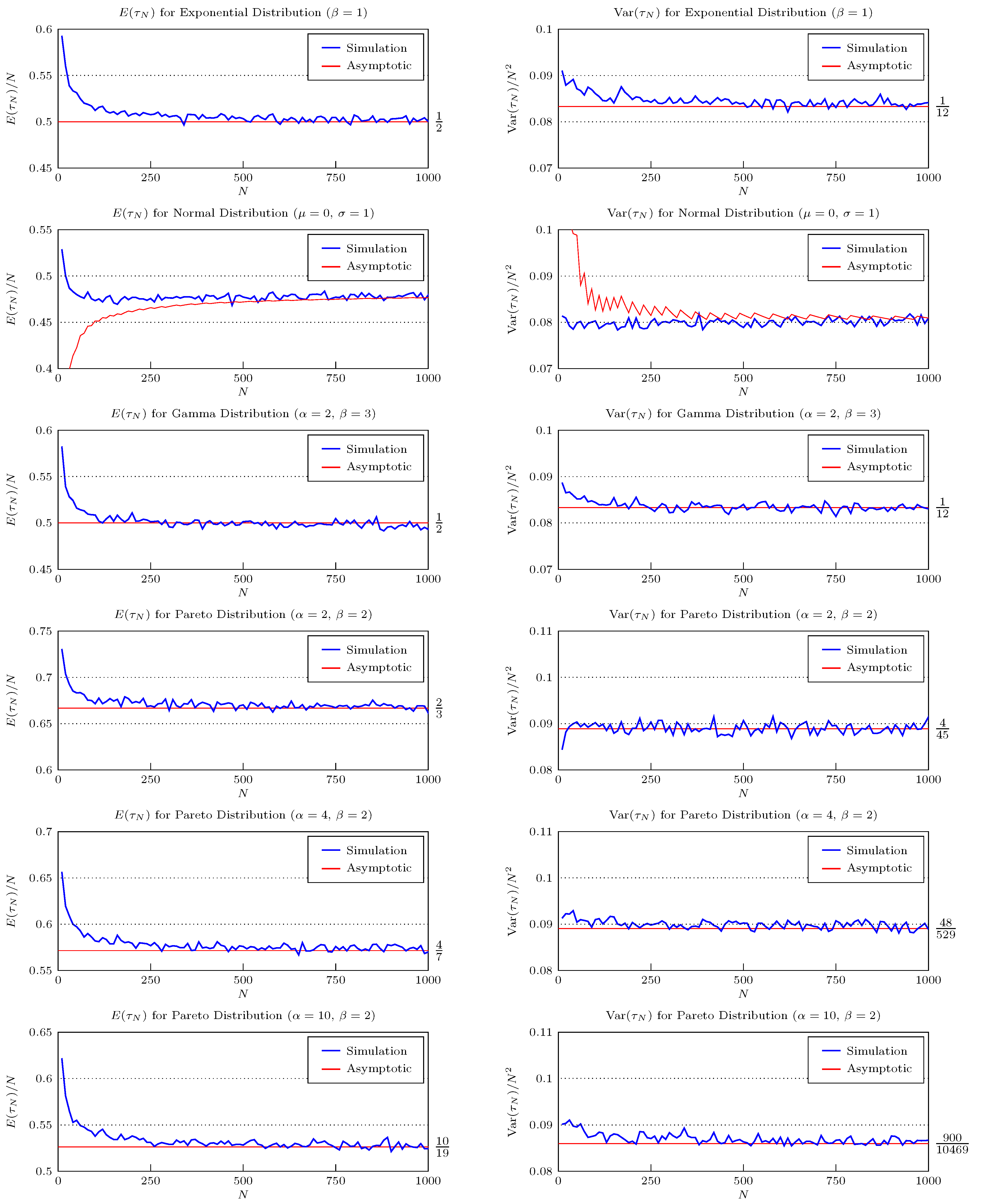
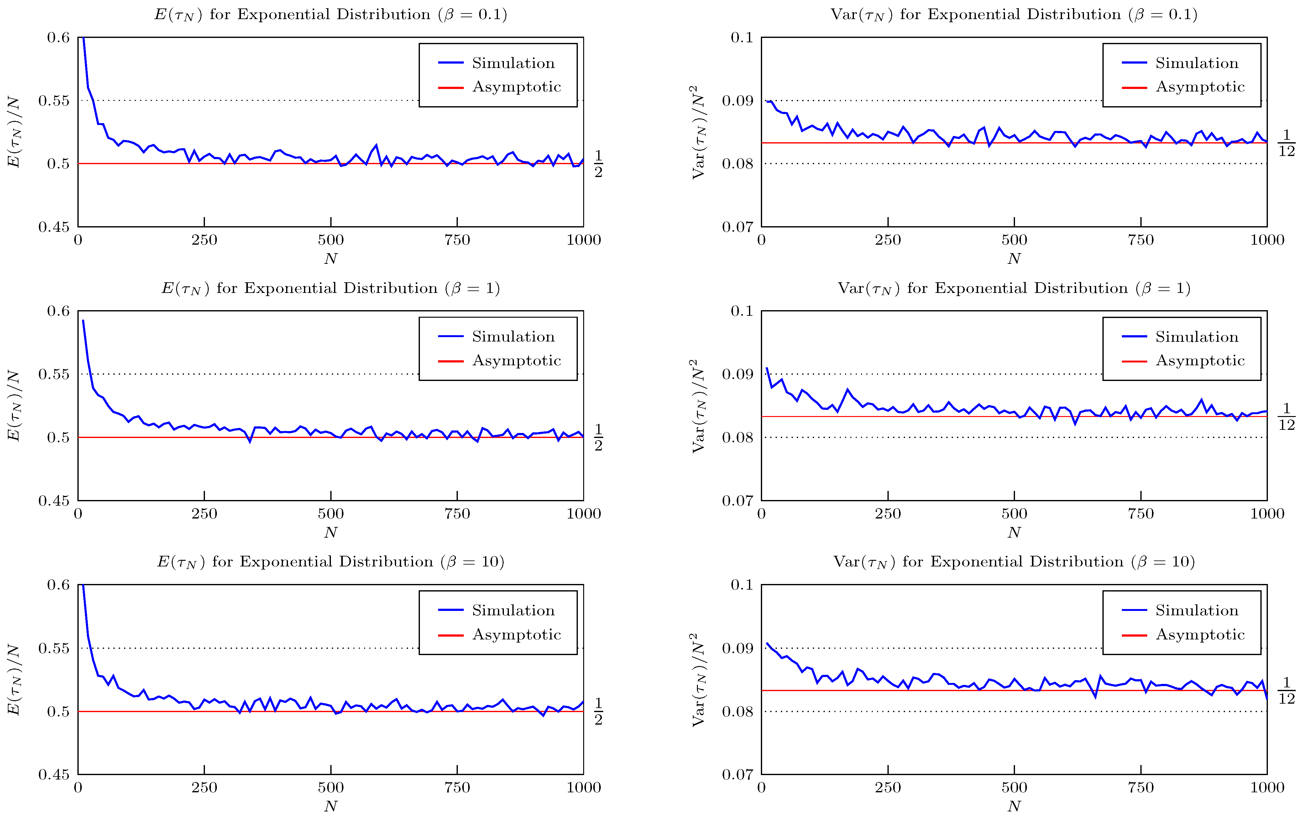
| Exponential | 1 | ||||
| Gamma | 1 | ||||
| Pareto | |||||
| Distribution | Domain | as | Var() | ||
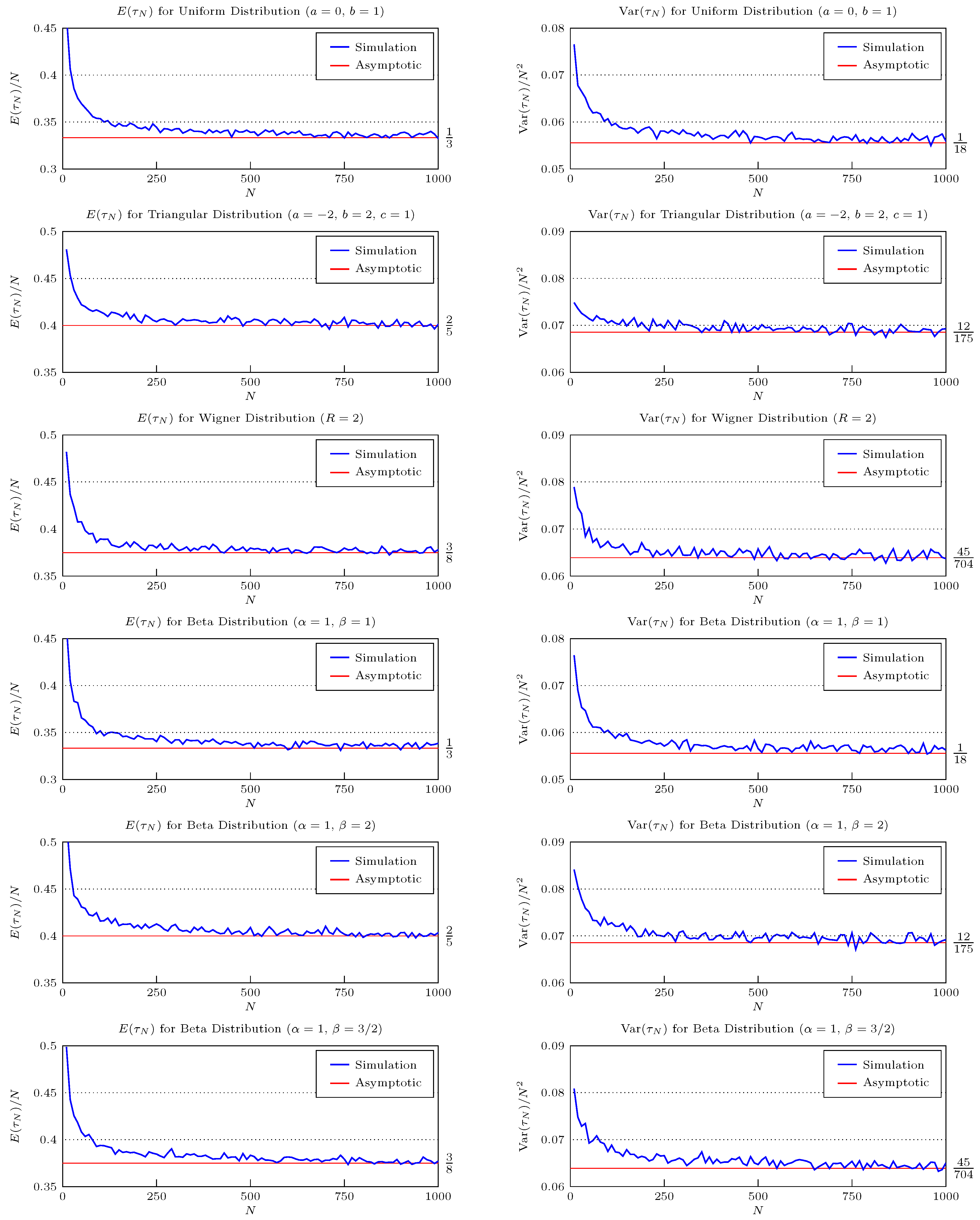
| Uniform | 2 | ||||
| Triangular | |||||
| Wigner | |||||
| Beta |
| 1.75 | 2 | 2.25 | 2.5 | 2.75 | 3 | 3.25 | 3.5 | |
| Chebyshev Bound | 0.1701 | 0.2222 | 0.2813 | 0.3472 | 0.4201 | 0.5000 | 0.5868 | 0.6806 |
| Simulated Result | 0.0103 | 0.0318 | 0.0541 | 0.0790 | 0.0977 | 0.1148 | 0.1834 | 0.2401 |
Publisher’s Note: MDPI stays neutral with regard to jurisdictional claims in published maps and institutional affiliations. |
© 2022 by the authors. Licensee MDPI, Basel, Switzerland. This article is an open access article distributed under the terms and conditions of the Creative Commons Attribution (CC BY) license (https://creativecommons.org/licenses/by/4.0/).
Share and Cite
Entwistle, H.N.; Lustri, C.J.; Sofronov, G.Y. On Asymptotics of Optimal Stopping Times. Mathematics 2022, 10, 194. https://doi.org/10.3390/math10020194
Entwistle HN, Lustri CJ, Sofronov GY. On Asymptotics of Optimal Stopping Times. Mathematics. 2022; 10(2):194. https://doi.org/10.3390/math10020194
Chicago/Turabian StyleEntwistle, Hugh N., Christopher J. Lustri, and Georgy Yu. Sofronov. 2022. "On Asymptotics of Optimal Stopping Times" Mathematics 10, no. 2: 194. https://doi.org/10.3390/math10020194
APA StyleEntwistle, H. N., Lustri, C. J., & Sofronov, G. Y. (2022). On Asymptotics of Optimal Stopping Times. Mathematics, 10(2), 194. https://doi.org/10.3390/math10020194