COVID-19 Spread Forecasting, Mathematical Methods vs. Machine Learning, Moscow Case

Abstract

To predict the spread of the new coronavirus infection COVID-19, the critical values of spread indicators have been determined for deciding on the introduction of restrictive measures using the city of Moscow as an example. A model was developed using classical methods of mathematical modeling based on exponential regression, the accuracy of the forecast was estimated, and the shortcomings of mathematical methods for predicting the spread of infection for more than two weeks. As a solution to the problem of the accuracy of long-term forecasts for more than two weeks, two models based on machine learning methods are proposed: a recurrent neural network with two layers of long short-term memory (LSTM) blocks and a 1-D convolutional neural network with a description of the choice of an optimization algorithm. The forecast accuracy of ML models was evaluated in comparison with the exponential regression model and one another using the example of data on the number of COVID-19 cases in the city of Moscow.

1. Introduction

In the context of the sanitary and epidemiological situation in Moscow associated with the spread of the new coronavirus infection COVID-19, the task of predicting the dynamics of the spread of infection and the question of when to implement quarantine measures at the regional level remains urgent. Since the start of the pandemic, the development of methods for predicting indicators characterizing the spread of coronavirus infection has remained active. The most widely used model of logistic growth [1,2,3,4] is the coplanar model, susceptible-infectious-recovered (SIR), and its various variations: susceptible-infectious-recovered-susceptible (SIRS), susceptible-exposed-infectious-recovered (SEIR), susceptible-infectious, recovered-deceased (SIRD), susceptible-infectious-recovered-vaccinated (SIRV) [5,6,7,8,9,10,11,12,13,14], and others [15,16,17,18]. However, as the complexity of the model grows, there is a concomitant increase in the number of unknown parameters, which are often difficult to estimate. Coplanar models of the type SIR, SIRS, SEIR, etc., can be used in long-term forecasting, but only for inhomogeneous isolated systems in which the law of mass action is fulfilled and good mixing of the population is observed. Real large systems cannot be considered isolated due to many factors. For example, Moscow and the Moscow agglomeration are characterized by commuting (more than 2 million people per day), including migration from neighboring regions (Tula, Vladimir, and Kaluga regions), and a large number of departures and arrivals per day (more than 100 thousand people per day). In addition, the listed methods allow simulating only one wave of a pandemic and do not take into account the possibility that during one wave, there may be many “peaks” of the incidence. At the same time, machine learning methods are more versatile since a trained neural network is capable of making predictions on a variety of systems, given the possibility of multimodal patterns in the past.

Models using the discrete logistic Feigenbaum equation also show good results [19,20]. However, the vast majority of mathematical models cannot predict with acceptable accuracy for more than two weeks. This is due to the same fact: real systems, such as cities, separate regions, or countries, are open and heterogeneous. As a result, many new sources of infection accidentally appear in systems, launching new chains of transmission of coronavirus from infected to susceptible. It should also be noted that statistical data from official sources contains large errors, ranging from 15% to 75% [19,21].

It is also worth noting the existence of several synthetic models, including the combination of methods of mathematical epidemiological modeling and machine learning methods, for example, the combination of neural networks and ensembles of neural networks with modified spatio-temporal disease models [22,23,24]. Such models show very accurate results in predicting the spread of new coronavirus infection, making it possible to compensate for the shortcomings of each method separately.

This article examines the time series of the number of cases of new coronavirus infection and the number of hospitalizations in one-day increments. By the type of behavior, they are classified as a non-stationary time series since the statistical properties of the series change over time (since different “waves” of incidence have different characteristics) and as a regular time series (since data are received at regular intervals—1 day). There are many classical methods for analyzing and forecasting time series, for example, various types of regression analysis, e.g., linear, polynomial, exponential, ridge regression, least absolute shrinkage, and selection operator (LASSO) regression. For predicting time series, singular spectrum analysis (SSA), interpolation by matching pursuit (MIMAP), least-squares spectral analysis (LSSA), antileakage least-squares spectral nalysis (ALLSSA) [25], in addition to models of Fourier series methods, autoregressive models of the form autoregressive integrated moving average (ARIMA), trend and seasonal components (TBATS), and locally estimated scatterplot smoothing (LESS) models [26] are employed. Among the machine learning methods for predicting the spread of COVID-19, fairly accurate results are obtained by methods based on support vector machine (SVM), wavelet neural network (WNN), and bidirectional long short-term memory (Bi-LSTM) [26,27].

At the first stage of the study, modeling was carried out using an exponential regression equation suitable for describing the onset of an epidemic or the beginning of the next “wave” based on the statistics of cases of infection and hospitalization in the city of Moscow. This method has shown good results in terms of prediction accuracy for a period of up to two weeks. For the second stage of the study, prediction methods based on machine learning algorithms were used on a sample of cases of COVID-19 infection from 21 systems, including data from the city of Moscow. The study built neural networks based on LSTM and convolutional neural network (CNN) architectures to predict the spread of coronavirus infection over a longer period of 48 days. This paper presents the results of predicting the number of cases of infection with a new coronavirus infection in the city of Moscow.

The structure of the article is as follows. Section 2 describes how to find critical parameters for making a decision regarding the introduction of restrictive measures, constructing an exponential regression model and forecasting based on it, the principles of sampling a dataset for training a neural network, as well as the architecture of the proposed neural networks. Section 3 describes the results of the training and validation of the proposed sample-based neural network architectures, comparing the prediction accuracy of classical mathematical methods and machine learning methods using the example of the obtained predictions, and comparing the prediction accuracy of the proposed neural network architectures. Section 4 summarizes the study’s findings on the use of mathematical methods for modeling the long term incidence of COVID-19 infections and machine learning methods. Section 5 formulates the main conclusion of this work.

2. Materials and Methods

2.1. Determination of Predicted Parameters

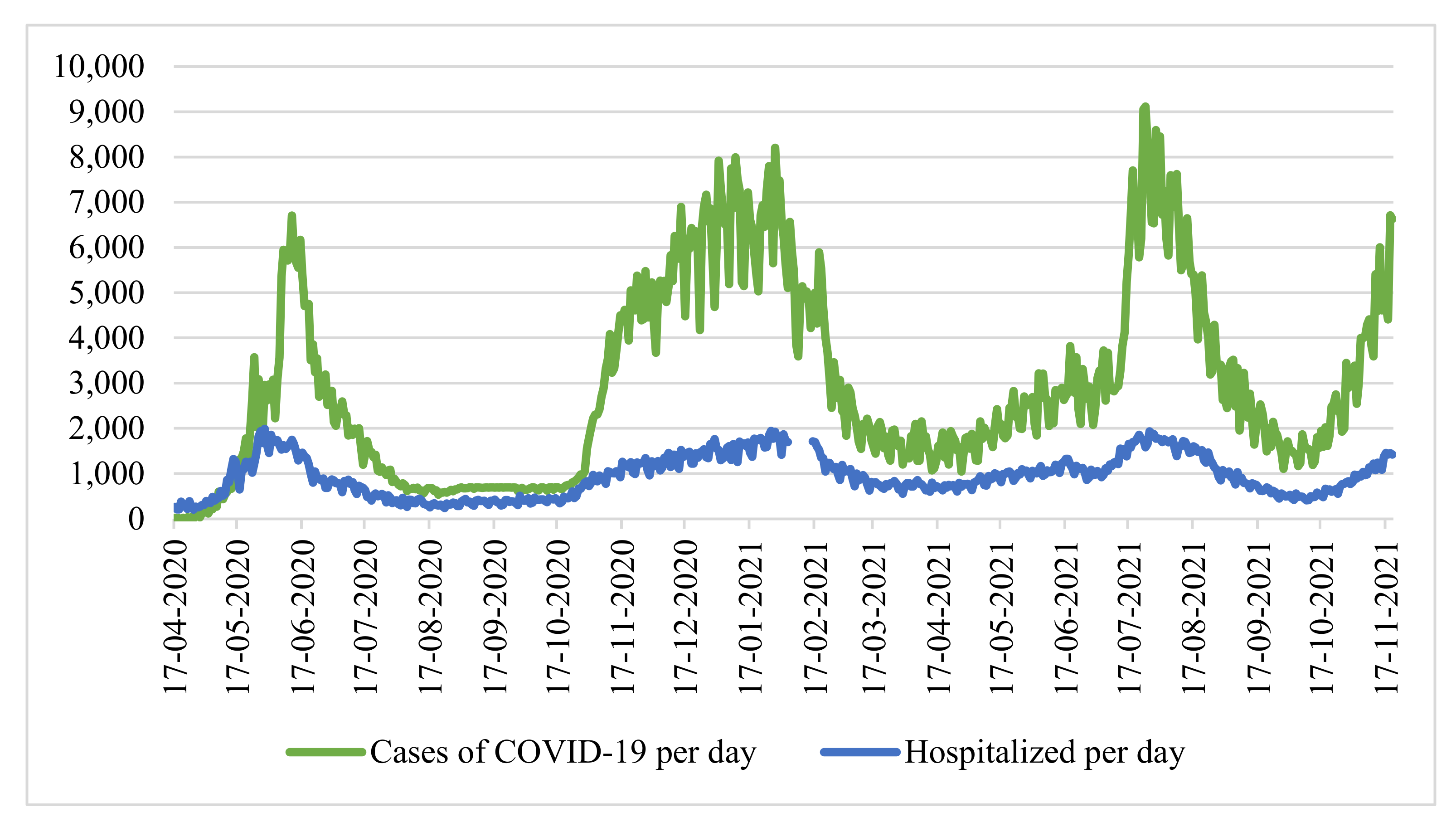
To begin the study, it is necessary to identify the possible factors influencing the adoption of measures. As for Moscow, the decrees of the mayor of Moscow do not indicate specific indicators used to make decisions on restrictions on the movement of the population [28,29]. However, the features of COVID-19 are already well known, which is characterized by high contagiousness, a long incubation period, and a rather high probability of serious complications requiring inpatient treatment. All of these factors combine to quickly overwhelm the healthcare system. Therefore, it is natural to take the number of infections per day and the number of hospitalized patients with COVID-19 per day as the baseline indicators of the study. The first parameter reflects the spread of new coronavirus infection, and the second parameter (the number of hospitalized) reflects the load on the bed fund and the healthcare system as a whole. The achievement of a certain critical level by these parameters becomes a significant reason for deciding to impose restrictions.

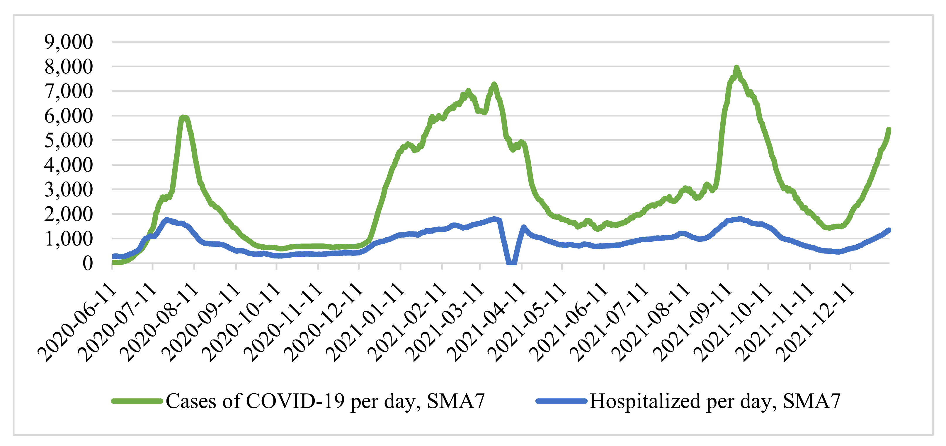
We conducted a study using the example of Moscow. We considered the time series of cases of coronavirus infection and the number of hospitalized patients in the city of Moscow from 12 March 2020 to 15 October 2021 (Figure 1) [30]. At the same time, there are no data for the period from 31 December 2020 to 10 January 2021, since the Moscow operational headquarters did not publish statistics on the number of hospitalized individuals with a new coronavirus infection during this period.

Denote the number of cases of COVID-19 infection per day by the function f(t), and the number of hospitalized by the function φ(t), where t is a step in time (day). To check whether it is necessary to simultaneously use both indicators, we calculated the Pearson correlation coefficient:

$${\mathrm{r}}_{F\mathsf{\Phi }}=\frac{cov\left(F,\mathsf{\Phi }\right)}{{\sigma }_F{\sigma }_{\mathsf{\Phi }}}=\frac{{{\displaystyle \sum }}_{i=1}^n\left[\left(F_i-\overline{F}\right)\left({\mathsf{\Phi }}_i-\overline{\mathsf{\Phi }}\right)\right]}{\sqrt{{{\displaystyle \sum }}_{i=1}^n{\left(F_i-\overline{F}\right)}^2{{\displaystyle \sum }}_{i=1}^n{\left({\mathsf{\Phi }}_i-\overline{\mathsf{\Phi }}\right)}^2}},$$

(1)

where: $F=f\left(t\right)$—number of cases per day $t$, $\mathsf{\Phi }=\phi \left(t\right)$—number of hospitalized per day $t$, $\overline{F}$ and $\overline{\mathsf{\Phi }}$—the arithmetic mean of the sample. To eliminate the difference in sample size associated with the lack of data on hospitalizations from 31 December 2020 to 10 December 2020, the corresponding values for the number of infections were removed.

The correlation coefficient for the entire sample size is 0.866735, which characterizes the level of linear relationship as high. However, considering the periods of “waves”, we note that the number of hospitalized people grows in proportion to the number of infected individuals. Therefore, in the period from 1 October 2020 to 31 December 2020 (main stage “second” wave of coronavirus), the coefficient $r_{F\mathsf{\Phi }}$ was only 0.627 (weak—moderate on the scale of E.P. Golubkov), and during the period of active growth of the third wave (from 9 June 2021 to 22 July 2021), the coefficient was 0.636 (moderate).

This discrepancy is explained by the following: in periods between waves of morbidity, the healthcare system can hospitalize a larger number of patients (including those with mild and moderate disease), and during a period of active growth, the healthcare system is forced to refuse hospitalization for patients with mild and moderately mild disease due to insufficient bed capacity, hospitalizing only moderately and seriously ill patients. Due to this fact, during periods of “waves”, the correlation between the number of hospitalized and sick people is noticeably weak, as a result of which it is necessary to consider both factors as influencing the decision to introduce measures aimed at improving the sanitary and epidemiological situation.

Since the time series above (Figure 1) is characterized by strong daily changes, we applied a seven-day moving average, simple moving average (SMA7):

$$SM{A}_t=\frac{1}{7}{\displaystyle \sum }_{i=0}^6{p}_{t-i},$$

(2)

where: $p_{t-i}$ is the number of cases of hospitalizations at the point $t-i$. As a result, we obtained a smoothed time series (Figure 2).

We determined the “critical” values of the parameters based on the dates of the introduction of measures aimed at stabilizing the epidemiological situation: 13 November 2020 to 13 June 2021. It is known that the duration of the disease from the moment of onset of symptoms in the case of moderate to severe averages 28 days [31]. Taking this into account, we determined the cumulative number of patients in the period up to the moment $t_1$ = 13.11.2020 at $F_1$, in the period before $t_2$ = 13.06.2021 at $F_2$:

$$F_1={\displaystyle \sum }_{i=0}^{27}f\left(t_1-i\right)=143596 \left(person\right)$$

(3)

$$F_2={\displaystyle \sum }_{i=0}^{27}f\left(t_2-i\right)=92705 \left(person\right)$$

(4)

Similarly, we determines the cumulative number of hospitalized individuals in the period up to the moments $t_1$—for ${\mathsf{\Phi }}_1$ and $t_2$—for${\mathsf{\Phi }}_2$:

$${\mathsf{\Phi }}_1={\displaystyle \sum }_{i=0}^{27}\phi \left(t_1-i\right)=34848\left(person\right)$$

(5)

$${\mathsf{\Phi }}_2={\displaystyle \sum }_{i=0}^{27}\phi \left(t_2-i\right)=32610\left(person\right)$$

(6)

At the time of making decisions on the introduction of new restrictive measures, the indicators of the cumulative number of hospitalized ${\mathsf{\Phi }}_1$ and ${\mathsf{\Phi }}_2$ are approximately similar. However, the difference between $F_1$ and $F_2$ is significant. From the smoothed time series of the number of cases (Figure 2), it can be seen that the growth of incidence rates in the first case is more uniform than in the second, which was more “explosive”.

For a more detailed analysis, we used the Rt Coronavirus Spread Index, also known as the effective reproductive number. This indicator reflected the rate of growth of new cases of new coronavirus infection, calculated using the “4 by 4” method:

$$Rt=\frac{{{\displaystyle \sum }}_{i=0}^{3}f\left(i\right)}{{{\displaystyle \sum }}_{i=4}^{7}f\left(i\right)}=\frac{F_0+F_1+F_2+F_3}{F_4+F_5+F_6+F_7},$$

(7)

where $F_0$ is the current day. In other words, the number of people infected in the last 4 days (including the current one) is divided by the number of people infected in the previous 4 days.

This indicator, used by Rospotrebnadzor as a metric for deciding whether to soften or strengthen restrictive measures, shows how many people manage to infect one infected person before they are isolated. If Rt < 1, Rospotrebnadzor recommends starting to mitigate restrictive measures. The calculation according to the “4 by 4” formula makes it possible to smooth out daily fluctuations in the number of detected cases of COVID-19 infection, occurring due to the different number of tests taken and processed to detect a new coronavirus infection.

The spread of coronavirus was also considered in conjunction with the baseline reproduction rate R₀ (baseline reproductive number). R₀ is the average number of people who are infected by one carrier in a naive population, that is, a population whose citizens do not have immunity to this disease at all and do not take any measures to protect themselves from it. We can say that at the beginning of the epidemic, Rt coincided with R₀. The baseline reproduction rate cannot be measured directly, and its value depends on the chosen model of the infection mechanism and, at the same time, remains constant. Several studies also indicate that the basic reproductive number R₀ does not take into account the presence of “super-spreaders” and individual differences in infectivity and is often highly distorted [32,33,34]. Therefore, for research purposes, the R₀ level is not of interest.

We considered the dynamics of the index in the first and second moments during the three days before and after the introduction of measures to reduce the incidence (

Table 1. Dynamics of the Rt index before and before the introduction of restrictions.

Date	Cases of COVID-19 per Day	Rt	Date	Cases of COVID-19 per Day	Rt
10 November 2020	6897	1.176	10 June 2021	4124	1.237
11 November 2020	5902	1.084	11 June 2021	5245	1.427
12 November 2020	4477	0.994	12 June 2021	5853	1.598
13 November 2020	5997	1.008	13 June 2021	6701	1.697
14 November 2020	5974	0.904	14 June 2021	7704	1.803
15 November 2020	6427	0.938	15 June 2021	6590	1.632
16 November 2020	6271	1.071	16 June 2021	6805	1.460

).

With the introduction of restrictive measures in November 2020, the average value of the index was 1.02. When the restrictive measures were introduced in June 2021, the average value of the index was 1.54. Moreover, in June 2021, there was a significant increase in the number of cases of the disease, which had an additional impact on the decision to introduce restrictive measures.

2.2. Forecasting Based on the Exponential Model

For further analysis and prognosis, it is required to approximate the values of the number of cases of the disease and the number of hospitalizations. Note that during the period of increasing incidence, the growth is exponential. Thus, the function of the number of cases of the disease can be represented as:

$$f\left(t\right)=\beta \times \exp \left(\alpha t\right),$$

(8)

where $\alpha$, $\beta$—some ratios. Whence, after taking the logarithm, we obtain:

$$\ln \left(f\left(t\right)\right)=\ln (\beta )+\alpha \times t$$

(9)

Suppose $Y=\ln \left(f\left(t\right)\right),B=\ln \left(\beta \right),A=\alpha$, then the function can be represented as:

$$Y=A\times t+B$$

(10)

In this case, the problem is reduced to estimating the parameters of the paired linear regression model using the least-squares method:

$$F={\displaystyle \sum }_{i=1}^n{\left[Y_i-\left(A\times t_i+B\right)\right]}^2\to min,$$

(11)

Then the estimates of the coefficients can be found by the formula:

$$A=\frac{n{{\displaystyle \sum }}_{i=1}^n\left(t_i\times Y_i\right)-{{\displaystyle \sum }}_{i=1}^n{t}_i{{\displaystyle \sum }}_{i=1}^n{Y}_i}{n{{\displaystyle \sum }}_{i=1}^n{t}_i^2-{\left({{\displaystyle \sum }}_{i=1}^n{t}_i\right)}^2}$$

(12)

$$B=\frac{{{\displaystyle \sum }}_{i=1}^n{Y}_i-A{{\displaystyle \sum }}_{i=1}^n{t}_i}{n}$$

(13)

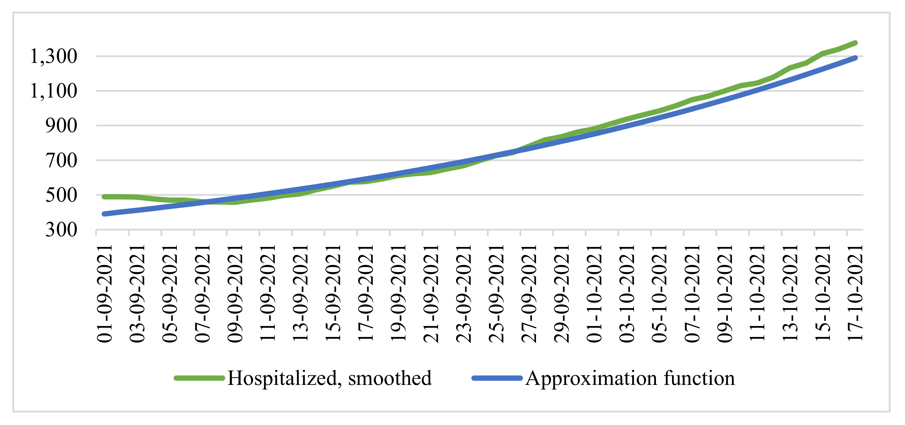
Approximating the data on the smoothed time series from 1 September 2021 to 16 October 2021, we obtain:

$$f\left(t\right)=1151.9\times e^{0.033t}$$

(14)

We compared the data of the time series of smoothed values of infection cases and the resulting function (Figure 3).

In this case, the coefficient of determination $R^2$ was 0.9918, which characterizes the model on the segment as satisfactory. Note that forecasting based on the exponential model allows us to very accurately simulate the initial growth period occurring in real-time.

In Figure 3, it can be seen that $f\left(t\right)$ is lagging from the real number of cases per day, but it is the lag of the function $f\left(t\right)$ « from the actual current indicators that will increase the forecast accuracy over a short time interval since the values of $f\left(t\right)$ will be higher than the increase in morbidity in the long run. Since, at the moment, the average value of the $Rt$ index in the period over the past 7 days is 1.1, it is logical to assume that the critical value of the number of cases of the disease, further denoted as $F_3,$ is more likely to impact the value of $F_1$ (143,496 people) than the value of $F_2$, since in June, there was a rapid increase in cases, which is currently not observed. Similarly, we assumed that the critical value of the number of hospitalized individuals, hereinafter denoted as ${\mathsf{\Phi }}_3$, was more likely to impact the value of ${\mathsf{\Phi }}_1$ (34,848 people).

We apply the same approximation method for the values of the function of the number of hospitalized patients $\phi \left(t\right)$, as a result of which:

$$\phi \left(t\right)=390.39\times e^{0.026t}$$

(15)

We compared the data of the time series of smoothed values of the number of hospitalized people and the resulting function (Figure 4).

In this case, the coefficient of determination $R^2$ was 0.9869, which also characterized the model on the segment as quite good.

For forecasting, we defined the confidence interval estimates of the coefficients $a_1=\alpha ,a_0=\ln \left(\beta \right)$ for the period from 1 September 2021 to 17 October 2021 from the exponential model of the approximation functions $f\left(t\right)$ and $\phi \left(t\right)$, corresponding to the reliability of 95% according to the formulas:

$${\xi }_{0.05;45}\frac{s_{ELR}}{\sqrt{{{\displaystyle \sum }}_{i=1}^{47}{\left(t_i-\overline{t}\right)}^2}}<a_1<{\widehat{a}}_1+{\xi }_{0.05;45}\frac{s_{ELR}}{\sqrt{{{\displaystyle \sum }}_{i=1}^{47}{\left(t_i-\overline{t}\right)}^2}}$$

(16)

$${\widehat{a}}_0-{\xi }_{0.05;45}\frac{s_{ELR}\sqrt{{{\displaystyle \sum }}_{i=1}^{47}{t}_i^2}}{\sqrt{47{{\displaystyle \sum }}_{i=1}^{47}{\left(t_i-\overline{t}\right)}^2}}<a_0<{\widehat{a}}_0+{\xi }_{0.05;45}\frac{s_{ELR}\sqrt{{{\displaystyle \sum }}_{i=1}^{47}{t}_i^2}}{\sqrt{47{{\displaystyle \sum }}_{i=1}^{47}{\left(t_i-\overline{t}\right)}^2}}$$

(17)

where ${\xi }_{0.05;45}$ is a two-sided critical point of the student distribution with 45 degrees of freedom, corresponding to a probability of 0.05, $s_{ELR}$ is an unbiased estimate of the standard deviation of the regression equation.

We denoted the values of the point estimates of the coefficients $a_1$ and $a_0$ for the base forecast, the positive forecast, the lower limit of the confidence interval, the negative, and the upper limit confidence interval (

Table 2. Coefficients of paired linear regression for predictions.

	Index	$\mathit{\alpha } \mathit{f}\left(\mathit{t}\right)$	$\mathit{\beta } \mathit{f}\left(\mathit{t}\right)$	$\mathit{\alpha } \mathit{\phi }\left(\mathit{t}\right)$	$\mathit{\beta } \mathit{\phi }\left(\mathit{t}\right)$
Forecast
Positive		0.03133	1151.85544	0.02451	390.32033
Base		0.033	1151.9	0.026	390.36
Negative		0.03466	1151.94455	0.02748	390.39966

).

Based on the factors listed above, we considered the forecast of a seven-day moving average of cases of COVID-19 infection from 17 October 2021 to 10 November 2021 based on the values of the function $f\left(t\right)$ (Figure 5).

In this period, we considered the cumulative number of infections over the last 28 days and defined it as the “critical” value $F_3$ = 150,000 people:

• With the baseline forecast, the first date of reaching the critical value: 29 October 2021.
• In case of a negative forecast, the first date of reaching the critical value: 28 October 2021.
• With a positive forecast, the first date of reaching the critical value: 31 October 2021.

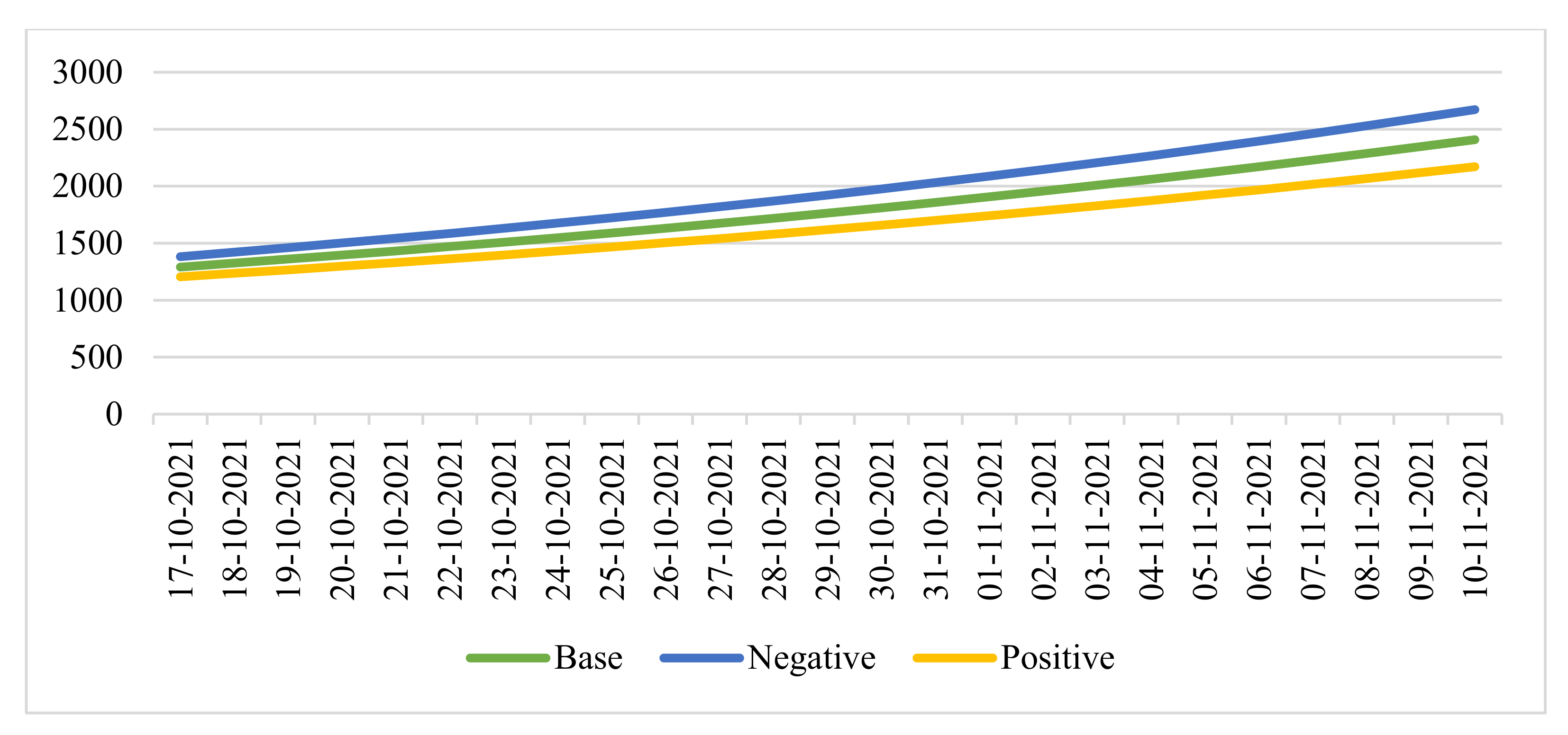
Similarly, we considered the forecast of a seven-day moving average number of hospitalizations based on the values of the function $\phi \left(t\right)$ for the same period (Figure 6).

In this period, we considered the cumulative number of hospitalizations for the last 28 days and defined it as the “critical” value ${\mathsf{\Phi }}_3$ = 36,000 people:

• With the baseline forecast, the first date of reaching the critical value: 29 October 2021.
• In case of a negative forecast, the first date of reaching the critical value: 27 October 2021.
• With a positive forecast, the first date of reaching the critical value: 30 October 2021.

Thus, based on the forecasts made, it is most likely that measures aimed at stabilizing the epidemiological situation will be taken in the period from 27 October to 31 October.

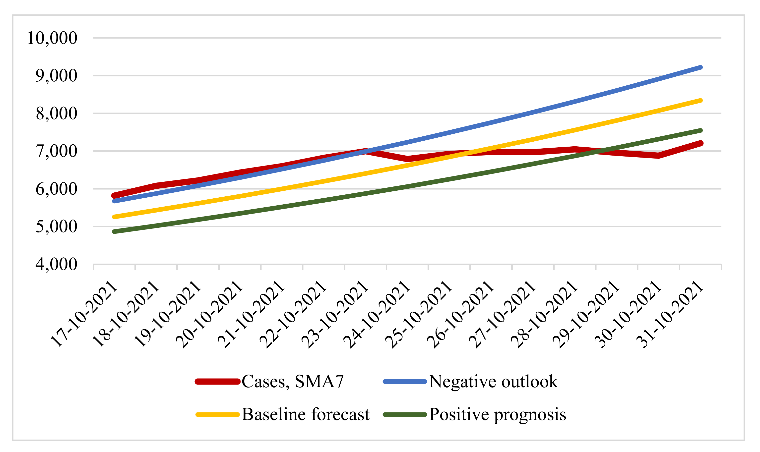
At the time of 30 October 2021, the constructed forecast was confirmed. By the decree of the mayor of Moscow, restrictions were introduced on 28 October (negative scenario according to the forecast). We then considered the seven-day rolling COVID-19 case and forecast options for the period from 17 October 2021 to 31 October 2021 (Figure 7).

We evaluated the forecast accuracy for 15 days (from 17 October 2021 to 31 October 2021) of three scenarios with real data on the number of smoothed cases of COVID-19 infection using two metrics: root mean square error (RMSE) and mean absolute percentage error (MAPE) (

Table 3. Estimates of various exponential regression predictions.

Forecast	RMSE	MAPE, %
Negative	994.942	10.171
Base	655.951	8.596
Positive	802.835	10.937

).

The table values concerning a baseline forecast with MAPE 8.596% and RMSE 655.951 showed more accurate forecast results. It can be seen that, until 23 October, the situation developed according to a negative forecast, and the introduction of restrictive measures was announced on 21 October. At the same time, it was reported that the situation was developing according to a negative forecast. However, from 24 October, the real number of cases of infection deviated from the predicted values. Here, the disadvantages of using exponential regression models for the long term are fully manifested: the number of infection cases has a “wavy” appearance, which the exponential model cannot display, as a result of which it becomes necessary to use other forecasting methods.

2.3. Determination of the Dataset and Neural Network Architectures

For further research, we turned to machine learning methods. In this case, the task of forecasting time series belongs to the supervised learning class. To form the sample, the data on the number of cases of COVID-19 infection were used from 20 countries: Austria, Belgium, Great Britain, Hungary, Germany, Israel, Iran, Spain, Italy, Canada, the Netherlands, Poland, Russia, Romania, Serbia, USA, France, Czech Republic, Switzerland, Japan, and data from the city of Moscow in the period from 18 March 2020 to 3 December 2021 [28,35,36]. These countries were selected according to two criteria: a population of more than 8 million people and a developed healthcare system. Together, these criteria made it possible to obtain sufficiently accurate and objective data on the number of cases of coronavirus infection.

To reduce the influence of daily fluctuations, a seven-day simple moving average (SMA7) was applied to the entire sample size. For the adequate operation of the neural network to all the values of these systems from the dataset separately, we applied the normalization function $f : ℝ\to \left[0,1\right]$:

$$f\left(x\right)=\frac{x-x_{min}}{x_{max}-x_{min}},$$

(18)

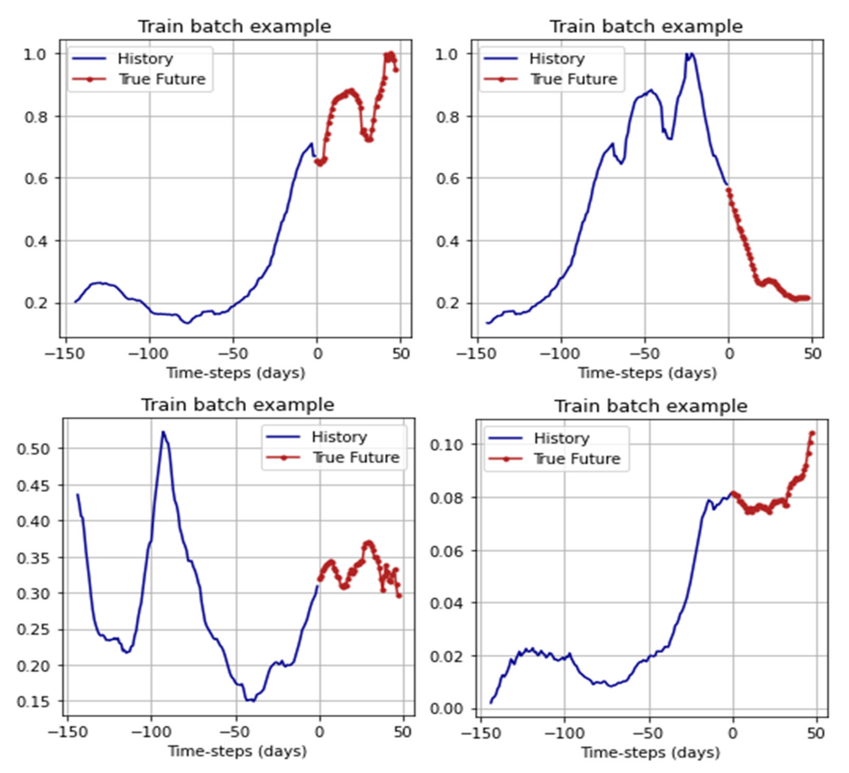
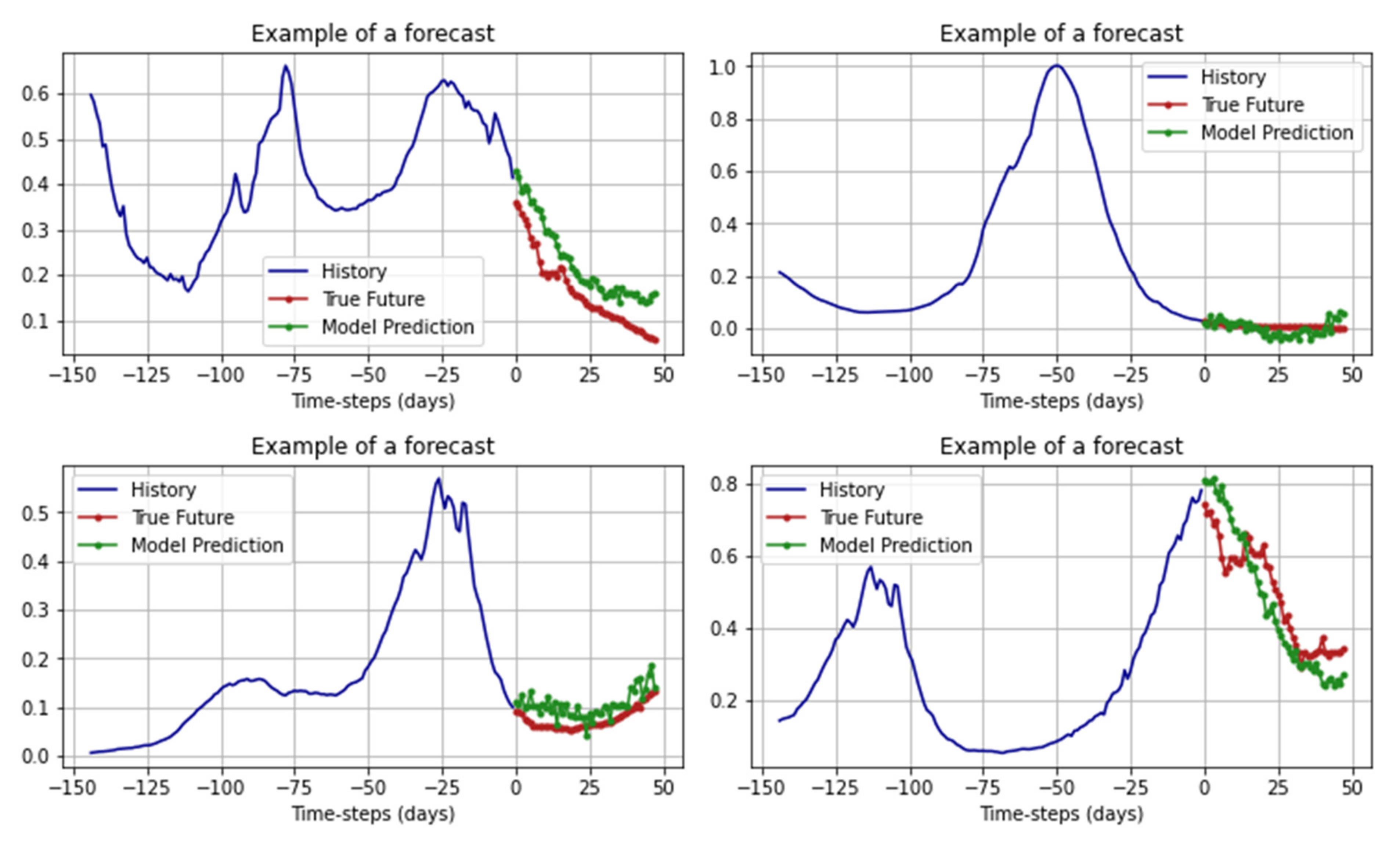
where $x$ is SMA7 infections per day, $x_{max}$ and $x_{min}$ are the the maximum and a minimum number of cases of COVID-19 infection in the system, respectively. To normalize the data, the MinMaxScaler class from the scikit-learn library was used. Thus, all values were in the range from 0 to 1 in the corresponding scale. Figure 8 show examples of data from several systems.

The dataset length was 626 values, of which 67% (419 values from each system) were intended for the training sample, and the remaining 33% (207 values from each system) were intended for the validation sample. The entire amount of data was 13,146 values.

For training, the networks received batches: 144 days before the forecast period as data based on which the forecast was made, and 48 days for the forecast. From the original dataset, 5775 batches were generated for training and 315 batches for validation. For efficiency, the batchhes were shuffled using the shuffle method from the TensorFlow framework. Examples of the batches are shown in Figure 9.

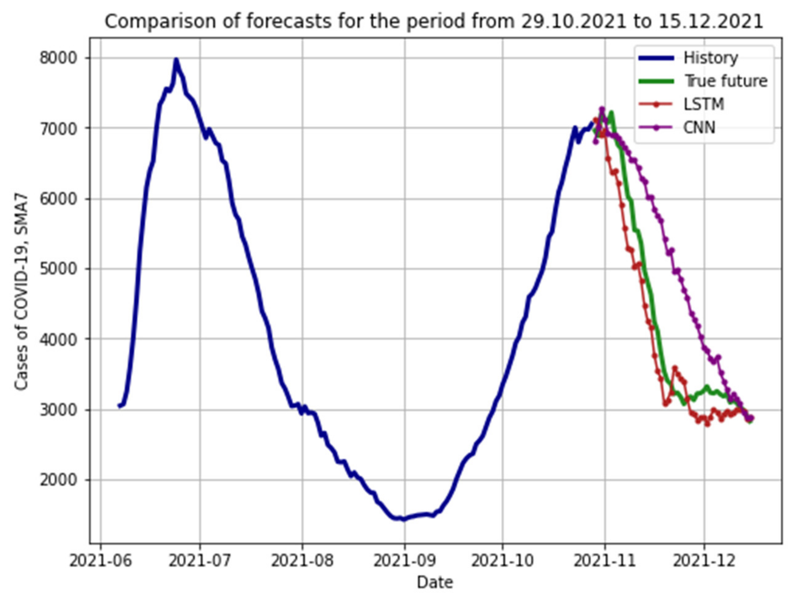
To predict the time series of the number of cases of COVID-19 infection, we used two types of neural networks: long short-time memory (LSTM) and a convolutional neural network. We considered in more detail the architecture of the LSTM recurrent neural network, which is one of the most suitable ML-models for forecasting time series. The main advantage of this architecture is its good adaptability to learning and forecasting in a situation where key events (in our case, the “waves” of the coronavirus) are separated by indefinite time intervals, and their time boundaries are different. The architecture of the LSTM RNN network can be represented as:

$$\{\begin{array}{c}{f}_t={\sigma }_g\left(W_f\times \left[x_t,h_{t-1}\right]+b_f\right)\\ i_t={\sigma }_g\left(W_i\times \left[x_t,h_{t-1}\right]+b_i\right)\\ \widetilde{C_t}={\sigma }_g\left(W_C\times \left[x_t,h_{t-1}\right]+b_c\right)\\ C_t=f_t\times C_{t-1}+i_t\times \widetilde{C_t}\\ o_t={\sigma }_g\left(W_o\times \left[x_t,h_{t-1}\right]+b_0\right)\\ h_t=o_t\times {\sigma }_g\left(c_t\right)\end{array}$$

(19)

where, $x_t$is the input vector, $f_t$ is the loss layer, $i_t$is the input gate layer, $\widetilde{C_t} \mathrm{and} C_t$ are the state vectors, $o_t$ is the output gate layer, $h_t$is the target (output) vector, $W, b$ are the vectors of parameters (weights) [37].

In this case, the neural network was trained to predict 48 days based on data from the previous 144 days. Thus, the input vector $x_t$is:

$$x_t=\left(\begin{array}{c}{a}_{t-1}\\ a_{t-2}\\ ⋮\\ a_{t-144}\end{array}\right)$$

(20)

where, $a_i$ is the number of cases of COVID-19, SMA7. Since the number of neurons in the output layer is determined by the number of forecast days, this value is 48 pieces. LSTM RNNs work with sequences and require data of the following form as input: [observations, time interval, number of signs]. In our case, the time interval was equal to one (the step is equal to one day). Therefore, we took a closer look at the two hidden layers.

The first hidden layer consisted of 144 LSTM blocks with the activation function in the form of a hyperbolic tangent. The second hidden layer consisted of 48 LSTM blocks and used the rectified linear unit (ReLU) as the activation function. Between the two hidden layers was dropout with a factor of 0.3 to combat overfitting. The total number of parameters for training in this network model was 123,504. In more detail, the proposed architecture with the names of layers from the TensorFlow framework can be seen in

Table 4. The architecture of the LSTM RNN.

Layer’s Type	Quantity	Output Shape	Activation	Params
LSTM	144	(None; 144; 144)	Tanh	84,096
Dropout	0.3
LSTM	48	(None, 48)	ReLU	37,056
Dense	48	(None, 48)	None	2352
Total parameters:	123,504

.

We also took a closer look at the architecture of the second neural network for predicting cases of COVID-19 infection—the convolutional neural network. The principle of operation of this network is to alternate convolutional layers and subsampling layers (pooling layers).

In this model, the first convolution layer formed 64 output filters in convolution; the size of the one-dimensional convolution window was two. Then there was a downsampling layer with a window size equal to the convolution window size, that is, 2, and a flattened layer. This was followed by two fully connected layers of 50 neurons and 48 output neurons. The total number of trained parameters was 229890. In more detail, the network architecture with the names of the layers from the TensorFlow framework is given in

Table 5. The architecture of the CNN.

Layer’s Type	Quantity	Output Shape	Activation	Params
Conv1D	-	(None; 143; 64)	ReLU	192
MaxPooling1D	-	(None; 71; 64)	-	0
Flatten	-	(None; 4544)	-	0
Dense	50	(None; 50)	ReLU	227,250
Dense	48	(None; 48)	None	2448
Total params:	229,890

.

The classical indicator was used as the loss functions for training both networks of mean squared error ($MSE)$:

$$MSE=\frac{1}{m}{\displaystyle \sum }_{i=1}^m{\left(y_i-\widehat{y_i}\right)}^2,$$

(21)

where, $y_i$ is the true meaning, $\widehat{y_i}$ is the estimated value.

We considered in more detail the choice of the optimization algorithm. There are many different methods, but the most preferable is the method of adaptive estimation of the moment, Adam, due to the combination of the accumulation of the motion of the gradient of the loss function and the relatively weak update of weights for typical features.

We considered its work in more detail. First, the algorithm updates the exponential moving averages of the gradient $m_t$, which is the estimate of the 1st moment (mean):

$$m_t={\beta }_1{m}_{t-1}+\left(1+{\beta }_1\right){\nabla }_W{f}_t\left(W\right)$$

(22)

where ${\beta }_1$ is a hyperparameter that controls the exponential decay rates of the sliding, while $0\ll {\beta }_1<1$. ${\nabla }_W{f}_t\left(W\right)$ is the objective function gradient (vector of partial derivatives $f_t)$. On the recommendation of the authors for machine learning problems ${\beta }_1=0.9$ [38]. To estimate the frequency of the gradient change, the average non-centered variance is used) $v_t$:

$$v_t={\beta }_2{m}_{t-1}+\left(1+{\beta }_2\right){\left[{\nabla }_W{f}_t\left(W\right)\right]}^2$$

(23)

where, ${\beta }_2$—similar ${\beta }_1$ the hyperparameter that controls the exponential decay rates of the sliding, and is taken as 0.999 as the most appropriate value for machine learning problems [39,40]. However, these slides are initialized as vectors close to zero (and the values will accumulate for a long time). To correct this problem, the first and second moments $m_t$ and $v_t$ are calculated, corrected for displacement:

$${\widehat{m}}_t=\frac{m_t}{1-{\beta }_1^t},{\widehat{v}}_t=\frac{v_t}{1-{\beta }_2^t}$$

(24)

As a result, the weights are updated according to the rule:

$$W_{t+1}=W_t-\frac{\eta }{\sqrt{{\widehat{v}}_t+\epsilon }}{\widehat{m}}_t$$

(25)

where, $\eta$—learning rate, $\epsilon ={10}^{-8}—$smoothing parameter.

3. Results

3.1. Training and Validation of Neural Network Models

The implementation of the neural network was carried out in the Python programming language in a Jupyter Notebook development environment using the open TensorFlow machine learning framework from Google as a basis (mainly a Keras add-on) with the involvement of the matplotlib libraries (for drawing graphs), scikit-learns (for normalization and network validation), and Pandas (for data structuring).

For LSTM RNN training, we determined an epoch size of 100 steps with 64 batches processing at each step and determined the number of epochs to be 24. We also considered the dynamics of the loss function on the training and test samples (Figure 10).

To validate the trained neural network, we used the mean absolute percentage error (MAPE):

$$MAPE\left(y,\widehat{y}\right)=\frac{100}{n}{\displaystyle \sum }_{i=0}^{n-1}\frac{\left|y_i-{\widehat{y}}_i\right|}{\left|y_i\right|}$$

(26)

where, $n$ is the sample size, $y_i\mathrm{and}{\widehat{y}}_i$ are the true and predicted value for the day $i$. On the training sample, the MAPE indicator was 7.294%; on the validation sample, it was 8.861%.

An example of LSTM RNN operation can be seen in Figure 11.

To train CNN, we determined an epoch size of 100 steps by processing 256 batches at each step and determining the number of epochs to be 100. We considered the dynamics of the loss function on the training and test samples (Figure 12).

For the trained model, we also used the MAPE metric as a validation: on the training set, this indicator was 6.203%, on the validation set, it was 7.637%. An example of how CNN works can be seen is represented in Figure 13.

3.2. Comparison of Forecast Accuracy

We compared the accuracy of the forecasts of all the constructed models on the same time interval that was considered for the exponential model (from 17 October 2021), extending it to 48 days (until 3 December 2021). To generate the forecast, the LSTM RNN and CNN networks were given data approximately 144 days before the start of the forecast period, i.e., from 26 May 2021 to 16 October 2021. The results of the models can be seen in Figure 14.

To assess the accuracy, we used two previously applied metrics: RMSE and MAPE, for each model separately (

Table 6. RMSE and MAPE metrics for assessing the quality of forecasts using LSTM RNN, CNN and exponential regression model.

Forecast by	RMSE	MAPE, %
LSTM RNN	329.157	5.391
CNN	938.013	16.909
Exponential regression model	10,275.571	207.811

).

From the data in the table, it can be seen that machine learning models cope with forecasting on an equal time interval much better than the exponential regression model. Among machine learning methods, the CNN model performed more than three times worse on the MAPE score than the RNN LSTM.

We made an additional comparison of CNN and LSTM RNN models. To do this, we developed two models using input data on the cases of COVID-19 infection in Moscow during the period from 7 June 2021 to 28 October 2021 and obtained a forecast from 29 October 2021 to 15 December 2021 (Figure 15).

Similarly, we compared the forecasts for two metrics: RMSE and MAPE (

Table 7. RMSE and MAPE metrics for assessing the quality of forecasts using LSTM RNN and CNN.

Forecast by	RMSE	MAPE, %
LSTM RNN	410.779	7.974
CNN	995.177	20.094

).

From the data in the table, it can be seen that the forecasts obtained using the LSTM RNN are more accurate (MAPE indicator 7.974% versus 20.094% for CNN). Consequently, long short-term memory models perform significantly better at predicting time-series COVID-19 infections than convolutional neural network models.

4. Discussion

The results of the study indicate the sufficient accuracy of analytical methods of regression analysis for the short-term forecasting of the spread of coronavirus infection by the example of the number of cases of COVID-19 infection in the city of Moscow over 14 days. In this case, the MAPE indicator was 8.596%. However, in the case of long-term forecasts with a duration of 48 days, the MAPE error rose to an unacceptable 207.811%. Other methods, indicated in the introduction, also make it possible to obtain a forecast with sufficient accuracy for a period of up to two weeks, such as models using the Feigenbaum logistic equation [19,20]. Using coplanar models for the logistic growth of COVID-19 cases would presumably yield more acceptable results than an exponential growth model but would also fail to account for the possibility of a multimodal view of the time series of COVID-19 cases. The lack of classical mathematical models, including coplanar ones, is because real systems, such as large cities, regions, or countries, are open and heterogeneous, and it is virtually impossible to take into account a large number of stochastic factors and processes in such models. However, one area for future research may be to compare coplanar and spectral analysis models (such as the season-trend fit model and others mentioned in the introduction) with neural network models.

To solve the problem of a drop in the forecast accuracy of models based on classical mathematical methods, the paper proposes two models of neural networks with different architectures: a recurrent one based on LSTM blocks and a convolutional network based on the application of the convolution operation to a one-dimensional vector over the kernel with a window size of 2. According to the training results on a sample of sufficient size (5775 different batches with the minimum recommended for LSTM RNN 1000 different batches), both models show a sufficiently accurate result on their samples. When comparing the forecasts of all the models proposed in the work, neural networks showed a MAPE error of 16.9% for CNN and 5.391% for LSTM RNN, which is much better than the error indicators of the model based on exponential regression. With an additional comparison of artificial neural network models for the period from 29 October 2021 to 15 December on data from the city of Moscow, the LSTM-based model gave a much more accurate result with a MAPE error rate of 7.974% versus 20.094% for CNN. At the same time, the LSTM-based model took into account a faster decline in incidence and a plateau at the level of 3000 SMA7 cases of COVID-19 infection. However, it is worth noting the drawback of such models in the form of a significantly greater need for computing resources. When training the network for one epoch step of 64 different batches of the LSTM model, an average of 594 ms/step was required, while one epoch step of 256 different batches of the CNN model required an average of only 59 ms/step. Thus, on average, processing one batch of an LSTM network requires 38 times more time (8.81 ms/batch) than CNN (0.23 ms/batch). However, since accuracy is the main metric in this study, LSTM RNNs have a significant advantage over CNN and the exponential regression model. Further improvement of the forecast accuracy and optimization of the LSTM-based model requires additional research. It should be noted that with an increase in the sample size in the future and the “study” of new patterns by neural networks, the accuracy of models based on machine learning methods will only grow, which will increase the accuracy of long-term forecasts. A question for future research remains the possibility of augmentation of time series data to artificially increase the sample size.

5. Conclusions

This paper compares the prediction accuracy between mathematical methods for predicting the number of COVID-19 cases using machine learning methods. To estimate the exponential regression parameters, the least-squares method was used. Two architectures are proposed as machine learning methods: one based on LSTM blocks and one based on CNN. To train the networks, the data on the number of cases of infection with a new coronavirus infection in 20 countries and the city of Moscow was used. The classical MSE indicator was used as a loss function, and the Adam method was used as an optimization algorithm. According to our research, standard mathematical models such as exponential regression can provide reasonably accurate results within two weeks. Machine learning models can predict the spread of a new coronavirus infection with acceptable accuracy for 48 days, which is more than 3.4 times longer than the forecasting period using classical mathematical methods. The best results were shown by the model of recurrent neural networks with long-term, short-term memory LSTM RNN, the forecasts of which were distinguished by the smallest average absolute percentage error (5–8%); however, such models require much higher computing power. For future work, it is of interest to conduct studies with the improvement of our proposed neural network architectures to obtain more accurate forecasting results and to also study the possibility of obtaining forecasts for more than 48 days.

References

1. Martelloni, G.; Martelloni, G. Analysis of the evolution of the Sars-Cov-2 in Italy, the role of the asymptomatics and the success of Logistic model. Chaos Solitons Fractals 2020, 140, 110150. [Google Scholar] [CrossRef]
2. Guo, J. Theoretical Epidemic Laws Based on Data of COVID-19 Pandemic. medRxiv 2020. [CrossRef]
3. Wang, P.; Zheng, X.; Li, J.; Zhu, B. Prediction of epidemic trends in COVID19 with logistic model and machine learning technics. Chaos Solitons Fractals 2020, 139, 110058. [Google Scholar] [CrossRef] [PubMed]
4. Wu, K.; Darcet, D.; Wang, Q.; Sornette, D. Generalized logistic growthmodeling of the COVID-19 outbreak in 29 provinces in China and in the rest of the world. Nonlinear Dyn. 2020, 139, 110058. [Google Scholar] [CrossRef] [Green Version]
5. Marinov, T.T.; Marinova, R.S. Dynamics of COVID-19 using inverse problem for coefficient identification in SIR epidemic models. Chaos Solitons Fractals 2020, X5, 100041. [Google Scholar] [CrossRef]
6. Neves, A.G.M.; Guerrero, G. Predicting the evolution of the COVID-19 epidemic with the A-SIR model: Lombardy, Italy and São Paulo state, Brazil. Phys. D 2020, 413, 132693. [Google Scholar] [CrossRef] [PubMed]
7. Contreras, S.; Villavicencio, H.A.; Medina-Ortiz, D.; Biron-Lattes, J.P.; Olivera-Nappa, Á. A multi-group SEIRA model for the spread of COVID-19 among heterogeneous populations. Chaos Solitons Fractals 2020, 136, 109925. [Google Scholar] [CrossRef]
8. Comunian, A.; Gaburro, R.; Giudici, M. Inversion of a SIR-based model: A critical analysis about the application to COVID-19 epidemic. Phys. D 2020, 413, 132674. [Google Scholar] [CrossRef]
9. Odagaki, T. Analysis of the outbreak of COVID-19 in Japan by SIQR model. Infect. Dis. Model. 2020, 5, 691–698. [Google Scholar] [CrossRef] [PubMed]
10. Li, M.Y.; Muldowney, J.S. Global stability for the SEIR model in epidemiology. Math. Biosci. 1995, 125, 155–164. [Google Scholar] [CrossRef]
11. Kermack, W.O.; McKendrick, A.G. A contribution to the mathematical theory of epidemics. In Proceedings of the Royal Society of London Series A, Containing Papers of a Mathematical and Physical Character; Royal Society: London, UK, 1927; Volume 115, pp. 700–721. [Google Scholar]
12. Agrawal, M.; Kanitkar, M.; Vidyasagar, M. SUTRA: An Approach to Modelling Pandemics with Asymptomatic Patients, and Applications to COVID-19. arXiv Prepr. 2021, arXiv:2101.09158. [Google Scholar]
13. Hethcote, H.W. The mathematics of infectious diseases. SIAM Rev. 2000, 42, 4. [Google Scholar] [CrossRef] [Green Version]
14. Boccara, N.P.; Cheong, K. Automata network SIR models for the spread of infectious diseases in populations of moving individuals. J. Phys. A Math. Gen. 1992, 25, 599–653. [Google Scholar] [CrossRef]
15. Higazy, M. Novel fractional order SIDARTHE mathematical model of COVID-19 pandemic. Chaos Solitons Fractals 2020, 138, 110007. [Google Scholar] [CrossRef]
16. Avila-Ponce, U.; de León, P.Á.G.C.; Avila-Vales, E. An SEIARD epidemic model for COVID-19 in Mexico: Mathematical analysis and state-level forecast. Chaos Solitons Fractals 2020, 140, 110165. [Google Scholar] [CrossRef] [PubMed]
17. Ramos, A.M.; Ferrández, M.R.; Vela-Pérez, M.; Kubik, A.B.; Ivorra, B. A simple but complex enough θ-SIR type model to be used with COVID-19 real data. Application to the case of Italy. Phys. D 2020, 412, 132839. [Google Scholar] [CrossRef] [PubMed]
18. Wang, P.; Zheng, X.; Ai, G.; Liu, D.; Zhu, B. Time series prediction for the epidemic trends of COVID-19 using the improved LSTM deep learning method: Case studies in Russia, Peru and Iran. Chaos Solitons Fractals 2020, 140, 110214. [Google Scholar] [CrossRef] [PubMed]
19. Kurkina, E.S.; Koltsova, E.M. Mathematical modeling and forecasting of the spread of the COVID-19 coronavirus epidemic. Designing the future. In Proceedings of the Problems of Digital Reality: Proceedings of the 4th International Conference, Moscow, Russia, 4–5 February 2021; pp. 178–192. [Google Scholar]
20. Kurkina, E.S.; Koltsova, E.M. Mathematical Modeling of the Spread of Waves of the COVID-19 Coronavirus Epidemic in Different Countries of the World; Applied Mathematics and Informatics No. 66. Publishing House of the Faculty of the Moscow State University, 2021; pp. 41–66. Available online: https://cs.msu.ru/sites/cmc/files/docs/kurkina_koltsova.pdf (accessed on 8 November 2021).
21. Abramov, S.M.; Travin, S.O. Modeling and Forecast of the Coronavirus Epidemic Statistics in Russia. Digital Economy, Central Economic and Mathematical Institute of the Russian Academy of Sciences. 2020. Available online: https://library.keldysh.ru/prep_vw.asp?lg=e&pid=9144 (accessed on 24 November 2021).
22. Fritz, C.; Dorigatti, E.D. Rügamer, Combining Graph Neural Networks and Spatio-Temporal Disease Models to Predict COVID-19 Cases in Germany. arXiv 2021, arXiv:2101.00661. [Google Scholar]
23. Chen, R.T.Q.; Amos, B.; Nickel, M. Neural Spatio-Temporal Point Processes. arXiv 2021, arXiv:2011.04583. [Google Scholar]
24. Wang, L.; Xu, T.; Stoecker, T.; Stoecker, H.; Jiang, Y.; Zhou, K. Machine Learning SpatioTemporal Epidemiological Model to Evaluate Germany-County-Level COVID-19 Risk. Mach. Learn. Sci. Technol. 2021, 2. [Google Scholar] [CrossRef]
25. Ghaderpour, E.; Pagiatakis, S.D.; Hassan, Q.K. A Survey on Change Detection and Time Series Analysis with Applications. Appl. Sci. 2021, 11, 6141. [Google Scholar] [CrossRef]
26. Al-Turaiki, I.; Almutlaq, F.; Alrasheed, H.; Alballa, N. Empirical Evaluation of Alternative Time-Series Models for COVID-19 Forecasting in Saudi Arabia. Int. J. Environ. Res. Public Health 2021, 18, 8660. [Google Scholar] [CrossRef] [PubMed]
27. Aldhyani, T.H.H.; Alkahtani, H. A Bidirectional Long Short-Term Memory Model Algorithm for Predicting COVID-19 in Gulf Countries. Life 2021, 11, 1118. [Google Scholar] [CrossRef]
28. The Official Portal of the Moscow Mayor and Moscow Government. Available online: https://www.mos.ru/authority/documents/doc/44016220/ (accessed on 16 October 2021).
29. ConsultantPlus Legal Reference System. Available online: http://www.consultant.ru/document/cons_doc_LAW_367473/ (accessed on 16 October 2021).
30. Coronavirus AVID-19 Official Information about Coronavirus in Russia. Available online: https://стопкоронавирус.рф/ (accessed on 16 October 2021).
31. Kasyanenko, K.V.; Kozlov, K.V.; Maltsev, O.V.; Lapikov, I.I.; Gordienko, V.V.; Sharabkhanov, V.V.; Sorokin, P.V.; Zhdanov, K.V. Evaluation of the effectiveness of riamilovir in the complex therapy of COVID-19 patients. Ther. Arch. 2021, 93, 290–294. [Google Scholar] [CrossRef]
32. Galvani, A.; May, R. Dimensions of superspreading. Nature 2005, 438, 293–295. [Google Scholar] [CrossRef]
33. Lloyd-Smith, J.; Schreiber, S.; Kopp, P.; Getz, W.M. Superspreading and the effect of individual variation on disease emergence. Nature 2005, 438, 355–359. [Google Scholar] [CrossRef] [PubMed]
34. Barr, G.D. The Covid-19 Crisis and the need for suitable face masks for the general population. Chin. J. Med. Res. 2020, 3, 28–31. [Google Scholar] [CrossRef]
35. Coronavirus Resource Center. Johns Hopkins University of Medicine. Available online: https://coronavirus.jhu.edu/map.html (accessed on 24 November 2021).
36. Yandex DataLens. Available online: https://cloud.yandex.com/en-ru/services/datalens (accessed on 24 November 2021).
37. Hochreiter, S.; Schmidhuber, J. Long Short-term Memory. Neural Comput. 1997, 9, 1735–1780. [Google Scholar] [CrossRef]
38. Kingma, P.; Lei Ba, J. Adam: A Method for Stochastic Optimization. arXiv 2015, arXiv:1412.6980. [Google Scholar]
39. Eskindarov, M.; Soloviev, V.; Anosov, A.; Ivanov, M. University Web-Environment Readiness for Online Learning during COVID-19 Pandemic: Case of Financial University. In International Conference on Computational Science and Its Applications; Springer: Cham, Switzerland, 2021; pp. 708–717. [Google Scholar]
40. Dadyan, E.; Avetisyan, P. Neural Networks and Forecasting COVID-19. Opt. Mem. Neural Netw. 2021, 30, 225–235. [Google Scholar] [CrossRef]
Figure 1. Statistics of cases of infection and hospitalizations of patients with COVID-19, Source: Headquarters of Moscow.
Mathematics 10 00195 g001
Figure 2. Smoothed time series of cases and hospitalizations per day.
Mathematics 10 00195 g002
Figure 3. Time series of smoothed infection cases and exponential function of approximation.
Mathematics 10 00195 g003
Figure 4. Time series of the smoothed number of the hospitalized and exponential function of approximation.
Mathematics 10 00195 g004
Figure 5. Seven-day moving average projections of COVID-19 cases.
Mathematics 10 00195 g005
Figure 6. Seven-day moving average projections of hospitalizations.
Mathematics 10 00195 g006
Figure 7. Number of infections: real and predicted values.
Mathematics 10 00195 g007
Figure 8. Examples from the dataset.
Mathematics 10 00195 g008
Figure 9. Examples of batches from the training sample.
Mathematics 10 00195 g009
Figure 10. Values of the loss function in the learning process of the LSTM RNN.
Mathematics 10 00195 g010
Figure 11. Examples of forecasts of the LSTM RNN.
Mathematics 10 00195 g011
Figure 12. Values of the loss function in the learning process of the CNN.
Mathematics 10 00195 g012
Figure 13. Examples of forecasts of CNN.
Mathematics 10 00195 g013
Figure 14. Forecasts of exponential regression models, LSTM RNN, and CNN.
Mathematics 10 00195 g014
Figure 15. Forecasts of LSTM RNN and CNN.
Mathematics 10 00195 g015