1. Introduction
The convection-diffusion-reaction model is one of the most frequently used models in science and engineering [
1]. Applications include biological modelling, chemical reaction and transportation, evolutions of substance in media, transport phenomena in granular flows, mixing of fluids, air pollution simulations, options pricing modelling and other partial differential equations (PDEs) [
2,
3,
4]. Furthermore, convection-diffusion-reaction problems have been numerically studied by the finite difference method [
5], finite element method [
6], finite volume method [
7], boundary element method [
8], etc. In addition, meshless numerical methods have been applied to solve convection-diffusion problems [
3,
9,
10,
11,
12,
13,
14,
15]. In this study, a meshless numerical method is proposed to solve the above-mentioned problem with improved stability and accuracy.
Many meshless numerical methods are based on the radial basis functions (RBF), which are traditionally used for reconstructing scattered data [
16,
17]. Using the multiquadric (MQ) RBF, the traditional radial basis function collocation method (RBFCM) was developed by Kansa [
18] for solving some PDEs. It is well known that the traditional RBFCM is meshless, spectrally accurate and easily implemented for solving different PDEs. However, it has been reported that the traditional RBFCM resulted in singular matrices for some extreme cases [
19], and therefore Fasshauer [
20] developed the Hermite RBFCM to improve the stability of the numerical solutions. Sequentially, comparisons between the Hermite and traditional RBFCM were made by Power and Barraco [
21]. In that study, they found that the Hermite RBFCM was more stable for the shape parameter and the traditional RBFCM was simpler for implementation. Both the traditional [
10,
22] and Hermite [
9,
11,
12] RBFCMs have successfully solved many engineering and science problems. Additionally, Stevens et al. [
23] developed a localized version of the Hermite RBFCM and demonstrated a much-improved reconstruction of partial derivatives.
To improve the numerical accuracy of the RBFCM, Chen and his colleagues [
24] proposed the method of approximate particular solutions (MAPS), where the MQ particular solution of the harmonic operator is directly used to approximate the sought solution. Since the traditional MAPS contains some information from the governing operator, it was demonstrated that the traditional MAPS was more accurate than the traditional RBFCM [
25,
26]. The MQ particular solutions of certain partial differential operators can be found in the literature [
26,
27]. The proposed method is also utilized to obtain the particular solutions in the applications of boundary-type numerical methods [
28,
29]. In the traditional MAPS, the source term of the considered PDE is approximated by the MQs. Successful applications of the traditional MAPS include the elasticity problems [
30], Poisson problems [
31], time-dependent problems [
13] and flow problems [
32,
33].
To have a symmetric system matrix and to approximate the right-hand-side of the considered PDE by the MQs, Chang et al. [
34] innovated the Hermite MAPS to solve a class of linear elliptic PDEs. They found that the Hermite MAPS are more accurate and stable than the traditional/Hermite RBFCM and the traditional MAPS, especially for a steady convection-diffusion-reaction problem with larger Péclet numbers. The main focus of this study is to demonstrate the accuracy and stability improvements of the Hermite MAPS over the other three numerical methods for solving linear and nonlinear time-dependent convection-diffusion-reaction problems.
When solving a time-dependent convection-diffusion-reaction problem, time integration methods are applied to convert the problem into time-independent convection-diffusion-reaction problems for consequent time steps. At each time step, the time-independent convection-diffusion-reaction problem is solved by the traditional/Hermite MAPS and RBFCM after the source term of the time-independent governing equation is computed from the results at the previous time step. The prescribed methods have been investigated with the traditional RBFCM [
15], the traditional MAPS [
13] and the Hermite RBFCM [
11,
12,
14]. In a previous study, La Rocca et al. [
12] used the Crank-Nicholson method for the time integration and solved the time-independent problem by the Hermite RBFCM. Following their study, we replace the Hermite RBFCM with the Hermite MAPS in the solution procedure and demonstrate that the Hermite MAPS is the most accurate and stable among these four numerical methods used for solving time-dependent convection-diffusion-reaction problems.
The organization of this paper is listed in the following. The problem definition and the temporal discretizations are addressed in
Section 2. Sequentially, the traditional/Hermite MAPS and RBFCM are stated in
Section 3. Numerical examples, including a nonlinear time-dependent convection-diffusion-reaction problem, are studied in
Section 4. Finally, the conclusions are presented in
Section 5.
2. Problem Definition and Temporal Discretizations
In this work, the nonlinear time-dependent convection-diffusion-reaction problem in two dimensions is considered as
where
is the sought solution,
is the diffusion coefficient,
is the convection velocity,
is the reaction coefficient and
is the source function, with
and
being the spatial and temporal coordinates, respectively. In addition,
is the computational domain and
is the two-dimensional del operator.
In order to have a well-posed problem, initial and boundary conditions are required, respectively, as
and
where
is the boundary of
,
is the outward normal vector, as well as
,
and
are given functions.
Following La Rocca et al. [
12], the Crank-Nicholson (
weighted) method is applied to integrate Equation (1) in time as
with
and
where
is a prescribed time step and
is the sought solution at the
-th time step. The source term
can be calculated from the solution
at the previous time step and the given source functions
and
at the
-th and
-th time steps, respectively. At the first time step, the
in the source term
F can be obtained from the initial condition (2). In addition, the weighting parameter
is defined as
. Therefore, Equation (4) reduces to the implicit Euler and standard Crank-Nicholson methods for
and
, respectively.
At each time step, the time-independent convection-diffusion-reaction problem (4) or (7) with boundary conditions (3) can be solved for by the traditional/Hermite MAPS and RBFCM, which will be addressed in the next section.
If any of
D,
or
depends on
C, the problem becomes nonlinear and should be solved by the Picard iteration [
35] as
where
is the index of the Picard iteration. At each Picard iteration, the linear time-independent convection-diffusion-reaction problem (7) with boundary conditions (3) can be solved for
by the traditional/Hermite MAPS and RBFCM. In this study, the following criteria
is adopted for the convergence of the Picard iteration, with
ε being threshold parameter. The solution procedure can then proceed for the next time step. In Equation (8),
is the total number of spatial discretization points to be introduced in the next section.
In this study, as the main focus is on the stability of the spatial discretization, the Crank-Nicholson method is used the temporal discretization. If increased effectiveness is sought, advanced time integration schemes, such as the Adams-Moulton method [
36], can be utilized as
with
which can be calculated from the solutions at the previous time steps and the given source functions
. Sequentially, the time-independent convection-diffusion-reaction problem (9) with boundary conditions (3) can be solved for
by the traditional/Hermite MAPS and RBFCM. Similarly, the Picard iteration can be applied if a time-dependent convection-diffusion-reaction is considered.
3. Traditional/Hermite MAPS and RBFCM
In order to apply the traditional MAPS and RBFCM [
18,
24],
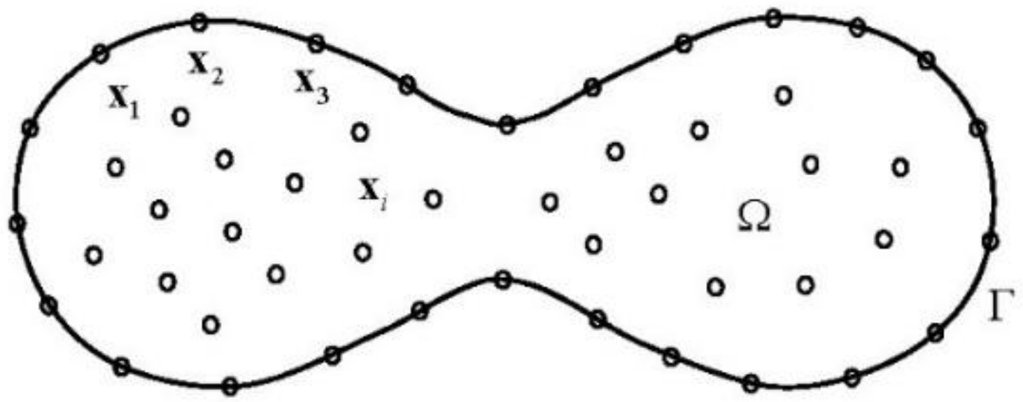
is approximated by
where
are
unknown coefficients at the prescribed points
, which are located in the domain
as well as the boundary
as shown in
Figure 1. Here, it is assumed that
’s are numbered so that the first
points are inside the domain
,
points on
are sequentially numbered and
points on
are lastly numbered with
. In Equation (11), we have defined
and
with
and
being the shape parameter for tuning the numerical accuracy [
17]. When using the approximation (11), polynomials are sometimes augmented to improve the solvability [
21]. In Equations (12) and (13),
is the MQ and
is its particular solution of the Laplace operator as
The
unknown coefficients
can be solved by collocating Equation (11) by the governing Equation (3) and boundary conditions (3) as
where
with
or
gives the differential matrix for the traditional RBFCM and MAPS, respectively. Details have been explicitly addressed in the previous study [
34]. If the system is nonsingular, it can be used for solving the
unknown coefficients
. Sequentially, Equation (11) can be used for approximating
.
For the Hermite MAPS and RBFCM [
20,
21],
is approximated by
with
and
for the Hermite MAPS and RBFCM, respectively. In Equation (17), the subscript
indicates that the differential operators are performed with respect to the source point
as detailed in the literature [
20,
21,
34].
is the MQ particular solution of the biharmonic operator defined by
and
It needs to be mentioned that all of
,
and
are infinitely differentiable [
25]. Similarly, the
unknown coefficients
, in Equation (17), can be solved by collocating the governing Equation (4) and boundary conditions (3) as
where
is the differential matrix for the Hermite MAPS and RBFCM [
34]. Equation (20) is utilized to obtain the
unknown coefficients
with
and
for the Hermite MAPS and RBFCM, respectively. Then, Equation (17) can be used for approximating
of the Hermite methods.
After the solution is obtained by the traditional/Hermite MAPS and RBFCM, the time marching can proceed to a desired final time using Equations (3)–(5).
4. Numerical Results
The traditional/Hermite MAPS and RBFCM are validated by several numerical examples in this section. These examples are essential and natural boundary conditions in rectangular and peanut-shaped domains. Numerical results demonstrate that the Hermite MAPS is the most accurate and stable of these four numerical methods.
In the following analyses, numerical accuracy is evaluated by the maximum absolute error defined by
where
and
are the exact and numerical solutions, respectively. Additionally, it is required that the evaluation points
should be sufficiently dense so that the errors are representative.
4.1. Example 1: Heat Equation (Pure Diffusion)
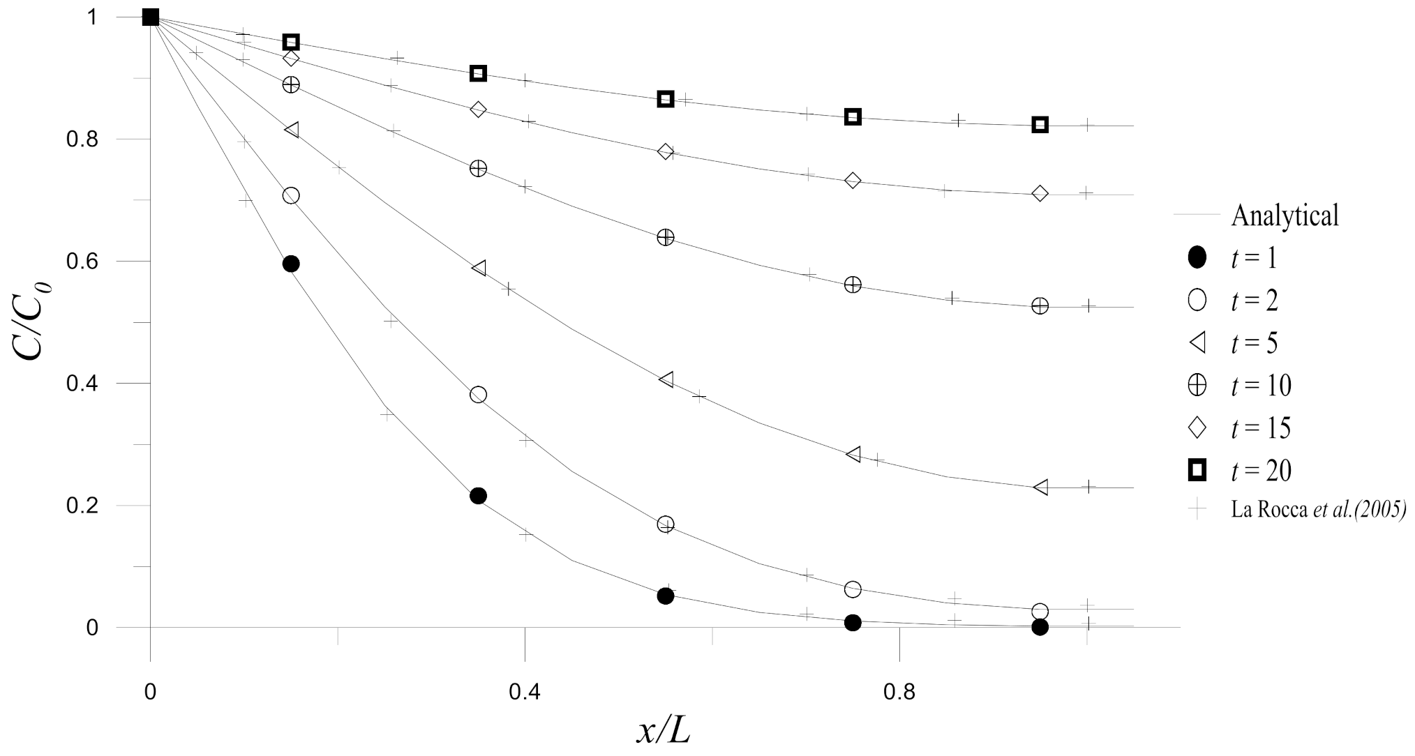
Following La Rocca et al. [
12], we study the solution of the time-dependent heat equation (Equation (1) with
,
, and
) as
with
. A rectangular computational domain
is considered with the following initial and boundary conditions:
and
The analytical solution of the above problem is given by
with
and
In this example, we typically adopt the implicit Euler method (
) with
,
and
if not otherwise mentioned. The Hermite MAPS is validated by solving the prescribed problem and comparing it with the results from the Hermite RBFCM and the analytical solutions as depicted in
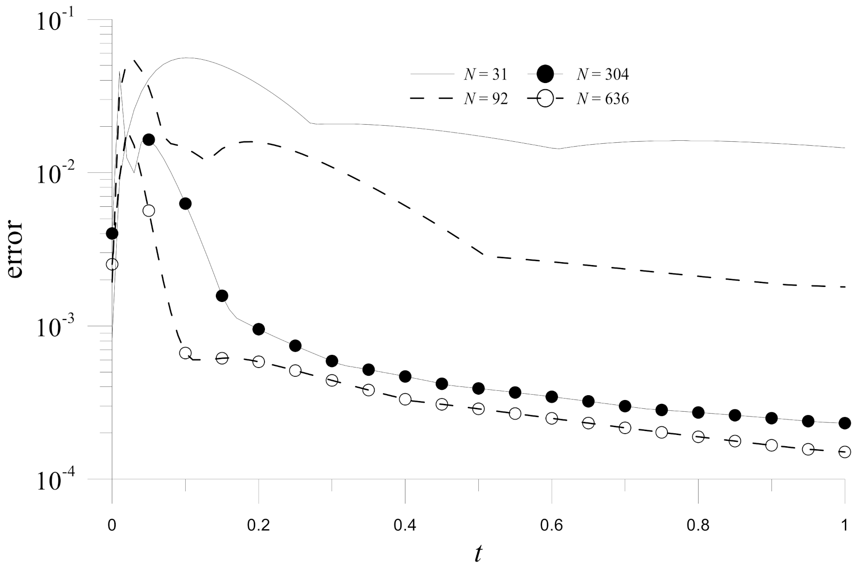
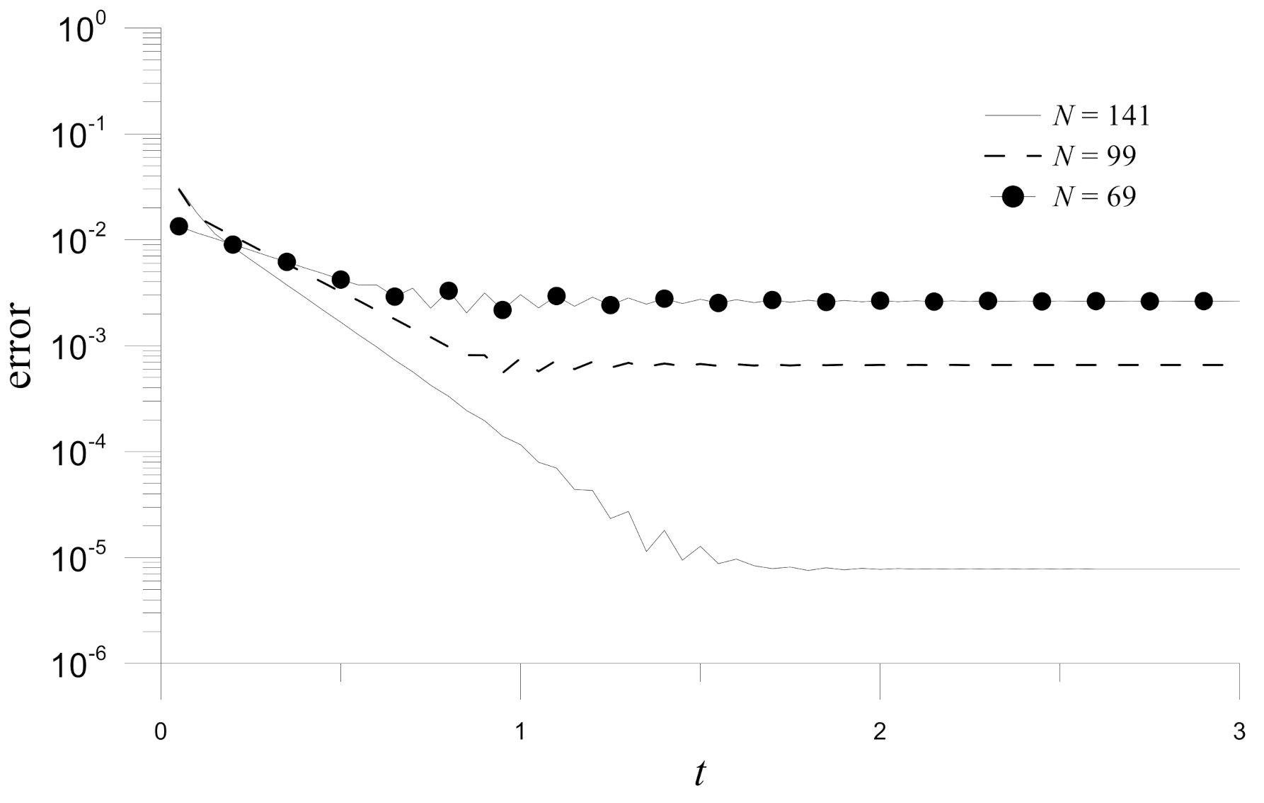
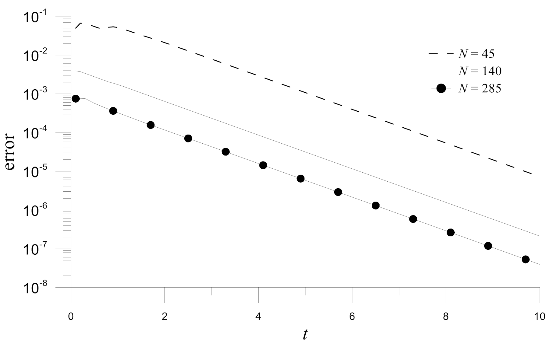
Figure 2. Additionally,
Figure 3 shows the errors obtained by the Hermite MAPS for different node numbers. The convergence concerning the node numbers can be observed.
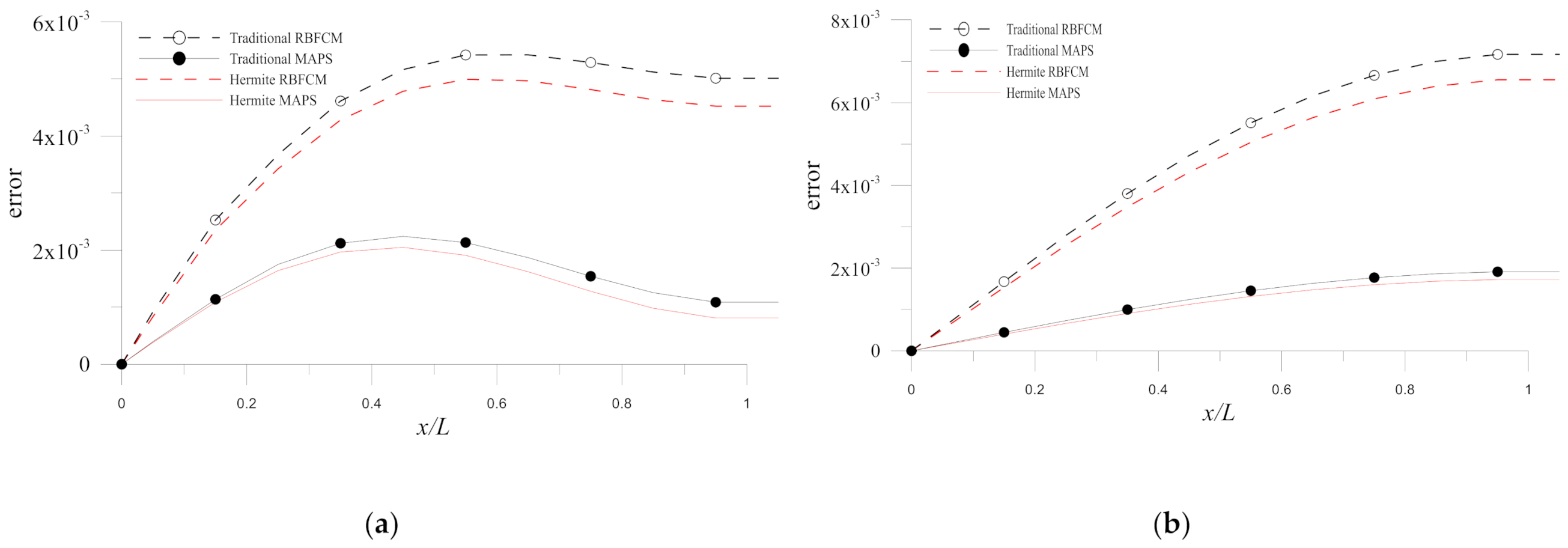
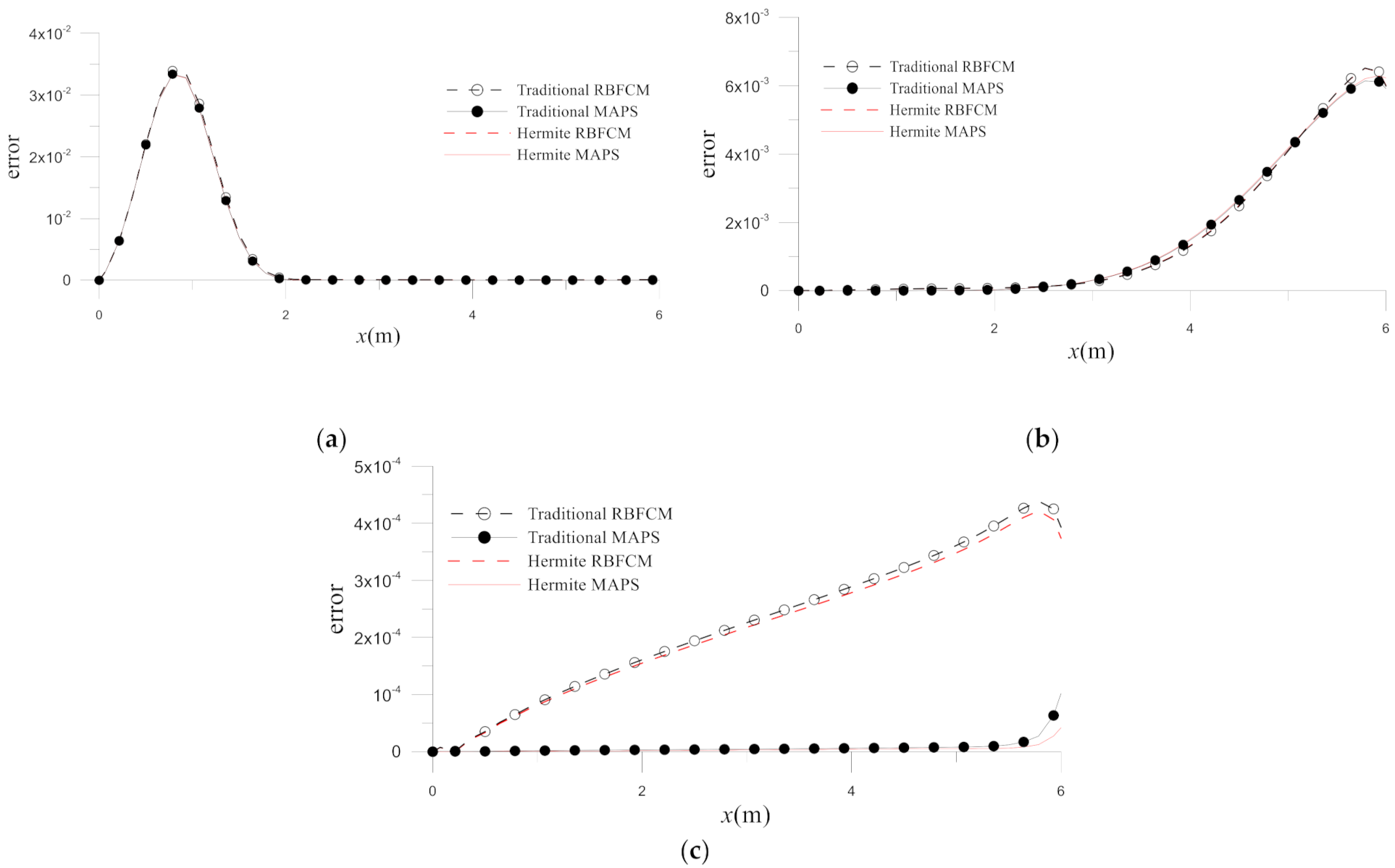
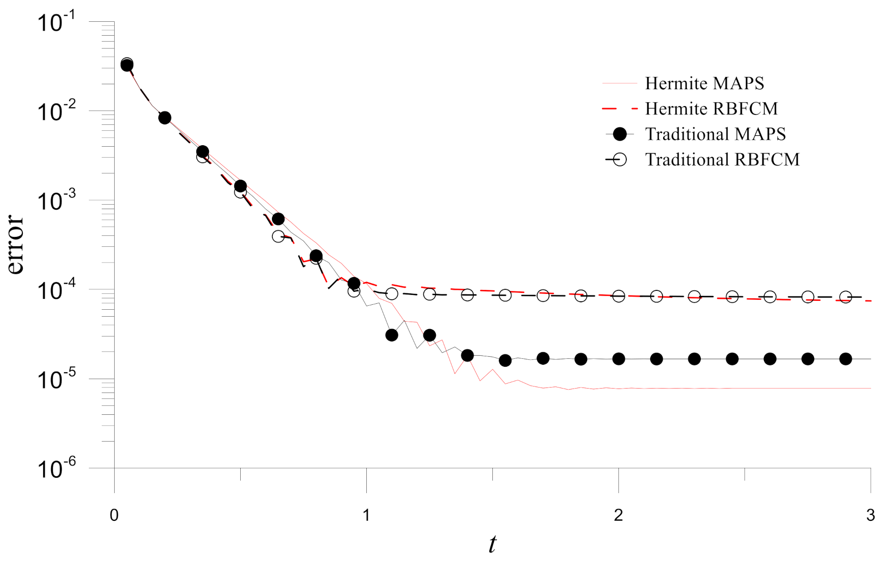
After the Hermite MAPS is validated, comparisons are made between the traditional/Hermite MAPS and RBFCM.
Figure 4 depicts the errors on
at
and
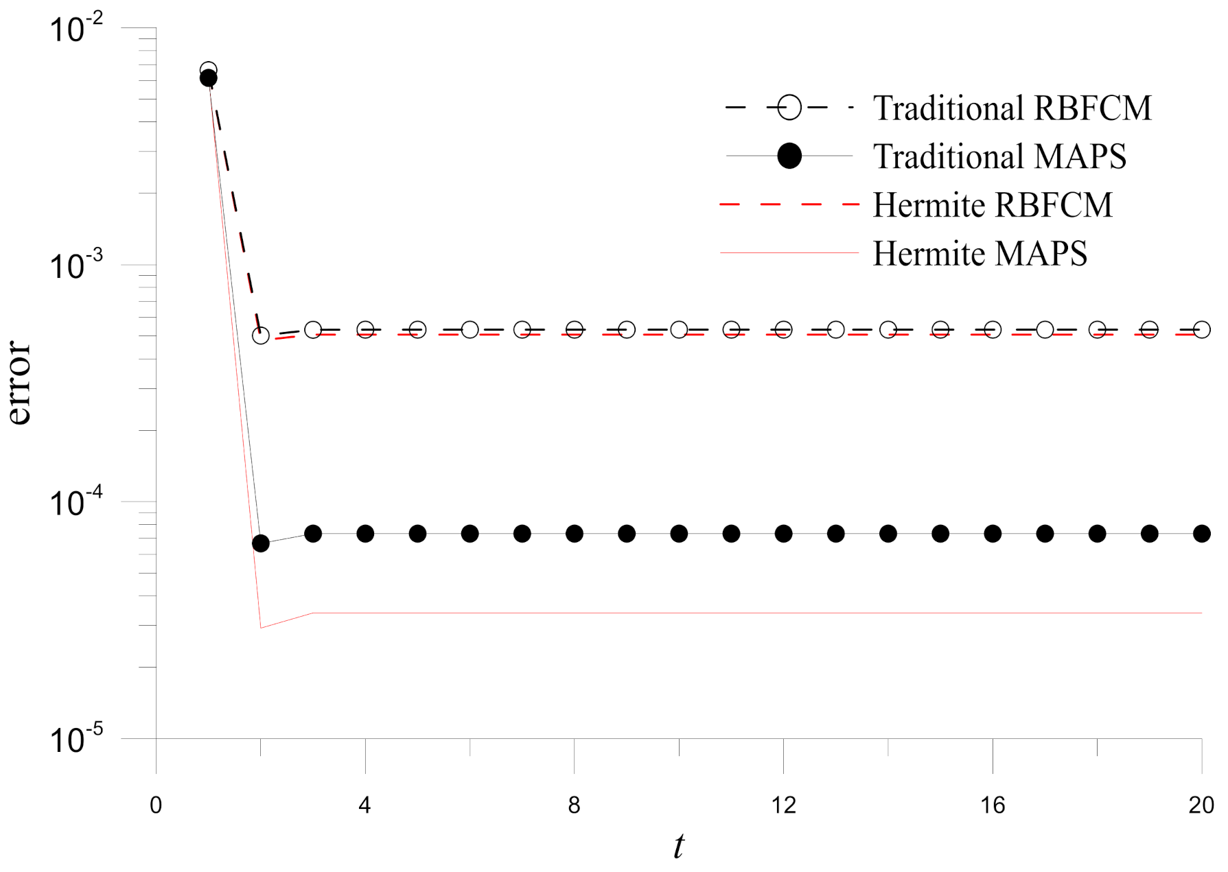
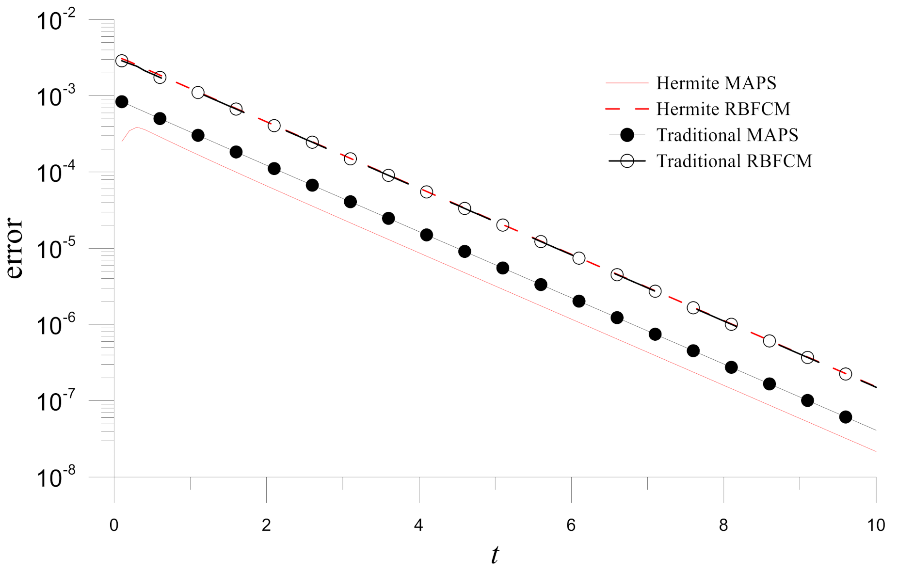
. It is evident from the figure that the MAPS are more accurate, and the Hermite MAPS is the most accurate in these four numerical methods. The accuracy improvement in the Hermite MAPS over the other three methods is further demonstrated by the time histograms of errors for numerical solutions obtained by the four methods (
) in
Figure 5.
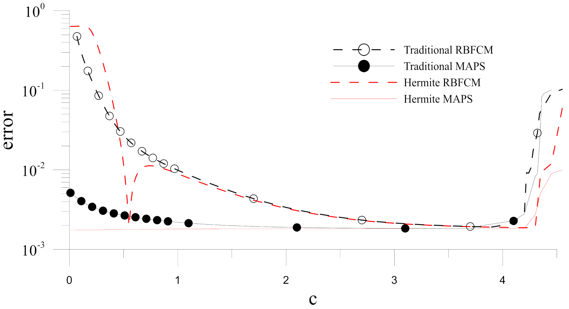
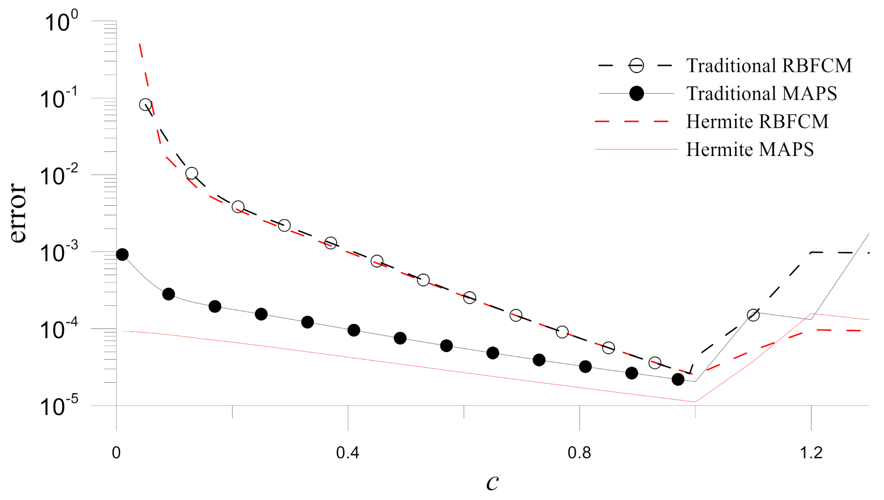
To study the stability of the methods, the numerical errors of the solutions obtained by these four numerical methods are compared for different shape parameters
.
Figure 6 demonstrates the Hermite MAPS is the most stable concerning the shape parameter in these four numerical methods. Additionally, the computing costs for the four methods are studied in
Table 1. In the table, it can be observed that the traditional RBFCM is more efficient than the other three methods. However, the Hermite MAPS is the most time-consuming method, while its computing time is about twice compared with that of the traditional RBFCM. Overall, the computing time by a typical PC is about several minutes in the presented numerical examples.
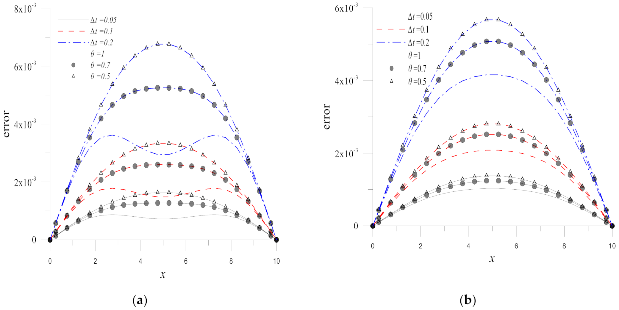
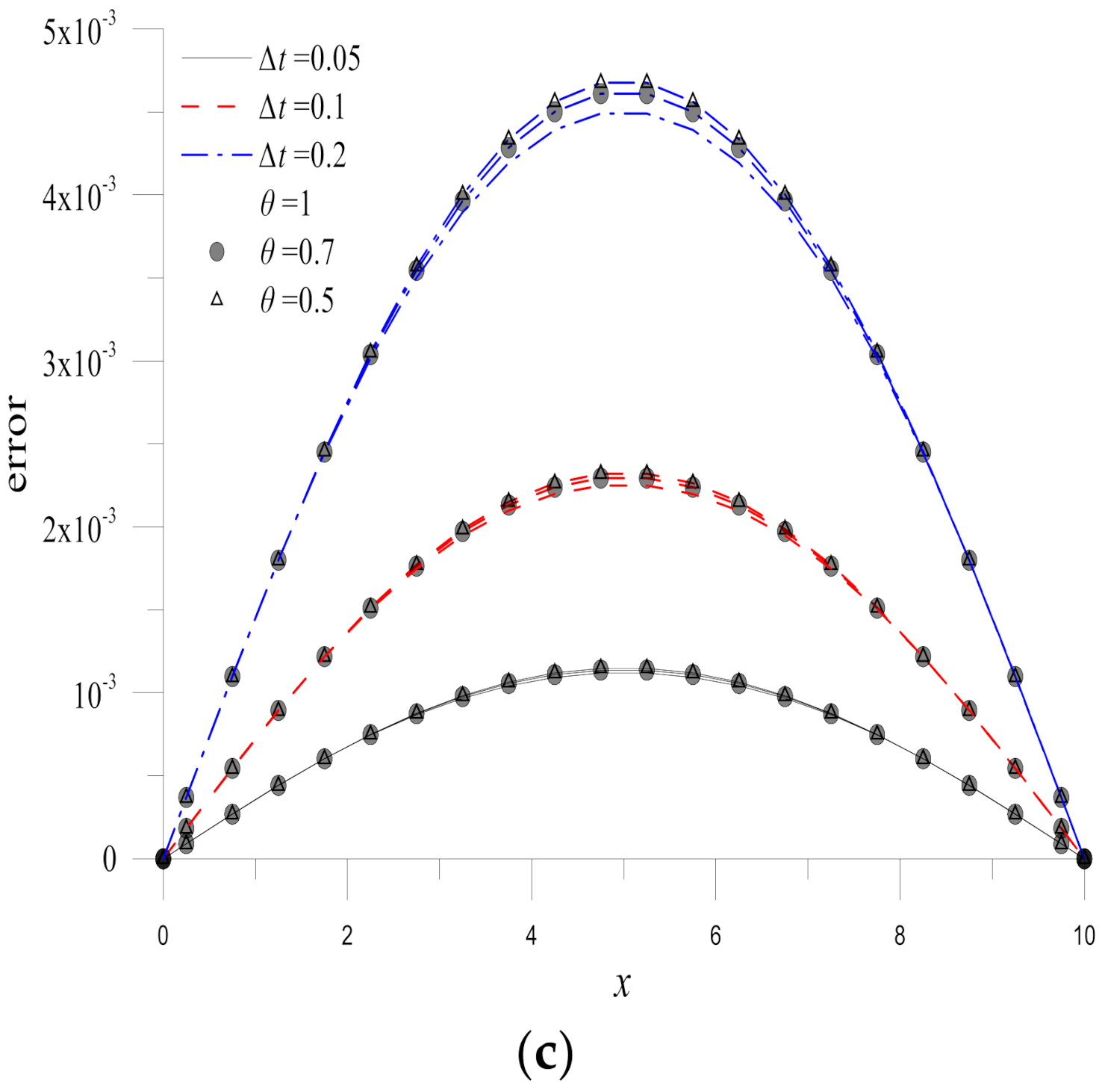
Sequentially, the effects of
and the weighting parameter
are studied as depicted in
Figure 7. The figure shows clearly that the solutions obtained by the methods with smaller
are more accurate. Additionally, the effect of weighting parameter
is not significate while the implicit Euler method (
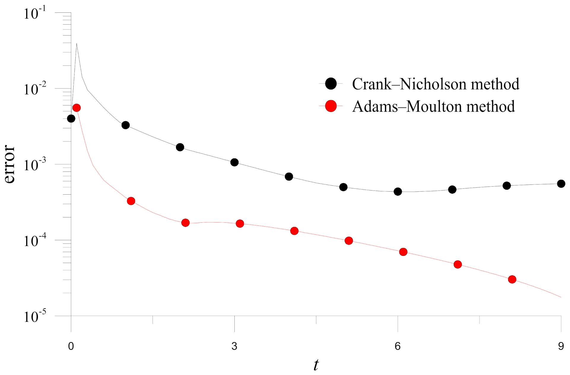
) seems to give slightly more accurate results. Finally, if a more effective temporal discretization is considered, the Adams-Moulton method is applied to solve the present example.
Figure 8 depicts the time histograms of errors obtained by the Crank-Nicholson and Adams-Moulton methods. Significant accuracy improvement in the Adams-Moulton method results can be observed.
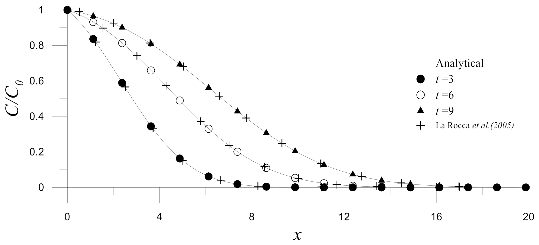
4.2. Example 2: Convective-Diffusion Equation
We consider the solution of the time-dependent convection-diffusion problem with constant diffusion coefficient and convection velocity (Equation (1) with
and
) as
with
and
(Péclet number,
) in a rectangular domain
with initial and boundary conditions as
and
Following La Rocca et al. [
12], the exact solution of the problem is
In this example, numerical results are obtained by using the standard Crank-Nicholson method (
) with
,
and
if not otherwise addressed. Similar to the previous case, the Hermite MAPS is validated by comparing its results with the Hermite RBFCM results and the analytical solutions depicted in
Figure 9. Good agreements can be observed in the figure.
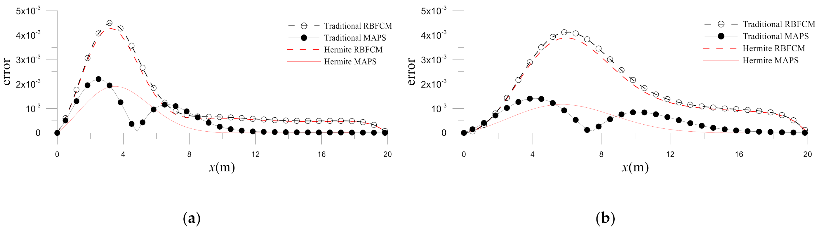
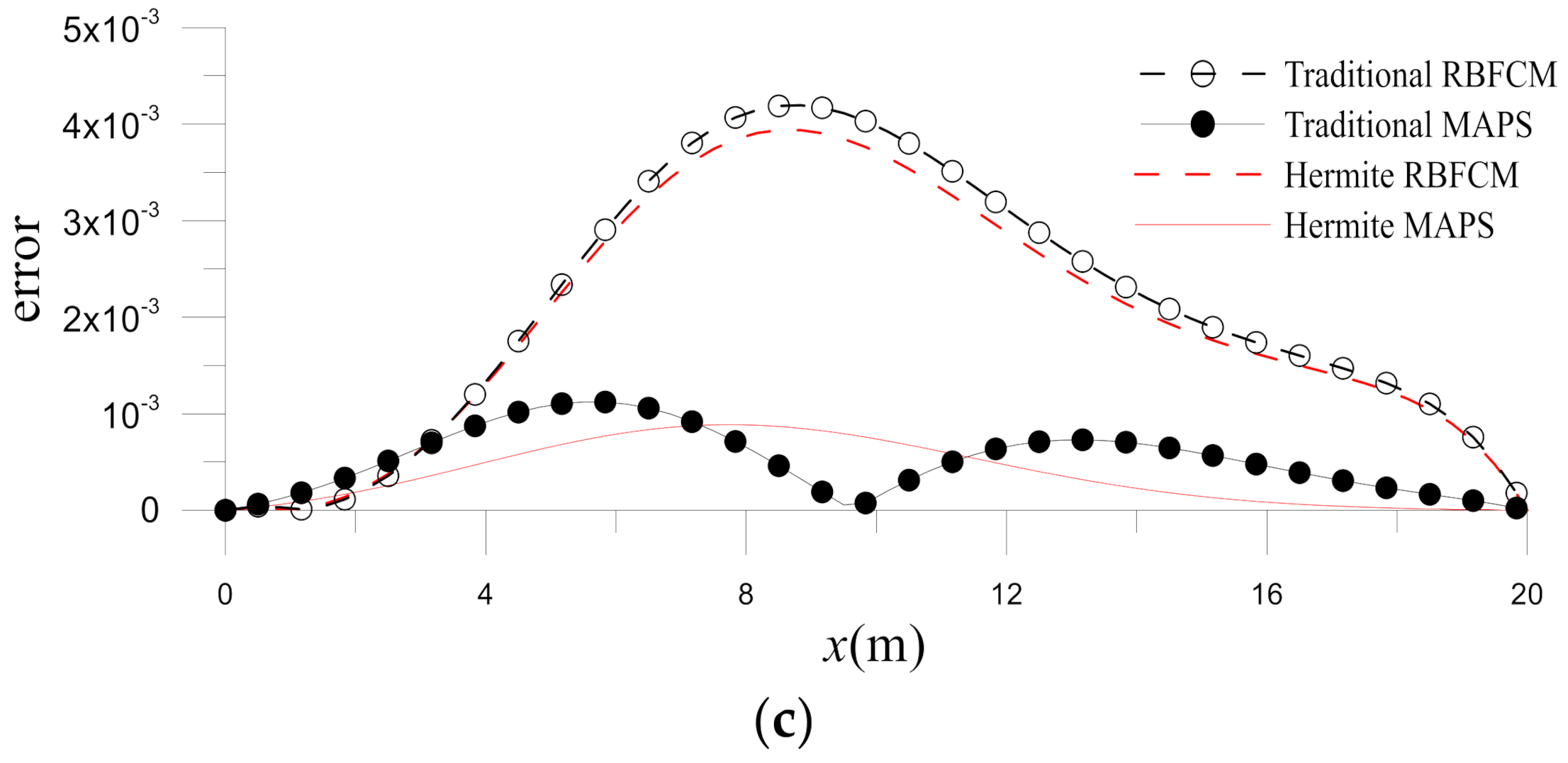
Then, comparisons are made for the traditional/Hermite MAPS and RBFCM.
Figure 10 depicts the errors on
at different times. It is clear from the figure that the MAPS are more accurate. The accuracy improvements are further studied by the time histograms of errors obtained by the four numerical methods.
Figure 11 demonstrates that the Hermite MAPS is the most accurate in these four numerical methods for
.
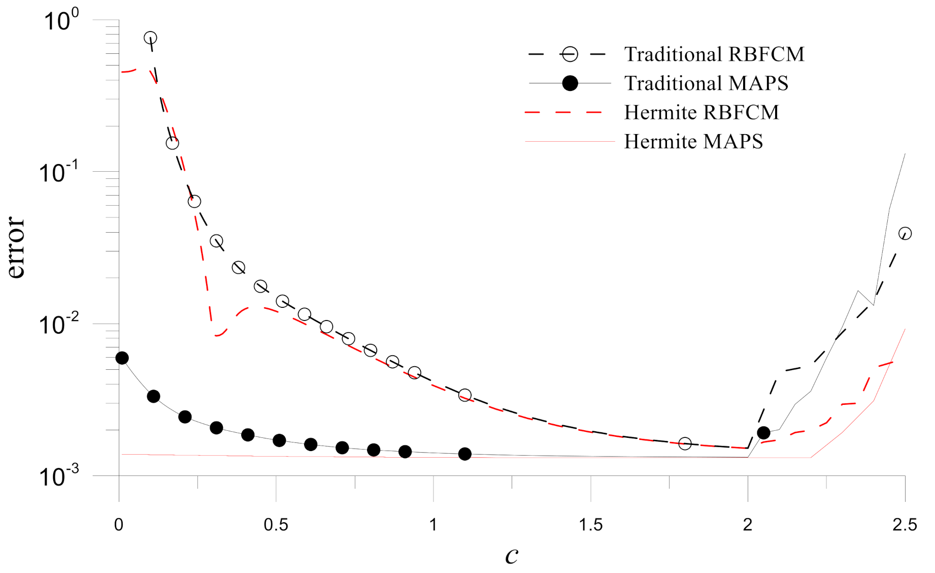
Sequentially, the errors for different shape parameters for the numerical results obtained by the four numerical methods are shown in
Figure 12. The figure also demonstrates that the Hermite MAPS is the most stable concerning the shape parameter in these four numerical methods.
Overall, it is evident that the Hermite MAPS is the most accurate and stable method for solving the present time-dependent convection-diffusion problem.
4.3. Example 3: Convection-Diffusion-Reaction Problem
Following La Rocca et al. [
12], we consider a time-dependent convection-diffusion-reaction problem (Equation (1) with
) as
with
,
, and
(Péclet number,
) in a rectangular domain
. The initial and boundary conditions are given by
and
The exact solution of the problem can be obtained from [
37] as
with
and
In this example, numerical results are obtained by the standard Crank-Nicholson method (
) with
,
and
if not additionally stated. Sequentially, the Hermite MAPS is validated by comparing its results with those obtained by the Hermite RBFCM and the analytical solutions, as shown in
Figure 13. Similar to the previous examples, good agreements can be observed.
The performance of the traditional/Hermite MAPS and RBFCM is then compared.
Figure 14 gives the errors on
at different times and shows that the MAPS are more accurate, especially for a larger time. This result can be expected, as the MAPS contain information from the governing operator. The accuracy improvements are further studied by the time histograms of errors obtained by the four numerical methods. In
Figure 15, it can be found that the Hermite MAPS is the most accurate in these four numerical methods for
.
The stability issue is then studied.
Figure 16 demonstrates the errors for different shape parameters corresponding to the numerical results by the four numerical methods. It also demonstrates that the Hermite MAPS is the most stable concerning the shape parameter in these four numerical methods.
Overall, it is evident the Hermite MAPS is the most accurate and stable method for solving the present time-dependent convection-diffusion-reaction problem.
4.4. Example 4: Time-Dependent Convection-Diffusion-Reaction Problem in a Peanut-Shaped Domain
In order to demonstrate the accuracy and stability outperformance of the Hermite MAPS over the other three methods for problems in irregular domains, we consider the time-dependent convection-diffusion-reaction problem governed by
with
The exact solution of the problem is
with other definitions given in Equations (39) and (40) and parameters the same as those in the previous example. The initial condition is set based on the prescribed analytical solution. Additionally, the essential boundary conditions are enforced on the peanut-shaped boundary defined in polar coordinates
as
The Hermite MAPS is validated by comparing its results with the analytical solutions for different collocation points, as shown in
Figure 17. The convergence concerning the node numbers is also observed. Similarly,
Figure 18 depicts the time histograms of errors obtained by the four numerical methods for
.
Figure 18 demonstrates that Hermite MAPS is the most accurate of these four numerical methods for solving the time-dependent convection-diffusion-reaction problem in the peanut-shaped domain.
4.5. Example 5: Nonlinear Time-Dependent Convection-Diffusion-Reaction Problem
Finally, the Hermite MAPS with the Picard iteration (7) is applied for solving a nonlinear time-dependent convection-diffusion-reaction problem in a square domain of
, which is governed by
with
and
The source term
and the Dirchlet boundary condition are defined according to the exact solution as
The threshold parameter for the convergence criteria of the Picard iteration (8) is set as .
First, the Hermite MAPS is validated by comparing its results with the analytical solutions for different collocation points, as depicted in
Figure 19. An evident convergence concerning the node numbers can be observed. After the Hermite MAPS is validated,
Figure 20 depicts the time histograms of errors obtained by the four numerical methods for
. The figure also shows that the Hermite MAPS is the most accurate among these four numerical methods for solving the nonlinear time-dependent convection-diffusion-reaction problem in the peanut-shaped domain.
Finally, if the more effective Adams-Moulton method is considered,
Figure 21 depicts the time histograms of errors obtained by the Crank-Nicholson and Adams-Moulton methods. Accuracy improvement in the Adams-Moulton method results can also be observed.


