Typed Angularly Decorated Planar Rooted Trees and Ω-Rota-Baxter Algebras

Abstract

As a generalization of Rota–Baxter algebras, the concept of an $\mathsf{\Omega }$-Rota–Baxter could also be regarded as an algebraic abstraction of the integral analysis. In this paper, we introduce the concept of an $\mathsf{\Omega }$-dendriform algebra and show the relationship between $\mathsf{\Omega }$-Rota–Baxter algebras and $\mathsf{\Omega }$-dendriform algebras. Then, we provide a multiplication recursion definition of typed, angularly decorated rooted trees. Finally, we construct the free $\mathsf{\Omega }$-Rota–Baxter algebra by typed, angularly decorated rooted trees.

1. Introduction

1.1. Rota–Baxter Algebras

A Rota–Baxter algebra is an associative algebra equipped with a linear operator that generalizes the algebra of continuous functions with the integral operator. More precisely, for a given commutative ring $\mathbf{k}$ and $\lambda \in \mathbf{k}$, a Rota–Baxter k-algebra of weight $\lambda$ is a k-algebra R, together with a k-linear map $P:R\to R$, such that

$$\begin{array}{c}\hfill P\left(x\right)P\left(y\right)=P\left(P\right(x)y+xP(y)+\lambda xy)\end{array}$$

(1)

for all $x,y\in R.$ Such a linear operator is called a Rota–Baxter operator of weight $\lambda$. The concept of a Rota–Baxter algebra could be regarded as an algebraic framework of the integral analysis. Let R be the $\mathbb{R}$-algebra of continuous function on $\mathbb{R}$. Define $P:R\to R$ as the integration

$$P\left(f\right)\left(x\right):={\int }_0^{x}f\left(t\right)dt.$$

Then, the integration by parts formula

$${\int }_0^{x}P{\left(f\right)}^{\prime }\left(t\right)P\left(g\right)\left(t\right)dt=P\left(f\right)\left(x\right)P\left(g\right)\left(x\right)-{\int }_0^{x}P\left(f\right)\left(t\right)P{\left(g\right)}^{\prime }\left(t\right)dt$$

is just Equation (1) with $\lambda =0$. The concept of Rota–Baxter algebra was introduced in 1960 by Glen Baxter [1] in his probability study of fluctuation theory, and then studied in the 1960s and 1970s by Cartier and Gian-Carlo Rota [2,3,4] in connection with combinatorics. Apparently, this algebra remained inactive until 2000, when new motivations were found, coming from interesting applications in the prominent work of Connes and Kreimer [5] on the renormalization of perturbative quantum field theory, and from the close relationship with the associative Yang–Baxter equation [6] and the construction of free Rota–Baxter algebras related to the shuffle product [7,8]. Since then, the Rota–Baxter operator has appeared in a wide range of areas in mathematics and mathematical physics, such as number theory [9], pre-Lie and Lie algebra [6,10], Hopf algebras [11,12], operads [13], $\mathcal{O}$-operators [14,15], Rota–Baxter groups and skew left braces [16,17], classical Yang–Baxter equations and associative Yang–Baxter equations [14,18].

1.2. Motivations of $\mathsf{\Omega }$-Rota–Baxter Algebras

The study of $\mathsf{\Omega }$-Rota–Baxter algebras was also partly motivated by the formula of partial integrations. Now, we consider the $\mathbb{R}$-algebra of continuous functions on $\mathbb{R}$. Let $\mathsf{\Omega }$ be a nonempty subset of $\mathbb{R}$. Define a set of linear operators $P_{\omega }:R\to R,\omega \in \mathsf{\Omega }$ by the integration

$$P_{\omega }\left(f\right)\left(x\right)={\int }_{\omega }^{x}f\left(t\right)dt.$$

It follows from the formula of partial integration that

$$P_{\alpha }\left(x\right)P_{\beta }\left(y\right)=P_{\alpha }(x{P}_{\beta }\left(y\right)+P_{\alpha }\left(x\right)y),$$

which leads to the emergence of a general notation-$\mathsf{\Omega }$-Rota–Baxter algebras [19]. See Example 1 below.

The second motivation comes from $\mathsf{\Omega }$-operated algebras. The concept of algebras with (one or more) linear operators was introduced by A.G. Kurosch [20]. Later, Guo [21] called such algebras $\mathsf{\Omega }$-operated algebras and constructed their free objects by Motzkin paths, rooted forests and bracketed words.

Definition 1.

Let Ω be a nonempty set. An Ω-operated algebra is an algebra R together with a family of operators $P_{\omega }:R\to R.$

Recently, many scholars have studied multiple operator algebras. Foissy [22,23] studied multiple algebra structure on typed decorated trees. The authors introduced the concepts dendriform family algebras and matching dendriform algebras [24,25,26]. Aguiar [27] introduced some notions of an S-relative algebras in order to provide a simple uniform perspective on these algebras. Ma and Li [28] combined Rota-Baxter family algebras and Hopf $\pi$-(co)algebras, and integrate the Rota-Baxter operator into Hopf $\pi$-(co)algebra, which leads to the concept of Rota-Baxter(Hopf) $\pi$-(co)algebra.

Rooted trees are useful for several areas of mathematics, such as in the study of vector fields [29], numerical analysis [30] and quantum field theory [31]. The work of the British mathematician Cayley in the 1850s can now be considered as the prehistory of pre-Lie algebras. Chapoton and Livernet [32] first showed that the free pre-Lie algebra generated by a set X is given by grafting of X-decorated rooted trees. Recently, typed decorated trees are used by Bruned, Hairer and Zambotti in [33] to give a systematic description of a canonical renormalization procedure of stochastic PDEs. The authors constructed the free dendriform family algebras [26] and the free matching dendriform algebras [24] respectively via typed decorated trees whose vertices are decorated by elements of a set X and edges are decorated by elements of a semigroup $\mathsf{\Omega }$. In this paper, we aim at constructing the free $\mathsf{\Omega }$-Rota-Baxter algebra by typed angularly decorated planar rooted trees.

The outline of this paper. In Section 2, we first recall the concept of $\mathsf{\Omega }$-Rota-Baxter algebras and show that Rota–Baxter algebras induce $\mathsf{\Omega }$-Rota–Baxter algebras. Then, we provide a definition of $\mathsf{\Omega }$-dendriform algebras and prove that $\mathsf{\Omega }$-Rota–Baxter algebras induce $\mathsf{\Omega }$-dendriform algebras. Section 3 is devoted to typed angularly decorated planar rooted trees. We provide a multiplication of typed, angularly decorated planar rooted trees; then, we construct the free $\mathsf{\Omega }$-Rota–Baxter algebras on them.

Notation. Throughout this paper, let $\mathbf{k}$ be a unitary commutative ring, which will be the base ring of all modules, algebras, and linear maps. Algebras are unitary associative algebras but not necessary commutative.

2. Ω-Rota–Baxter Algebras and Ω-Dendriform Algebras

In this section, we first recall $\mathsf{\Omega }$-Rota–Baxter algebras and introduce the concept of $\mathsf{\Omega }$-dendriform algebras. We then construct an $\mathsf{\Omega }$-Rota–Baxter algebra arising from a Rota–Baxter operator of an augmented algebra.

2.1. $\mathsf{\Omega }$-Rota Baxter Algebras

In this section, we mainly investigate some basic properties of Ω-Rota–Baxter algebras.

Definition 2

([19]). Let λ be a given element of k and Ω a nonempty set. An Ω-Rota–Baxter algebra of weight λ, or simple an Ω-RBA of weight λ, is a pair $(R,{\left(P_{\omega }\right)}_{\omega \in \mathsf{\Omega }})$ consisting of an algebra R and a set of linear operators $P_{\omega }:R\to R,\omega \in \mathsf{\Omega }$, that satisfy the Ω-Rota–Baxter equation

$$\begin{array}{c}\hfill P_{\alpha }\left(x\right)P_{\beta }\left(y\right)=P_{\alpha }(x{P}_{\beta }\left(y\right)+P_{\alpha }\left(x\right)y+\lambda xy)forallx,y\in Rand\alpha ,\beta \in \mathsf{\Omega }.\end{array}$$

Any Rota–Baxter algebra of weight λ can be viewed as an Ω-Rota–Baxter algebra of weight λ by taking Ω as a singleton set.

Remark 1.

Another notion of algebras with multiple Rota–Baxter operators, called a Rota–Baxter family algebra, was suggested by Guo in [34]. See also [21,35]. The difference is that, there, the index set Ω is a semigroup and the Rota–Baxter equation in Rota–Baxter family algebras is defined by

$$\begin{array}{c}\hfill P_{\alpha }\left(x\right)P_{\beta }\left(y\right)=P_{\alpha \beta }\left(P_{\alpha }\left(x\right)y\right)+P_{\alpha \beta }\left(x{P}_{\beta }\left(y\right)\right)+\lambda P_{\alpha \beta }\left(xy\right)forx,y\in A,\alpha ,\beta \in \mathsf{\Omega }.\end{array}$$

The following example shows that an $\mathsf{\Omega }$-Rota–Baxter algebra could be regarded as an algebraic framework of the integral analysis, parallel to the fact that a differential algebra could be considered an algebraic abstraction of differential equations.

Example 1

([19]). (Integration (we thank professor L. Guo for suggesting this example)) Let R be the $\mathbb{R}$-algebra of continuous functions on $\mathbb{R}$ and Ω a nonempty subset of $\mathbb{R}$. Define a set of linear operators $P_{\omega }:R\to R,\omega \in \mathsf{\Omega }$ by the integration

$$\begin{array}{c}\hfill P_{\omega }\left(f\right)\left(x\right)={\int }_{\omega }^{x}f\left(t\right)dt.\end{array}$$

Then, the pair $(R,{\left(P_{\omega }\right)}_{\alpha \in \mathsf{\Omega }})$ is an Ω-Rota–Baxter algebra of weight zero. This follows from the integration by parts formula, as follows. For any $f,g\in R,\alpha$ and $\beta \in \mathsf{\Omega }$, set

$$\begin{array}{c}\hfill F\left(x\right):={\int }_{\alpha }^{x}f\left(t\right)dtandG\left(x\right):={\int }_{\beta }^{x}g\left(t\right)dt.\end{array}$$

Then, we have

$$\begin{array}{c}\hfill F\left(\alpha \right)=0,F^{\prime }\left(x\right)=f\left(x\right)and{G}^{\prime }\left(x\right)=g\left(x\right).\end{array}$$

Thus, the integration by parts formula

$$\begin{array}{c}\hfill {\int }_{\alpha }^x{F}^{\prime }\left(t\right)G\left(t\right)dt=F\left(t\right)G\left(t\right){|}_{\alpha }^x-{\int }_{\alpha }^{x}F\left(t\right)G^{\prime }\left(t\right)dt\end{array}$$

can be rewritten as

$$\begin{array}{cc}\hfill {\int }_{\alpha }^{x}f\left(t\right)G\left(t\right)dt=& F\left(t\right)G\left(t\right){|}_{\alpha }^x-{\int }_{\alpha }^{x}F\left(t\right)g\left(t\right)dt\hfill \\ \hfill =& F\left(x\right)G\left(x\right)-F\left(\alpha \right)G\left(\alpha \right)-{\int }_{\alpha }^{x}F\left(t\right)g\left(t\right)dt\hfill \\ \hfill =& F\left(x\right)G\left(x\right)-{\int }_{\alpha }^{x}F\left(t\right)g\left(t\right)dt.\hfill \end{array}$$

In other words,

$$\begin{array}{c}\hfill P_{\alpha }\left(f{P}_{\beta }\left(g\right)\right)\left(x\right)=P_{\alpha }\left(f\right)\left(x\right)P_{\beta }\left(g\right)\left(x\right)-P_{\alpha }\left(P_{\alpha }\left(f\right)g\right)\left(x\right),\end{array}$$

which implies that

$$\begin{array}{c}\hfill P_{\alpha }\left(f{P}_{\beta }\left(g\right)\right)=P_{\alpha }\left(f\right)P_{\beta }\left(g\right)-P_{\alpha }\left(P_{\alpha }\left(f\right)g\right).\end{array}$$

Rearranging the terms, we have

$$\begin{array}{c}\hfill P_{\alpha }\left(f\right)P_{\beta }\left(g\right)=P_{\alpha }\left(f{P}_{\beta }\left(g\right)\right)+P_{\alpha }\left(P_{\alpha }\left(f\right)g\right)forf,g\in R.\end{array}$$

(2)

The following result shows that an $\mathsf{\Omega }$-Rota–Baxter algebra can be constructed from a Rota–Baxter operator of an augmented algebra.

Proposition 1.

Let A be a unitary generalized augmented algebra together with a family of augmentation maps $\alpha :A\to \mathbf{k}$ and Ω a set of augmentation maps. Suppose that P is a Rota–Baxter operator on A. Define

$$\begin{array}{c}\hfill P_{\alpha }\left(x\right):=P\left(x\right)-\alpha \left(P\left(x\right)\right)1forallx\in A,\alpha \in \mathsf{\Omega }.\end{array}$$

Then, $(A,{\left(P_{\alpha }\right)}_{\omega \in \mathsf{\Omega }})$ is an Ω-Rota–Baxter algebra of weight λ.

Proof. 

For any $\alpha ,\beta \in \mathsf{\Omega }$ and $x,y\in A$, we have

$$\begin{array}{cc}\hfill P_{\alpha }\left(x\right)P_{\beta }\left(y\right)& =\left(P\left(x\right)-\alpha \left(P\right(x\left)\right)1\right)\left(P\left(y\right)-\beta \left(P\right(y\left)\right)1\right)\hfill \\ \hfill & =P\left(x\right)P\left(y\right)-P\left(x\right)\beta \left(P\left(y\right)\right)1-\alpha \left(P\left(x\right)\right)1P\left(y\right)+\alpha \left(P\left(x\right)\right)1\beta \left(P\left(y\right)\right)1.\hfill \end{array}$$

Similarly,

$$\begin{array}{cc}\hfill & P_{\alpha }\left(x{P}_{\beta }\left(y\right)+P_{\alpha }\left(x\right)y+\lambda xy\right)\hfill \\ \hfill & =P_{\alpha }(x\left(P\left(y\right)-\beta \left(P\left(y\right)\right)1\right)+P_{\alpha }(\left(P\left(x\right)-\alpha \left(P\left(x\right))1\right)y\right)+\lambda P_{\alpha }\left(xy\right)\hfill \\ \hfill & =P_{\alpha }\left(xP\left(y\right)\right)-\beta \left(P\left(y\right)\right)1P_{\alpha }\left(x\right)+P_{\alpha }\left(P\left(x\right)y\right)-\alpha \left(P\left(x\right)\right)1P_{\alpha }\left(y\right)+\lambda P_{\alpha }\left(xy\right)\hfill \\ \hfill & =P\left(xP\left(y\right)\right)-\alpha \left(P\left(xP\right(y\left)\right)\right)1-\beta \left(P\left(y\right)\right)1\left(P\left(x\right)-\alpha \left(P\left(x\right)\right)1\right)+P\left(P\left(x\right)y\right)-\alpha \left(P\left(P\right(x)y\right)1\hfill \\ \hfill & -\alpha \left(P\left(x\right)\right)1\left(P\left(y\right)-\alpha \left(P\left(y\right)\right)1\right)+\lambda P\left(xy\right)-\alpha \left(P\left(xy\right)\right)1\hfill \\ \hfill & =P\left(x\right)P\left(y\right)-\alpha \left(P\left(xP\right(y\left)\right)\right)1-\beta \left(P\left(y\right)\right)1P\left(x\right)+\beta \left(P\left(y\right)\right)1\alpha \left(P\left(x\right)\right)1\hfill \\ \hfill & -\alpha \left(P\left(P\right(x\left)y\right)\right)1-\alpha \left(P\left(x\right)\right)1P\left(y\right)+\alpha \left(P\left(x\right)\right)1\alpha \left(P\left(y\right)\right)1-\alpha \left(P\left(xy\right)\right)1\hfill \\ \hfill & =P\left(x\right)P\left(y\right)-\alpha \left(P\left(x\right)P\left(y\right)\right)1-\alpha \left(P\left(x\right)\right)1P\left(y\right)\hfill \\ \hfill & +\alpha \left(P\left(x\right)\right)1\alpha \left(P\left(y\right)\right)1-\beta \left(P\left(y\right)\right)1P\left(x\right)+\beta \left(P\left(y\right)\right)1\alpha \left(P\left(x\right)\right)1\hfill \\ \hfill & =P\left(x\right)P\left(y\right)-\alpha \left(P\left(x\right)\right)1P\left(y\right)-\beta \left(P\left(y\right)\right)1P\left(x\right)+\beta \left(P\left(y\right)\right)1\alpha \left(P\left(x\right)\right)1.\hfill \end{array}$$

Thus, we obatin

$$P_{\alpha }\left(x\right)P_{\beta }\left(y\right)=P_{\alpha }\left(x{P}_{\beta }\left(y\right)+P_{\alpha }\left(x\right)y+\lambda xy\right).$$

This completes the proof. □

2.2. $\mathsf{\Omega }$-Dendriform Algebras

In this subsection, we mainly introduce the concept of $\mathsf{\Omega }$-dendriform algebras. Then, we investigate the relationship between $\mathsf{\Omega }$-Rota–Baxter algebras and $\mathsf{\Omega }$-dendriform algebras.

Definition 3.

Let Ω be a nonempty set. An $\mathsf{\Omega }$-dendriform algebra or more precisely an $\mathsf{\Omega }$-multiple dendriform algebra, is a module D together with a family of binary operations ${({\prec }_{\omega },{\succ }_{\omega })}_{\omega \in \mathsf{\Omega }}$, such that, for any $x,y,z\in D$ and $\alpha ,\beta \in \mathsf{\Omega },$ satisfying

$$\left(x{\prec }_{\alpha }y\right){\prec }_{\beta }z=x{\prec }_{\alpha }(y{\prec }_{\beta }z+y{\succ }_{\alpha }z),$$

(3)

$$\left(x{\succ }_{\alpha }y\right){\prec }_{\beta }z=x{\succ }_{\alpha }\left(y{\prec }_{\beta }z\right),$$

(4)

$$x{\succ }_{\alpha }\left(y{\succ }_{\beta }z\right)=(x{\prec }_{\beta }y+x{\succ }_{\alpha }y){\succ }_{\alpha }z.$$

(5)

Definition 4.

Let Ω be a set. An $\mathsf{\Omega }$-tridendriform algebra is a $\mathbf{k}$-module T equipped with a set of linear operations ${({\prec }_{\omega },{\succ }_{\omega })}_{\omega \in \mathsf{\Omega }}$ and a binary operation · such that, for $x,y,z\in T$ and $\alpha ,\beta \in \mathsf{\Omega }$,

$$\begin{array}{c}\hfill \left(x{\prec }_{\alpha }y\right){\prec }_{\beta }z=x{\prec }_{\alpha }(y{\prec }_{\beta }z+y{\succ }_{\alpha }z+y·z),\end{array}$$

(6)

$$\begin{array}{c}\hfill \left(x{\succ }_{\alpha }y\right){\prec }_{\beta }z=x{\succ }_{\alpha }\left(y{\prec }_{\beta }z\right),\end{array}$$

(7)

$$\begin{array}{c}\hfill (x{\prec }_{\beta }y+x{\succ }_{\alpha }y+x·y){\succ }_{\alpha }z=x{\succ }_{\alpha }\left(y{\succ }_{\beta }z\right),\end{array}$$

(8)

$$\begin{array}{c}\hfill \left(x{\succ }_{\alpha }y\right)·z=x{\succ }_{\alpha }(y·z),\end{array}$$

(9)

$$\begin{array}{c}\hfill \left(x{\prec }_{\alpha }y\right)·z=x·\left(y{\succ }_{\alpha }z\right),\end{array}$$

(10)

$$\begin{array}{c}\hfill (x·y){\prec }_{\alpha }z=x·\left(y{\prec }_{\alpha }z\right),\end{array}$$

(11)

$$\begin{array}{c}\hfill (x·y)·z=x·(y·z).\end{array}$$

(12)

As Rota–Baxter family algebras induce (tri)dendriform family algebras [26] and matching Rota–Baxter algebras induce matching dendriform algebras [24], we will prove that $\mathsf{\Omega }$-Rota–Baxter algebras induce the so-called multiple $\mathsf{\Omega }$-dendriform algebras [19].

Proposition 2.

(a)

An Ω-Rota-Baxter algebra $(R,{\left(P_{\omega }\right)}_{\omega \in \mathsf{\Omega }})$ of weight λ induces an Ω-dendriform algebra $(R,{({\prec }_{\omega },{\succ }_{\omega })}_{\omega \in \mathsf{\Omega }})$, where

$$x{\prec }_{\omega }y:=x{P}_{\omega }\left(y\right)+\lambda xy,x{\succ }_{\omega }y:=P_{\omega }\left(x\right)yforx,y\in R,\omega \in \mathsf{\Omega }.$$

(b)

An Ω-Rota-Baxter algebra $(R,{\left(P_{\omega }\right)}_{\omega \in \mathsf{\Omega }})$ of weight 0 induces an Ω-dendriform algebra $(R,{({\prec }_{\omega },{\succ }_{\omega })}_{\omega \in \mathsf{\Omega }})$, where

$$x{\prec }_{\omega }y:=x{P}_{\omega }\left(y\right),x{\succ }_{\omega }y:=P_{\omega }\left(x\right)yforx,y\in R,\omega \in \mathsf{\Omega }.$$

(c)

An Ω-Rota-Baxter algebra $(R,{\left(P_{\omega }\right)}_{\omega \in \mathsf{\Omega }})$ of weight λ induces an Ω-tridendriform algebra $(R,{({\prec }_{\omega },{\succ }_{\omega })}_{\omega \in \mathsf{\Omega }})$, where

$$x{\prec }_{\omega }y:=x{P}_{\omega }\left(y\right),x{\succ }_{\omega }y:=P_{\omega }\left(x\right)y,x·y:=\lambda xyforx,y\in R,\omega \in \mathsf{\Omega }.$$

(d)

An Ω-tridendriform algebra $(T,{({\prec }_{\omega },{\succ }_{\omega })}_{\omega \in \mathsf{\Omega }},·)$ induces two Ω-dendriform algebras $(T,{({\prec }_{\omega }^{\prime },{\succ }_{\omega }^{\prime })}_{\omega \in \mathsf{\Omega }})$ and $(T,{({\prec }_{\omega }^{″},{\succ }_{\omega }^{″})}_{\omega \in \mathsf{\Omega }})$, where

$$\begin{array}{cc}\hfill x{\prec }_{\omega }^{\prime }y:& =x{\prec }_{\omega }y+x·yandx{\succ }_{\omega }^{\prime }y:=x{\succ }_{\omega }y,\hfill \\ \hfill x{\prec }_{\omega }^{″}y:& =x{\prec }_{\omega }yandx{\succ }_{\omega }^{″}y:=x{\succ }_{\omega }y+x·y,forx,y\in T.\hfill \end{array}$$

Proof. 

(a)

For any $\alpha ,\beta \in \mathsf{\Omega }$ and $x,y\in R$, we have

$$\begin{array}{cc}\hfill \left(x{\prec }_{\alpha }y\right){\prec }_{\beta }z& =(x{P}_{\alpha }\left(y\right)+\lambda xy){\prec }_{\beta }z\hfill \\ \hfill & =(x{P}_{\alpha }\left(y\right)+\lambda xy)P_{\beta }\left(z\right)+\lambda (x{P}_{\alpha }\left(y\right)+\lambda xy)z\hfill \\ \hfill & =x{P}_{\alpha }\left(y\right)P_{\beta }\left(z\right)+\lambda xy{P}_{\beta }\left(z\right)+\lambda \left(x{P}_{\beta }\left(y\right)\right)z+{\lambda }^{2}xyz\hfill \\ \hfill & =x{P}_{\alpha }(y{P}_{\beta }\left(z\right)+\lambda yz+P_{\alpha }\left(y\right)z)+\lambda x(y{P}_{\beta }\left(z\right)+\lambda yz+P_{\alpha }\left(y\right)z)\hfill \\ \hfill & =x{\prec }_{\alpha }(y{P}_{\beta }\left(z\right)+\lambda yz+P_{\alpha }\left(y\right)z)\hfill \\ \hfill & =x{\prec }_{\alpha }(y{\prec }_{\beta }z+y{\succ }_{\alpha }z).\hfill \\ \hfill \left(x{\succ }_{\alpha }y\right){\prec }_{\beta }z& =\left(P_{\alpha }\left(x\right)y\right)P_{\beta }\left(z\right)+\lambda \left(P_{\alpha }\left(x\right)y\right)z\hfill \\ \hfill & =P_{\alpha }\left(x\right)(y{P}_{\beta }\left(z\right)+\lambda yz)\hfill \\ \hfill & =(x{\succ }_{\alpha }\left(y{\prec }_{\beta }z\right).\hfill \\ \hfill x{\succ }_{\alpha }\left(y{\succ }_{\beta }z\right)& =P_{\alpha }\left(x\right)\left(P_{\beta }\left(y\right)z\right)=P_{\alpha }\left(x\right)P_{\beta }\left(y\right)z\hfill \\ \hfill & =P_{\alpha }(x{P}_{\beta }\left(y\right)+\lambda xy+P_{\alpha }\left(x\right)y)z\hfill \\ \hfill & =(x{\prec }_{\beta }y+x{\succ }_{\alpha }y){\succ }_{\alpha }z.\hfill \end{array}$$

(b)

This follows from Item (a) by taking $\lambda =0.$

(c)

For $x,y,z\in R$ and $\alpha ,\beta \in \mathsf{\Omega }$, we have

$$\begin{array}{cc}\hfill \left(x{\prec }_{\alpha }y\right){\prec }_{\beta }z& =x{P}_{\alpha }\left(y\right)P_{\beta }\left(z\right)\hfill \\ \hfill & =x(P_{\alpha }\left(y\right)z+y{P}_{\beta }\left(z\right)+\lambda yz)\hfill \\ \hfill & =x{\prec }_{\alpha }(y{\succ }_{\alpha }z+y{\prec }_{\beta }z+y·z).\hfill \\ \hfill \left(x{\succ }_{\alpha }y\right){\prec }_{\beta }z& =P_{\alpha }\left(x\right)y{P}_{\beta }\left(z\right)=x{\succ }_{\alpha }\left(y{\prec }_{\beta }z\right)\hfill \\ \hfill & (x{\prec }_{\beta }y+x{\succ }_{\alpha }y+x·y){\succ }_{\alpha }z\hfill \\ \hfill & =(x{P}_{\beta }\left(y\right)+P_{\alpha }\left(x\right)y+\lambda xy){\succ }_{\alpha }z\hfill \\ \hfill & =P_{\alpha }\left(x\right)P_{\beta }\left(y\right)z=x{\succ }_{\alpha }\left(y{\succ }_{\beta }z\right).\hfill \\ \hfill (x{\prec }_{\beta }y+x{\succ }_{\alpha }y+x·y){\succ }_{\alpha }z& =P_{\alpha }(x{P}_{\beta }\left(y\right)+P_{\alpha }\left(x\right)y+\lambda xy)z\hfill \\ \hfill & =\left(P_{\alpha }\left(x\right)P_{\beta }\left(y\right)\right)z=P_{\alpha }\left(x\right)\left(P_{\beta }\left(y\right)z\right)\hfill \\ \hfill & =x{\succ }_{\alpha }\left(y{\succ }_{\beta }z\right).\hfill \\ \hfill \left(x{\succ }_{\alpha }y\right)·z& =\lambda \left(P_{\alpha }\left(x\right)y\right)z=P_{\alpha }\left(x\right)\left(\lambda yz\right)=x{\succ }_{\alpha }(y·z).\hfill \\ \hfill \left(x{\prec }_{\alpha }y\right)·z& =\lambda \left(x{P}_{\alpha }\left(y\right)\right)z=\lambda x\left(P_{\alpha }\left(y\right)z\right)=x·\left(y{\succ }_{\alpha }z\right).\hfill \\ \hfill (x·y){\prec }_{\alpha }z& =\lambda \left(xy\right)P_{\alpha }\left(z\right)=\lambda x\left(y{P}_{\alpha }\left(z\right)\right)=x·\left(y{\prec }_{\alpha }z\right).\hfill \\ \hfill (x·y)·z& ={\lambda }^2\left(xy\right)z={\lambda }^{2}x\left(yz\right)=x·(y·z).\hfill \end{array}$$

(d)

For $x,y,z\in R$ and $\alpha ,\beta \in \mathsf{\Omega }$, we have

$$\begin{array}{cc}\hfill \left(x{\prec }_{\alpha }^{\prime }y\right){\prec }_{\beta }^{\prime }z& =(x{\prec }_{\alpha }y+x·y){\prec }_{\beta }^{\prime }z\hfill \\ \hfill & =(x{\prec }_{\alpha }y+x·y){\prec }_{\beta }z+(x{\prec }_{\alpha }y+x·y)·z\hfill \\ \hfill & =\left(x{\prec }_{\alpha }y\right){\prec }_{\beta }z+(x·y){\prec }_{\beta }z+\left(x{\prec }_{\alpha }y\right)·z+(x·y)·z\hfill \\ \hfill & =x{\prec }_{\alpha }(y{\prec }_{\beta }z+y{\succ }_{\alpha }z+y·z)+x·(y{\prec }_{\beta }z+y·z+y{\succ }_{\alpha }z).\hfill \\ \hfill & =x{\prec }_{\alpha }^{\prime }(y{\prec }_{\beta }z+y·z+y{\succ }_{\alpha }z)=x{\prec }_{\alpha }^{\prime }(y{\prec }_{\beta }^{\prime }z+y{\succ }_{\alpha }^{\prime }z).\hfill \\ \hfill \left(x{\succ }_{\alpha }^{\prime }y\right){\prec }_{\beta }^{\prime }z& =\left(x{\succ }_{\alpha }y\right){\prec }_{\beta }^{\prime }z=\left(x{\succ }_{\alpha }y\right){\prec }_{\beta }z+\left(x{\succ }_{\alpha }y\right)·z\hfill \\ \hfill & =x{\succ }_{\alpha }(y{\prec }_{\beta }z+y·z)=x{\succ }_{\alpha }^{\prime }\left(y{\prec }_{\beta }^{\prime }z\right).\hfill \\ \hfill x{\succ }_{\alpha }^{\prime }\left(y{\succ }_{\beta }^{\prime }z\right)& =x{\succ }_{\alpha }\left(y{\succ }_{\beta }z\right)=(x{\prec }_{\beta }y+x·y+x{\succ }_{\alpha }y){\succ }_{\alpha }z\hfill \\ \hfill & =(x{\prec }_{\beta }^{\prime }y+x{\succ }_{\alpha }^{\prime }y){\succ }_{\alpha }^{\prime }z.\hfill \end{array}$$

We also have

$$\begin{array}{cc}\hfill \left(x{\prec }_{\alpha }^{″}y\right){\prec }_{\beta }^{″}z& =\left(x{\prec }_{\alpha }y\right){\prec }_{\beta }z\hfill \\ \hfill & =x{\prec }_{\alpha }(y{\prec }_{\beta }z+y{\succ }_{\alpha }z+y·z)\hfill \\ \hfill & =x{\prec }_{\alpha }^{″}(y{\prec }_{\beta }^{″}z+y{\succ }_{\alpha }^{″}z).\hfill \\ \hfill \left(x{\succ }_{\alpha }^{″}y\right){\prec }_{\beta }^{″}z& =(x{\succ }_{\alpha }y+x·y){\prec }_{\beta }z\hfill \\ \hfill & =x{\succ }_{\alpha }\left(y{\prec }_{\beta }z\right)+x·\left(y{\prec }_{\beta }z\right)\hfill \\ \hfill & =x{\succ }_{\alpha }^{″}\left(y{\prec }_{\beta }^{″}z\right).\hfill \\ \hfill \left(x{\succ }_{\alpha }^{″}y\right){\succ }_{\beta }^{″}z& =x{\succ }_{\alpha }^{″}(y{\succ }_{\beta }z+y·z)\hfill \\ \hfill & =(x{\prec }_{\beta }y+x{\succ }_{\alpha }y+x·y){\succ }_{\alpha }z+\left(x{\succ }_{\alpha }y\right)·z+\left(x{\prec }_{\beta }y\right)·z+(x·y)·z\hfill \\ \hfill & =(x{\prec }_{\beta }^{″}y+x{\succ }_{\alpha }^{″}y){\succ }_{\alpha }z+(x{\prec }_{\beta }^{″}y+x{\succ }_{\alpha }^{″}y)·z\hfill \\ \hfill & =(x{\prec }_{\beta }^{″}y+x{\succ }_{\alpha }^{″}y){\succ }_{\alpha }^{″}z.\hfill \end{array}$$

This completes the proof. □

3. Free Ω-Rota–Baxter Algebras on Typed Angularly Decorated Rooted Trees

In this section, we construct free Ω-Rota–Baxter algebras in terms of typed angularly decorated planar rooted trees.

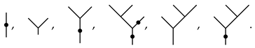
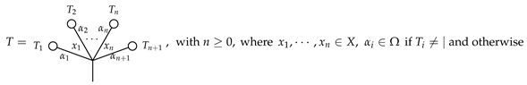
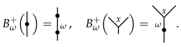
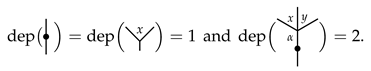
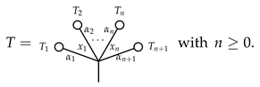
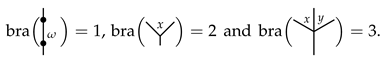
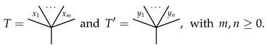
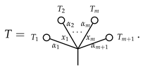
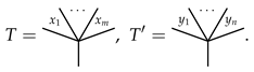
3.1. Typed Angularly Decorated Planar Rooted Trees

First, we recall some notations of planar rooted trees; for more details, see [21,26,36,37]. A $\mathbf{rooted}\mathbf{tree}$ is a finite graph, connected and without cycles, with a special vertex called the $\mathbf{root}$. A $\mathbf{planar}\mathbf{rooted}\mathbf{tree}$ is a rooted tree with a fixed embedding into the plane. The first few planar rooted trees are listed below (note that we view the root and the leaves of a tree as edges rather than vertices):

where the root of a tree is on the bottom.

An edge of a planar rooted tree T is called an inner edge if it is neither a leaf nor the root of T. Let $IE\left(T\right)$ be the set of inner edges of T. For each vertex, v yields a (possibly empty) set of angles $A\left(v\right)$, with an angle being a pair $(e,e^{\prime })$ of adjacent incoming edges for v. Let $A\left(T\right)={\bigsqcup }_{v\in V\left(T\right)}A\left(v\right)$ be the set of angles of T. We now recall the notation of an X-angularly decorated $\mathsf{\Omega }$-typed from [26].

Let X and $\mathsf{\Omega }$ be two sets. An X-angularly decorated $\mathsf{\Omega }$-typed (abbr. typed angularly decorated) planar rooted tree is a planar rooted tree T, together with two maps $\mathrm{dec}:A\left(T\right)\to X$ and $\mathrm{type}:IE\left(T\right)\to \mathsf{\Omega }$. For $n\ge 0$, let $\mathcal{J}(X,\mathsf{\Omega })n$ be the set of X-angularly decorated $\mathsf{\Omega }$-typed planar rooted trees with $n+1$ leaves and define

$$\mathcal{J}(X,\mathsf{\Omega }):=\underset{n\ge 0}{⨆}\mathcal{J}(X,\mathsf{\Omega })n\mathrm{and}\mathbf{k}\mathcal{J}(X,\mathsf{\Omega }):=\underset{n\ge 0}{⨁}\mathbf{k}\mathcal{J}(X,\mathsf{\Omega })n.$$

The following are some examples of X-angularly decorated Ω-typed planar rooted trees in $\mathcal{J}(X,\mathsf{\Omega })$.

Graphically, an element $T\in \mathcal{T}(\mathcal{X},\otimes )$ is of the form:

${\alpha }_i$ does not exist for $1\le i\le n+1$.

For each $\omega \in \mathsf{\Omega }$, there is a grafting operator

$$B_{\omega }^{+}:\mathbf{k}\mathcal{J}(X,\mathsf{\Omega })\to \mathbf{k}\mathcal{J}(X,\mathsf{\Omega })$$

that grafts a tree to a new root and satisfies that the new inner edge between the new root and the root of the tree is typed by $\omega$. For example,

The depth $\mathrm{dep}\left(T\right)$ of a rooted tree T is defined as the maximal length of linear chains from the root to the leaves of the tree. For example,

For later use, we add the “zero-vertex tree” | to the picture, and set $\mathrm{dep}\left(\right|)=0$. For each typed, angularly decorated planar rooted tree T, define the number of branches of T to be $\mathrm{bra}\left(T\right)=0$ if $T=|$. Otherwise, $\mathrm{dep}\left(T\right)\ge 1$ and T is of the form

Here, any branch $T_j\in \mathcal{J}(X,\mathsf{\Omega })\bigsqcup \left\{\right|\},j=1,\dots ,n+1$ is of a depth that is, at most, one less than the depth of T, and equal to zero if, and only if, $T_j=|$. We define $\mathrm{bra}\left(T\right):=n+1$. For example,

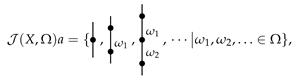
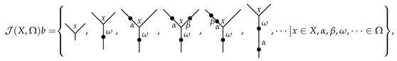
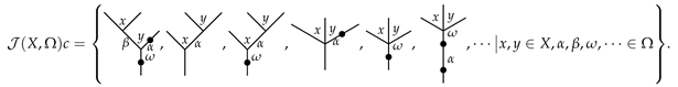
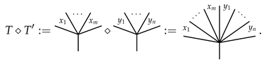
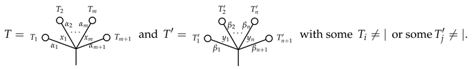
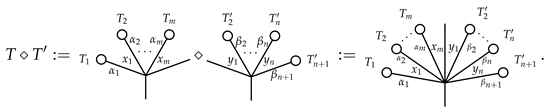
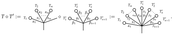
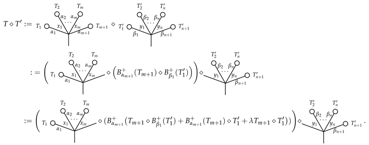
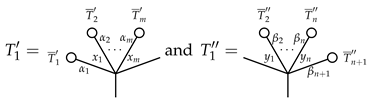
3.2. The Product ⋄ on Typed Angularly Decorated Planar Rooted Trees

Let X be a set and let $\mathsf{\Omega }$ be a set. We now define a product ⋄ on $\mathbf{k}\mathcal{J}(X,\mathsf{\Omega })$ by induction. For $T,T^{\prime }\in \mathcal{J}(X,\mathsf{\Omega })$, we define $T\diamond T^{\prime }$ by induction on $\mathrm{dep}\left(T\right)+\mathrm{dep}\left(T^{\prime }\right)\ge 2$. For the initial step $\mathrm{dep}\left(T\right)+\mathrm{dep}\left(T^{\prime }\right)=2$, we have $\mathrm{dep}\left(T\right)=\mathrm{dep}\left(T^{\prime }\right)=1$ and $T,T^{\prime }$ are of the form

Define

(13)

For the induction step $\mathrm{dep}\left(T\right)+\mathrm{dep}\left(T^{\prime }\right)\ge 3$, the trees T and $T^{\prime }$ are of the form

There are four cases to consider.

Case 1:$T_{m+1}=|=T_1^{\prime }$. Define

(14)

Case 2:$T_{m+1}\ne |=T_1^{\prime }$. Define

(15)

Case 3:$T_{m+1}=|\ne T_1^{\prime }$. Define

(16)

Case 4:$T_{m+1}\ne |\ne T_1^{\prime }$. Define

(17)

Here, the first ⋄ is defined by Case 3, the second, third and fourth ⋄ are defined by induction and the last ⋄ is defined by Case 2. This completes the inductive definition of the multiplication ⋄ on $\mathcal{J}(X,\mathsf{\Omega })$. Extending by linearity, we can expand the ⋄ to $\mathbf{k}\mathcal{J}(X,\mathsf{\Omega })$. Now, we have the following result.

Example 2.

Let X be a set and Ω a nonempty set. For $\alpha ,\beta \in \mathsf{\Omega },$ and $x,y\in X$, we have

Lemma 1.

Let Ω be a set. Then $(\mathbf{k}\mathcal{J}(X,\mathsf{\Omega }),\diamond ,{\left(B_{\omega }^{+}\right)}_{\omega \in \mathsf{\Omega }})$ is an Ω-Rota-Baxter algebra.

Proof. 

We prove that $(\mathbf{k}\mathcal{J}(X,\mathsf{\Omega }),\diamond ,{\left(B_{\omega }^{+}\right)}_{\omega \in \mathsf{\Omega }})$ is an $\mathsf{\Omega }$-Rota–Baxter algebra. From Case 4, when $m=n=0$, we immediately obtain ${\left(B_{\omega }^{+}\right)}_{\omega \in \mathsf{\Omega }}$, satisfying the $\mathsf{\Omega }$-Rota–Baxter equation. By the construction of $\mathbf{k}\mathcal{J}(X,\mathsf{\Omega })$ is closed under ⋄ and is the identity of ⋄.

Now, we show the associativity of ⋄, i.e.

$$\begin{array}{c}\hfill (T_1\diamond T_2)\diamond T_3=T_1\diamond (T_2\diamond T_3)\mathrm{for}\mathrm{all}{T}_1,T_2,T_3\in \mathcal{J}(X,\mathsf{\Omega }).\end{array}$$

(18)

We prove Equation (18) by induction on the sum of depths $p:=\mathrm{dep}\left(T_1\right)+\mathrm{dep}\left(T_2\right)+\mathrm{dep}\left(T_3\right)$. If $p=3$, then $\mathrm{dep}\left(T_1\right)=\mathrm{dep}\left(T_2\right)=\mathrm{dep}\left(T_3\right)=1$ and $T_1,T_2,T_3$ are of the form

Then $(T_1\diamond T_2)\diamond T_3=T_1\diamond (T_2\diamond T_3)$ by direct calculation.

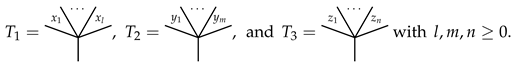
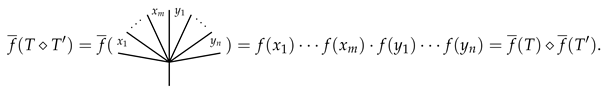
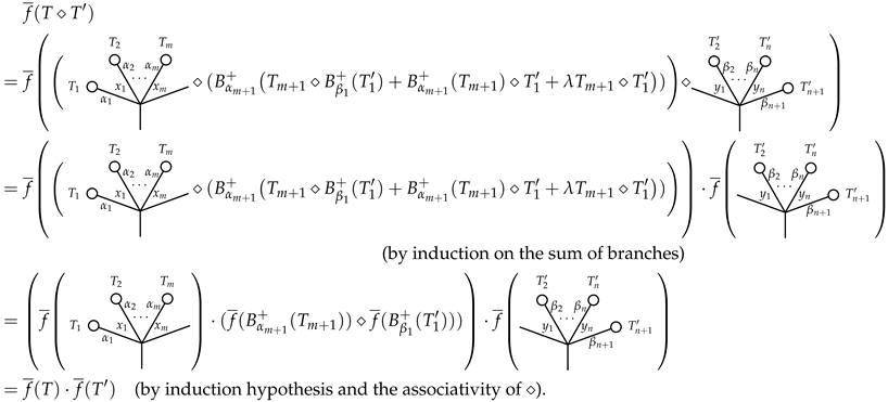
If $p>3$, we use induction on the sum of branches $q:=\mathrm{bra}\left(T_1\right)+\mathrm{bra}\left(T_2\right)+\mathrm{bra}\left(T_3\right)$. If $q=3$ and one of $T_1,T_2,T_3$ has depth 1, then this tree must be of the form and the associativity of ⋄ follows directly. Assume

$$\begin{array}{c}\hfill T_1=B_{\alpha }^{+}\left(T_1^{\prime }\right),T_2=B_{\beta }^{+}\left(T_2^{\prime }\right),T_3=B_{\gamma }^{+}\left(T_3^{\prime }\right)\mathrm{for}\mathrm{some}\alpha ,\beta ,\gamma \in \mathsf{\Omega }\mathrm{and}{T}_1^{\prime },T_2^{\prime },T_3^{\prime }\in \mathcal{J}(X,\mathsf{\Omega }),\end{array}$$

then

$$\begin{array}{cc}\hfill & (T_1\diamond T_2)\diamond T_3=\left(B_{\alpha }^{+}\left(T_1^{\prime }\right)\diamond B_{\beta }^{+}\left(T_2^{\prime }\right)\right)\diamond B_{\gamma }^{+}\left(T_3^{\prime }\right)\hfill \\ \hfill =& B_{\alpha }^{+}\left(T_1^{\prime }\diamond B_{\beta }^{+}\left(T_2^{\prime }\right)+B_{\alpha }^{+}\left(T_1^{\prime }\right)\diamond T_2^{\prime }+\lambda T_1^{\prime }\diamond T_2^{\prime }\right)\diamond B_{\gamma }^{+}\left(T_3^{\prime }\right)\hfill \\ \hfill =& B_{\alpha }^{+}((T_1^{\prime }\diamond B_{\beta }^{+}\left(T_2^{\prime }\right))\diamond B_{\gamma }^{+}\left(T_3^{\prime }\right)+(B_{\alpha }^{+}\left(T_1^{\prime }\right)\diamond T_2^{\prime })\diamond B_{\gamma }^{+}\left(T_3^{\prime }\right)+\lambda (T_1^{\prime }\diamond T_2^{\prime })\diamond B_{\gamma }^{+}\left(T_3^{\prime }\right)\hfill \\ \hfill & +B_{\alpha }^{+}(T_1^{\prime }\diamond B_{\beta }^{+}\left(T_2^{\prime }\right))\diamond T_3^{\prime }+B_{\alpha }^{+}(B_{\alpha }^{+}\left(T_1^{\prime }\right)\diamond T_2^{\prime })\diamond T_3^{\prime }+\lambda B_{\alpha }^{+}(T_1^{\prime }\diamond T_2^{\prime })\diamond T_3^{\prime }+\lambda (T_1^{\prime }\diamond B_{\beta }^{+}\left(T_2^{\prime }\right))\diamond T_3^{\prime }\hfill \\ \hfill & +\lambda (B_{\alpha }^{+}\left(T_1^{\prime }\right)\diamond T_2^{\prime })\diamond T_3^{\prime }+{\lambda }^2(T_1^{\prime }\diamond T_2^{\prime })\diamond T_3^{\prime })\hfill \\ \hfill =& B_{\alpha }^{+}(T_1^{\prime }(B_{\beta }^{+}\left(T_2^{\prime }\right)\diamond B_{\gamma }^{+}\left(T_3^{\prime }\right)+B_{\alpha }^{+}\left(T_1^{\prime }\right)\diamond (T_2^{\prime }\diamond B_{\gamma }^{+}\left(T_3^{\prime }\right))+\lambda T_1^{\prime }\diamond (T_2^{\prime }\diamond B_{\gamma }^{+}\left(T_3^{\prime }\right))\hfill \\ \hfill & +B_{\alpha }^{+}(T_1^{\prime }\diamond B_{\beta }^{+}\left(T_2^{\prime }\right))\diamond T_3^{\prime }+B_{\alpha }^{+}(B_{\alpha }^{+}\left(T_1^{\prime }\right)\diamond T_2^{\prime })\diamond T_3^{\prime }+\lambda B_{\alpha }^{+}(T_1^{\prime }\diamond T_2^{\prime })\diamond T_3^{\prime }+\lambda T_1^{\prime }\diamond (B_{\beta }^{+}\left(T_2^{\prime }\right)\diamond T_3^{\prime })\hfill \\ \hfill & +\lambda B_{\alpha }^{+}\left(T_1^{\prime }\right)\diamond (T_2^{\prime }\diamond T_3^{\prime })+{\lambda }^2{T}_1^{\prime }\diamond (T_2^{\prime }\diamond T_3^{\prime }))\hfill \\ \hfill & (\mathrm{by}\mathrm{induction}\mathrm{hypothesis})\hfill \\ \hfill =& B_{\alpha }^{+}(T_1^{\prime }\diamond B_{\beta }^{+}(T_2^{\prime }\diamond B_{\gamma }^{+}\left(T_3^{\prime }\right))+T_1^{\prime }\diamond B_{\beta }^{+}(B_{\beta }^{+}\left(T_2^{\prime }\right)\diamond T_3^{\prime })+\lambda T_1^{\prime }\diamond B_{\beta }^{+}(T_2^{\prime }\diamond T_3^{\prime })\hfill \\ \hfill & +B_{\alpha }^{+}\left(T_1^{\prime }\right)\diamond (T_2^{\prime }\diamond B_{\gamma }^{+}\left(T_3^{\prime }\right))+B_{\alpha }^{+}\left(T_1^{\prime }\right)\diamond (B_{\beta }^{+}\left(T_2^{\prime }\right)\diamond T_3^{\prime })+\lambda B_{\alpha }^{+}\left(T_1^{\prime }\right)\diamond (T_2^{\prime }\diamond T_3^{\prime })+\lambda T_1^{\prime }\diamond (T_2^{\prime }\diamond B_{\gamma }^{+}\left(T_3^{\prime }\right))\hfill \\ \hfill & +\lambda T_1^{\prime }\diamond (B_{\beta }^{+}\left(T_2^{\prime }\right)\diamond T_3^{\prime })+{\lambda }^2{T}_1^{\prime }\diamond (T_2^{\prime }\diamond T_3^{\prime }))\hfill \\ \hfill =& B_{\alpha }^{+}\left(T_1^{\prime }\right)\diamond B_{\beta }^{+}\left(T_2^{\prime }\diamond B_{\gamma }^{+}\left(T_3^{\prime }\right)+B_{\beta }^{+}\left(T_2^{\prime }\right)\diamond T_3^{\prime }+\lambda T_2^{\prime }\diamond T_3^{\prime }\right)\hfill \\ \hfill =& B_{\alpha }^{+}\left(T_1^{\prime }\right)\diamond (B_{\beta }^{+}\left(T_2^{\prime }\right)\diamond B_{\gamma }^{+}\left(T_3^{\prime }\right))=T_1\diamond (T_2\diamond T_3).\hfill \end{array}$$

If $m>3$, then at least one of $T_1,T_2,T_3$ have branches greater than or equal to 2. If $\mathrm{bra}\left(T_1\right)\ge 2$, then there are $T_1^{\prime },T_1^{″}$ of the form

such that $T_1=T_1^{\prime }\diamond T_1^{″}$. Hence

$$\begin{array}{cc}\hfill & (T_1\diamond T_2)\diamond T_3=((T_1^{\prime }\diamond T_1^{″})\diamond T_2)\diamond T_3\hfill \\ \hfill =& (T_1^{\prime }\diamond (T_1^{″}\diamond T_2))\diamond T_3(\mathrm{By}\mathrm{induction}\mathrm{hypothesis})\hfill \\ \hfill =& T_1^{\prime }\diamond ((T_1^{″}\diamond T_2)\diamond T_3)(\mathrm{By}\mathrm{the}\mathrm{form}\mathrm{of}{T}_1^{\prime }\mathrm{and}\mathrm{the}\mathrm{definition}\mathrm{of}\diamond )\hfill \\ \hfill =& T_1^{\prime }\diamond (T_1^{″}\diamond (T_2\diamond T_3)(\mathrm{By}\mathrm{induction}\mathrm{hypothesis})\hfill \\ \hfill =& T_1^{\prime }\diamond T_1^{″}\diamond (T_2\diamond T_3)(\mathrm{By}\mathrm{the}\mathrm{form}\mathrm{of}{T}_1^{\prime }\mathrm{and}\mathrm{the}\mathrm{definition}\mathrm{of}\diamond )\hfill \\ \hfill =& T_1\diamond (T_2\diamond T_3).\hfill \end{array}$$

If $\mathrm{bra}\left(T_2\right)\ge 2$ or $\mathrm{bra}\left(T_3\right)\ge 2$, the associativity can be similarly proved. □

Let $i:X\to \mathbf{k}\mathcal{J}(X,\mathsf{\Omega }),i\left(x\right)=$ be a set map. Then, we have the following result.

Proposition 3.

Let Ω be a set. $(\mathbf{k}\mathcal{J}(X,\mathsf{\Omega }),\diamond ,{\left(B_{\omega }^{+}\right)}_{\omega \in \mathsf{\Omega }})$ together with the map i is the free Ω-Rota–Baxter algebra generated by X.

Proof. 

By Lemma 1 and the definition of ⋄, $(\mathbf{k}\mathcal{J}(X,\mathsf{\Omega }),\diamond ,{\left(B_{\omega }^{+}\right)}_{\omega \in \mathsf{\Omega }})$ is an $\mathsf{\Omega }$-Rota–Baxter algebra. Now, we show the freeness of $\mathbf{k}\mathcal{J}(X,\mathsf{\Omega })$.

Let $(A,·,{\left(P_{\omega }\right)}_{\omega \in \mathsf{\Omega }})$ be an $\mathsf{\Omega }$-Rota–Baxter algebra and $f:X\to A$ a set map. We extend f to an $\mathsf{\Omega }$-Rota–Baxter algebra morphism $\overline{f}:\mathbf{k}\mathcal{J}(X,\mathsf{\Omega })\to A$ as follows: For $T\in \mathcal{J}(X,\mathsf{\Omega })$, we define $\overline{f}\left(T\right)$ by induction on $\mathrm{dep}\left(T\right)$. If $\mathrm{dep}\left(T\right)=1$, then T is of the form

Define $\overline{f}\left(T\right):=f\left(x_1\right)·f\left(x_2\right)\cdots f\left(x_m\right)$. Suppose $\overline{f}\left(T\right)$ was defined for all trees of depth $\le k$, where $k\ge 1$ is a fixed integer. Consider the case of $\mathrm{dep}\left(T\right)=k+1$, we define $\overline{f}\left(T\right)$ by induction on the branches of T. If $\mathrm{bra}\left(T\right)=1$, then T is of the form

Define

$$\overline{f}\left(T\right):=P_{\omega }(P_{{\alpha }_1}\left(\overline{f}\left(T_1\right)\right)·f\left(x_1\right)·P_{{\alpha }_2}\left(\overline{f}\left(T_2\right)\right)\cdots P_{{\alpha }_m}\left(\overline{f}\left(T_m\right)\right)·f\left(x_m\right)·P_{{\alpha }_{m+1}}\left(\overline{f}\left(T_{m+1}\right)\right)).$$

If $\mathrm{bra}\left(T\right)>1$, then T is of the form

Define

$$\overline{f}\left(T\right):=P_{{\alpha }_1}\left(\overline{f}\left(T_1\right)\right)·f\left(x_1\right)·P_{{\alpha }_2}\left(\overline{f}\left(T_2\right)\right)\cdots P_{{\alpha }_m}\left(\overline{f}\left(T_m\right)\right)·f\left(x_m\right)·P_{{\alpha }_{m+1}}\left(\overline{f}\left(T_{m+1}\right)\right).$$

By the construction of $\overline{f}$, $P_{\omega }\overline{f}=\overline{f}{B}_{\omega }^{+}$ for all $\omega \in \mathsf{\Omega }$. Next, we show that $\overline{f}$ is an algebra homomorphism, i.e.,

$$\begin{array}{c}\hfill \overline{f}(T\diamond T^{\prime })=\overline{f}\left(T\right)·\overline{f}\left(T^{\prime }\right)\mathrm{for}\mathrm{all}T,T^{\prime }\in \mathcal{J}(X,\mathsf{\Omega }).\end{array}$$

(19)

We prove that Equation (19) holds by induction on the sum of depth $\mathrm{dep}\left(T\right)+\mathrm{dep}\left(T^{\prime }\right)\ge 2$. If $\mathrm{dep}\left(T\right)+\mathrm{dep}\left(T^{\prime }\right)=2$, then $\mathrm{dep}\left(T\right)=\mathrm{dep}(\left(T^{\prime }\right)=1$ and

Then

Assume that Equation (19) holds when $\mathrm{dep}\left(T\right)+\mathrm{dep}\left(T^{\prime }\right)\le k$ for a given $k\ge 2$ and consider the case of $\mathrm{dep}\left(T\right)+\mathrm{dep}\left(T^{\prime }\right)=k+1$. We reduce to the induction on $\mathrm{bra}\left(T\right)+\mathrm{bra}\left(T^{\prime }\right)$. For the initial step of $\mathrm{bra}\left(T\right)+\mathrm{bra}\left(T^{\prime }\right)=2$, we have $\mathrm{bra}\left(T\right)=\mathrm{bra}\left(T^{\prime }\right)=1$ and $T=B_{\alpha }^{+}\left(T_1\right),T^{\prime }=B_{\beta }^{+}\left(T_1^{\prime }\right)$. Then

$$\begin{array}{cc}\hfill & \overline{f}(T\diamond T^{\prime })=\overline{f}(B_{\alpha }^{+}\left(T_1\right)\diamond B_{\beta }^{+}\left(T_1^{\prime }\right))\hfill \\ \hfill =& \overline{f}(B_{\alpha }^{+}(T_1\diamond B_{\beta }^{+}\left(T_1^{\prime }\right))+B_{\alpha }^{+}\left(T_1\right)\diamond T_1^{\prime }+\lambda T_1\diamond T_1^{\prime })\hfill \\ \hfill =& P_{\alpha }\overline{f}(T_1\diamond B_{\beta }^{+}\left(T_1^{\prime }\right))+B_{\alpha }^{+}\left(T_1\right)\diamond T_1^{\prime }+\lambda T_1\diamond T_1^{\prime })\hfill \\ \hfill =& P_{\alpha }(\overline{f}\left(T_1\right)·\overline{f}\left(B_{\beta }^{+}\left(T_1^{\prime }\right)\right))+\overline{f}\left(B_{\alpha }^{+}\left(T_1\right)\right)·\overline{f}\left(T_1^{\prime }\right)+\lambda \overline{f}\left(T_1\right)·\overline{f}\left(T_1^{\prime }\right))\hfill \\ \hfill & (\mathrm{by}\mathrm{induction}\mathrm{on}\mathrm{the}\mathrm{sum}\mathrm{of}\mathrm{branches})\hfill \\ \hfill =& P_{\alpha }(\overline{f}\left(T_1\right)·P_{\beta }\left(\overline{f}\left(T_1^{\prime }\right)\right)+P_{\alpha }\left(\overline{f}\left(T_1\right)\right)·\overline{f}\left(T_1^{\prime }\right)+\lambda \overline{f}\left(T_1\right)·\overline{f}\left(T_1^{\prime }\right))\hfill \\ \hfill =& P_{\alpha }\left(\overline{f}\left(T_1\right)\right)·P_{\beta }\left(\overline{f}\left(T_1^{\prime }\right)\right)=\overline{f}\left(T\right)·\overline{f}\left(T^{\prime }\right).\hfill \end{array}$$

Suppose that Equation (19) holds for $\mathrm{bra}\left(T\right)+\mathrm{bra}\left(T^{\prime }\right)\le p$, with p a fixed integer. Consider the case of $\mathrm{bra}\left(T\right)+\mathrm{bra}\left(T^{\prime }\right)=p+1$. If $T\diamond T^{\prime }$ is in the Case 1, 2 or 3, we can get $\overline{f}(T\diamond T^{\prime })=\overline{f}\left(T\right)·\overline{f}\left(T^{\prime }\right)$ by the definition of ⋄ and $\overline{f}$. Hence, we only need to consider Case 4.

Then, we can obtain that $\overline{f}$ is an algebra homomorphism such that $P_{\omega }f=f{B}_{\omega }^{+}$ for all $\omega \in \mathsf{\Omega }$. Moreover, this is a unique way to extend f as an $\mathsf{\Omega }$-Rota-Baxter algebra morphism. Hence, $(\mathbf{k}\mathcal{J}(X,\mathsf{\Omega }),\diamond ,{\left(B_{\omega }^{+}\right)}_{\omega \in \mathsf{\Omega }})$ is the free $\mathsf{\Omega }$-Rota–Baxter algebra generated by X. □

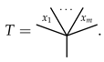
4. Conclusions and Future Studies

Root tree is a good language for constructing free objects. We can intuitively construct algebraic structures through it. In this paper, we mainly construct the free $\mathsf{\Omega }$-Rota–Baxter algebra by typed angularly decorated rooted trees. Further, we hope to provide a more profound characterization from the perspective of operad, representation and homology.

(a)

In 2000, Aguiar established the relationship between Rota–Baxter algebras and Loday’s dendriform algebras. Later, Bai, Guo and Vallete promoted and deepened this connection from the perspective of operad. Operad provides a unified approach to systematically study the relationship between algebraic operations, which helps us to better understand these algebraic structures.

(b)

The Representation theory and homology theory of Rota–Baxter algebras have always been important topics. However, at present, there are just a few articles on the representation of multiple Rota–Baxter algebras, and the theory is still not mature. This leads us to consider the representation theory and homology theory of algebraic structures with a family of operators.

References

1. Baxter, G. An analytic problem whose solution follows from a simple algebraic identity. Pac. J. Math 1960, 10, 731–742. [Google Scholar] [CrossRef]
2. Rota, G.-C. Baxter algebras and combinatorial identities I, II. Bull. Am. Math. Soc. 1969, 75, 325–334. [Google Scholar] [CrossRef] [Green Version]
3. Rota, G.-C. Baxter operators, an introduction. Gian-Carlo Rota on Combinatorics, Introductory Papers and Commentaries. 1995, pp. 504–512. Available online: https://www.amazon.com/Gian-Carlo-Rota-Combinatorics-Introductory-Mathematicians/dp/0817637133 (accessed on 13 November 2021).
4. Cartier, P. On the structure of free Baxter algebras. Adv. Math. 1972, 9, 253–265. [Google Scholar] [CrossRef] [Green Version]
5. Connes, A.; Kreimer, D. Renormalization in quantum field theory and the Riemann-Hilbert problem. I. The Hopf algebra structure of graphs and the main theorem. Commun. Math. Phys. 2000, 210, 249–273. [Google Scholar] [CrossRef] [Green Version]
6. Aguiar, M. Prepoisson algebras. Lett. Math. Phys. 2000, 54, 263–277. [Google Scholar] [CrossRef]
7. Guo, L.; Keigher, W. Baxter algebras and shuffle products. Adv. Math. 2000, 150, 117–149. [Google Scholar] [CrossRef] [Green Version]
8. Guo, L.; Keigher, W. On free Baxter algebras: Completions and the internal construction. Adv. Math. 2000, 151, 101–127. [Google Scholar] [CrossRef] [Green Version]
9. Guo, L.; Zhang, B. Polylogarithms and multiple zeta values from free Rota-Baxter algebras. Sci. China Math. 2010, 53, 2239–2258. [Google Scholar] [CrossRef] [Green Version]
10. Guo, L.; Lang, H.L.; Sheng, Y.H. Integration and geometrization of Rota-Baxter Lie algebras. Adv. Math. 2021, 387, 107834. [Google Scholar] [CrossRef]
11. Zhang, T.; Gao, X.; Guo, L. Hopf algebras of rooted forests, cocyles, and free Rota-Baxter algebras. J. Math. Phys. 2016, 57, 101701. [Google Scholar] [CrossRef] [Green Version]
12. Zheng, H.H.; Guo, L.; Zhang, L.Y. Rota-Baxter paired modules and their constructions from Hopf algebras. J. Algebra 2020, 559, 601–624. [Google Scholar] [CrossRef]
13. Pei, J.; Bai, C.; Guo, L. Splitting of operads and Rota-Baxter operators on operads. Appl. Categ. Struct. 2017, 25, 505–538. [Google Scholar] [CrossRef]
14. Bai, C.; Guo, L.; Ni, X. Generalizations of the classical Yang-Baxter equation and O-operators. J. Math. Phys. 2011, 52, 063515. [Google Scholar] [CrossRef] [Green Version]
15. Bai, C.; Guo, L.; Ni, X. O-operators on associative algebras and associative Yang-Baxter equations. Pacifica J. Math. 2012, 256, 257–289. [Google Scholar] [CrossRef] [Green Version]
16. Bardakov, V.G.; Gubarev, V. Rota-Baxter groups, skew left braces, and the Yang-Baxter equation. arXiv 2021, arXiv:2105.00428. [Google Scholar] [CrossRef]
17. Smoktunowicz, A.; Vendramin, L. On skew braces (with an appendix by N. Byott and L. Vendramin). J. Comb. Algebra 2018, 2, 47–86. [Google Scholar] [CrossRef] [Green Version]
18. Bai, C.; Gao, X.; Guo, L.; Zhang, Y. Operator forms of nonhomogeneous associative classical Yang-Baxter equation. arXiv 2020, arXiv:2007.10939. [Google Scholar]
19. Chen, D.; Luo, Y.F.; Zhang, Y.; Zhang, Y.Y. Free Ω-Rota-Baxter algebras and Gröbner-Shirshov bases. Int. J. Algebra Comput. 2020, 30, 1359–1373. [Google Scholar] [CrossRef]
20. Kurosh, A.G. Free sums of multiple operators algebras. Sib. Math. J. 1960, 1, 62–70. [Google Scholar]
21. Guo, L. Operated monoids, Motzkin paths and rooted trees. J. Algebr. Comb. 2009, 29, 35–62. [Google Scholar] [CrossRef] [Green Version]
22. Foissy, L. Algebraic structures on typed decorated planar rooted trees. SIGMA 2021, 17, 86. [Google Scholar]
23. Foissy, L. Typed binary trees and generalized dendrifom algebras. J. Algebra 2021, 586, 1–61. [Google Scholar] [CrossRef]
24. Zhang, Y.; Gao, X.; Guo, L. Matching Rota-Baxter algebras, matching dendriform algebras and matching pre-Lie algebras. J. Algebra 2020, 552, 134–170. [Google Scholar] [CrossRef] [Green Version]
25. Zhang, Y.Y.; Gao, X. Free Rota-Baxter family algebras and (tri)dendriform family algebras. Pac. J. Math. 2019, 301, 741–766. [Google Scholar] [CrossRef]
26. Zhang, Y.Y.; Gao, X.; Manchon, D. Free Rota-Baxter family algebras and free (tri)dendriform family algebras. arXiv 2020, arXiv:2002.04448v4. [Google Scholar] [CrossRef]
27. Aguiar, M. Dendriform algebras relative to a semigroup. Symmetry Integr. Geom. Methods Appl. 2020, 16, 15. [Google Scholar] [CrossRef]
28. Ma, T.; Li, J. Rota-Baxter Hopf π-(co)algebras. arXiv 2021, arXiv:2104.05529. [Google Scholar]
29. Cayley, A. On the theory of the analytical forms called trees. Philos. Mag. 1857, 13, 172–176. [Google Scholar] [CrossRef]
30. Brouder, C. Runge-Kutta methods and renormalization. Eur. Phys. J. C 2000, 12, 521–534. [Google Scholar] [CrossRef] [Green Version]
31. Connes, A.; Kreimer, D. Hopf algebras, renormalization and non-commutative geometry. Commun. Math. Phys. 1998, 199, 203–242. [Google Scholar] [CrossRef] [Green Version]
32. Chapoton, F.; Livernet, M. Pre-Lie algebras and rooted trees operad. Int. Math. Res. Not. 2001, 8, 396–408. [Google Scholar]
33. Bruned, Y.; Hairer, M.; Zambotti, L. Algebraic renormalisation of regularity structures. Invent. Math. 2019, 215, 1039–1156. [Google Scholar] [CrossRef] [Green Version]
34. Ebrahimi-Fard, K.; Gracia-Bondía, J.M.; Patras, F. A Lie theoretic approach to renormalization. Commun. Math. Phys. 2007, 276, 519–549. [Google Scholar] [CrossRef] [Green Version]
35. Zhang, Y.Y.; Gao, X.; Manchon, D. Free (tri)dendriform family algebras. J. Algebra 2020, 547, 456–493. [Google Scholar] [CrossRef] [Green Version]
36. Guo, L. An Introduction to Rota-Baxter Algebra; International Press: Vienna, Austria, 2012. [Google Scholar]
37. Stanley, R.P. Enumerative Combinatorics, Volume 2: Number 62 in Cambridge Studies in Advanced Mathematics; Cambridge University Press: Cambridge, UK, 1999. [Google Scholar]
Publisher’s Note: MDPI stays neutral with regard to jurisdictional claims in published maps and institutional affiliations.