Automatic Control for Time Delay Markov Jump Systems under Polytopic Uncertainties

Abstract

The Markov jump systems (MJSs) are a special case of parametric switching system. However, we know that time delay inevitably exists in many practical systems, and is known as the main source of efficiency reduction, and even instability. In this paper, the stochastic stable control design is discussed for time delay MJSs. In this regard, first, the problem of modeling of MJSs and their stability analysis using Lyapunov-Krasovsky functions is studied. Then, a state-feedback controller (SFC) is designed and its stability is proved on the basis of the Lyapunov theorem and linear matrix inequalities (LMIs), in the presence of polytopic uncertainties and time delays. Finally, by various simulations, the accuracy and efficiency of the proposed methods for robust stabilization of MJSs are demonstrated.

1. Introduction

Markov Jump Systems (MJS) are a class of parametric switching systems (SSs). The MJSs are represented as a set of systems that are constantly in transition between models with a Markov process with a limited state number. These systems can also be classified as a case of hybrid SSs, in which switchings are managed by a Markov chain the Ref. [1]. Mathematically, Markov jump systems are classified as random systems, in which the system matrices are randomly jumped at a series of discrete times managed by the Markov process, and in the time between these random jumps, these matrices are time-invariant. Due to their widespread use in practical systems, significant attention has been paid to them in the last few decades. These systems are used to model a variety of processes, including sudden changes in structures, such as accidental breakdowns and sudden disturbances, environmental changes, and changes in the internal connections of subsystems, power systems and solar panels, flight controllers, modeling abrupt changes in economic systems and modeling and predicting network control systems. Many researchers have addressed the problem of modeling Markov jump systems, analyzing their stability and efficiency, designing a variety of controllers, including state feedback [2], robust H${}_{\infty }$ [3], output feedback [4], and sliding mode control [5].

MJSs were first introduced by Krasovsky and Lidsky in 1961, who studied the control process of a system subject to stochastic changes and expressed the style of this class of systems [6]. Vanham was then one of the pioneering researchers in the development of these systems, developing mathematical models and algorithms suitable for complex dynamic systems, which are under natural constraints and random perturbations [7]. In the model of economics studied in the Refs. [8,9], it is considered that the state of the economy can be described as one of three functional modes: “normal”, “rapid growth”, or “recession”. Additionally, switching between these states can be modeled as a Markov-chain. In 1983, Aswarder et al. developed Markovian jump systems based on optimal control and random estimation [10]. Since then, the stability study of MJSs has been increased significantly. This is due to the fact that most practical systems are inherently exposed to stochastic changes and sudden environmental disturbances. Markov jump systems are also used to analyze the stability of controlled flight systems, which operates under various perturbations [11,12].

The Markov jumps are used in the control and dynamic identification of power systems [13], in which a switching mechanism is used to identify sudden load changes, production unit disconnection, and transmission line defects. The security criterion that is used to determine the vulnerability of the current state of the system and network topology can also be represented by a finite-time Markov process and a model-dependent jump. In network control systems, data latency and loss are the two main phenomena that occur due to the existence of the network, which must be considered in the design of the controller; otherwise, the efficiency drops sharply. One of the methods of modeling these two phenomena is as an MJS system [14].

2. Literature Review

In the Ref. [15], the H${}_{\infty }$ controller developed MJSs, and the improvement of the transient behavior was studied. In the Ref. [16], the feedback controller was formulated, and the time delay effect was investigated. The passivity analysis was presented in the Ref. [17], and the effect of deception attacks was studied by designing an asynchronous control scenario. In the Ref. [18], the application of the theory of MJSs in robotic problems was addressed, and the control scheme was developed for disturbance rejection. A quantized control scheme was designed in the Ref. [19] for Roesser MJS, and the feasibility of a designed controller in some applications was investigated. In the Ref. [20], by the use of neural networks (NN), the nonlinear dynamics in MJSs were eliminated, and the system dynamics were converted to the linear sub-systems, and then an optimal controller was designed for linearized models. The self-triggered scheme was developed in the Ref. [21], and by designing an H${}_{\infty }$-based control system, the signal boundedness was ensured. The fuzzy controllers were investigated in the Ref. [22], and the problem of stochastic stability was analyzed.

The nonlinear MJSs under time delay has been rarely studied. For example, in the Ref. [23], the exponential stability was analyzed under time delay, and some stability conditions were derived via a LMI approach. The event-triggered scheme was studied in the Ref. [24], and a H${}_{\infty }$-based controller was designed for fuzzy MJSs. The time-varying delay problem was addressed in the Ref. [25], and the output boundedness was ensured by the suggested LMI technique. In the Ref. [26], the time delay was studied by the use of fuzzy rules, and by the Lyapunov-Krasovskii approach, some stability conditions were suggested. In the Ref. [27], the discrete-time MJSs were taken into account, and the stochastic stability was proven. In this paper, some conditions were extracted to guarantee stability against time delay. The L1-gain analysis was developed in the Ref. [28] for MJS, and the stability against time delays was investigated. In the Ref. [29], the $L_{\infty }$ scheme was developed for fuzzy MJSs, and the effect of transmission delay was studied. In the Refs. [30,31,32,33,34], the various versions of a sliding-mode controller (SMC), such as a simple SMC, integral SMC, backstepping SMC, and terminal were studied, and they were applied on an under-actuated quadcopter.

3. Novelties

The literature review shows that the state-feedback control system has been designed for the delayed MJSs. However, in most of them, the system equations are considered nominally, or structural uncertainties such as $\Delta A=EF\left(t\right)H$ are used in control design, in which $\Delta A$ is a real function, E and H are known matrices, and unknown $F\left(t\right)$ satisfies $F{\left(t\right)}^{T}F\left(t\right)\le I$. According to the literature review, in very few studies, the control design for MJSs under polytopic uncertainties was discussed. The main difficulties are the effect of polytopic uncertainties, time delays, and restrictions on LMI sets. The basic novelties are:

• Introducing a suitable Lyapunov-Krasovsky function to analyze the stability of the time delayed MJSs, and extract a sufficient condition in the LMI form to find a higher delay bound;
• Analyzing the stability of the MJSs in the presence of polytopic uncertainty and generalizing the obtained results; and
• Designing the controller using a mode-dependent state feedback approach and finding appropriate control gains in LMI form.

4. Problem Description

We consider the dynamical model of a MJS as [35]:

$$\begin{array}{c}\hfill \left\{\begin{array}{cc}\hfill & \dot{\chi }\left(t\right)=\mathcal{A}\left(r_t\right)\chi \left(t\right)+{\mathcal{A}}_d\left(r_t\right)\chi (t-\tau )+\mathcal{B}\left(r_t\right)u\left(t\right)\hfill \\ \hfill & y\left(t\right)=\mathcal{C}\left(r_t\right)\chi \left(t\right)\hfill \\ \hfill & \chi \left(t\right)=\mathsf{\Phi }\left(t\right)r\left(0\right)=r_{0}t\in [-\tau ,0],\hfill \end{array}\right.\end{array}$$

(1)

where $\chi \left(t\right)\in {\mathbb{R}}^n/u\left(t\right)\in {\mathbb{R}}^m$, and $y\left(t\right)\in {\mathbb{R}}^l$ are the continuous-time state/controller and output, respectively; $\tau >0$ represents the constant delay; $\left\{r_t\right\}$ is a homogeneous finite-state Markov process; $\mathcal{A}\left(r_t\right),{\mathcal{A}}_d\left(r_t\right)\in {\mathbb{R}}^{n\times n},\mathcal{B}\left(r_t\right)\in {\mathbb{R}}^{n\times m},$ and $\mathcal{C}\left(r_t\right)\in {\mathbb{R}}^{l\times n}$. The initial state of the system is indicated as $\left(r_0,\mathsf{\Phi }(.)\right)$ with $\chi \left(\vartheta \right)=\mathsf{\Phi }\left(\vartheta \right)\in L_2[-\tau ,0]$ and ${\chi }_0=\mathsf{\Phi }\left(0\right)$.

Contemplate a system with modes, $S=\{1,2,\dots ,N\}$ and infinitesimal generator $\Lambda =\left({\lambda }_{i,j}\right),i,j\in S$, where $\Lambda ={\lambda }_{i,j}\ge 0,\forall j\ne i,{\lambda }_{i,i}=-{\sum }_{j\ne i}{\lambda }_{i,j}$. Then, the transition probabilities are given as [36]:

$$\begin{array}{c}\hfill P[r_{t+\Delta }=j|r_t=i]=\left\{\begin{array}{cc}{\lambda }_{i,j}\Delta +o(\Delta ),\hfill & j\ne i\hfill \\ 1+{\lambda }_{i,j}\Delta +o(\Delta ),\hfill & j=i.\hfill \end{array}\right.\mathrm{where}\underset{\Delta \to 0}{lim}\frac{o(\Delta )}{\Delta }=0.\end{array}$$

(2)

5. Preliminaries

Definition 1.

The polytopic-type uncertainties are defined as follows

$$\begin{array}{c}\hfill {\Lambda }_i=\left\{\left[{\mathcal{A}}_i{\mathcal{A}}_{di}{\mathcal{B}}_i\right]|\left[{\mathcal{A}}_i{\mathcal{A}}_{di}{\mathcal{B}}_i\right]=\sum _{r=1}^{{\nu }_i}{\beta }_{ir}\left[{\mathcal{A}}_{ir}{\mathcal{A}}_{dir}{\mathcal{B}}_{ir}\right];{\beta }_{ir}\ge 0,\sum _{r=1}^{{\nu }_i}{\beta }_{ir}=1\right\},\end{array}$$

(3)

where ${\nu }_i$ denotes the number of the vertices of ${\Lambda }_i$, ${\beta }_{ir}(r=1,\dots ,{\nu }_i)$ are the time-invariant uncertainties, ${\mathcal{A}}_{ir},{\mathcal{A}}_{dir}$ and ${\mathcal{B}}_{ir}$ are known matrices and ${\mathcal{A}}_i,{\mathcal{A}}_{di}$ and ${\mathcal{B}}_i,$ are unknown matrices.

Definition 2.

For the finite $\mathsf{\Phi }\left(t\right)\in {\mathbb{R}}^n$ and all initial modes $r_0\in S$, the stochastic stability of MJS is ensured if the following inequality exists:

$$\begin{array}{c}\hfill \underset{t\to \infty }{lim}E\left\{{\int }_0^t{\chi }^T(q,\mathsf{\Phi },r_0)\chi (q,\mathsf{\Phi },r_0)dq\right\}<\infty ,\end{array}$$

(4)

where $u\left(t\right)=0$, $\chi (q,\mathsf{\Phi },r_0)$ represents a solution, and Φ and $r_0$ are initial conditions.

Definition 3.

The weak infinitesimal generator of a stochastic process ($\mathcal{J}$) is written as:

$$\begin{array}{c}\mathcal{J}V\left(\chi \right(t),i,t)=\hfill \\ \underset{\Delta \to 0}{lim}\frac{1}{\Delta }\left\{\begin{array}{c}E\left[V\left(\chi \right(t+\Delta ),r(t+\Delta ),t+\Delta )\left|\chi \right(t),r(t)=i\right]\hfill \\ -V\left(\chi \left(t\right),i,t\right)\hfill \end{array}\right\}\hfill \end{array}$$

(5)

Lemma 1.

Finsler’s Lemma: Consider real matrices $\Omega \in {\mathbb{R}}^{n\times n}$ and the full row rank matrix $F\in {\mathbb{R}}^{m\times n}$, then we can write:

• For $\xi \in {\mathbb{R}}^n$, we can write ${\xi }^T\left(t\right)\Omega \xi \left(t\right)<0$ and $F\xi \left(t\right)=0$;
• For a scalar $\mu \in \mathbb{R}$ we can write $\mu +F^{T}F<0$;
• The following condition holds: $F^{\perp T}\Omega F^{\perp }<0$

Lemma 2.

Consider matrices $W,U,V,T_1,T_2$ and suppose that $T_1>0,T_2>0,$ and that U/V have column/row full ranks. Then there exists a matrix Σ such that:

$$\left(W+U\Sigma V\right)T_1{\left(W+U\Sigma V\right)}^T-T_2<0$$

(6)

if, and only if:

$$\begin{array}{cc}\hfill U^{\perp }\left(T_2-W{T}_1{W}^T\right)U^{\perp T}& >0\hfill \\ \hfill V^{T\perp }\left(T_1^{-1}-W{T}_2^{-1}W\right)V^{T\perp T}& >0.\hfill \end{array}$$

(7)

Theorem 1.

The stability of MJS (1) with $u\left(t\right)=0$ is ensured for any time delay $\tau >0$, if we have $P_i>0,Q>0,Z>0$ such that the:

$$\begin{array}{c}\hfill {\Omega }_i=F_i^{\perp T}\left[{\Theta }_i+{\overline{P}}_i\right]F_i^{\perp }<0\end{array}$$

(8)

where, $i=1,2,\dots ,N$, and

$$\begin{array}{cccc}\hfill F_i& =\left[\begin{array}{cccc}{\mathcal{A}}_i& {\mathcal{A}}_{di}& 0& -I\\ I& -I& -I& 0\end{array}\right]\hfill & \hfill P^i=& \sum _{j=1}^N{\lambda }_{ij}{P}_j\hfill \\ \hfill {\Theta }_i& =\left[\begin{array}{cccc}Q& 0& 0& P_i\\ & -Q& 0& 0\\ & *& -Z& 0\\ & *& *& {\iota }^{2}Z\end{array}\right]\hfill & \hfill {\overline{P}}^i=& \mathrm{diag}\{P^i,0,0,0\}.\hfill \end{array}$$

Note that $F_i^{\perp T}$ denotes the orthogonality complement of $F_i$ and ${\Theta }_i\left(\iota \right)={\Theta }_i$ is defined.

Proof. 

The stochastic Lyapunov-Krasovskii functional is considered as

$$\begin{array}{cc}\hfill V\left(\chi \right(t),r(t\left)\right)& ={\chi }^T\left(t\right)P_i\chi \left(t\right)+{\int }_{t-\iota }^t{\chi }^T\left(\vartheta \right)Q\chi \left(\vartheta \right)\mathrm{d}\#\hfill \\ \hfill & +\iota {\int }_{-\iota }^0{\int }_{t+\theta }^t{\dot{\chi }}^T\left(\vartheta \right)Z\dot{\chi }\left(\vartheta \right)\mathrm{d}\#\mathrm{d}‘,\hfill \end{array}$$

(9)

where $P_i=P\left(r\left(t\right)\right)$ when $r\left(t\right)=i$. Consider $\mathcal{J}$ for process $\{{\chi }_t,r_t\}$, then, for each $r_t=i(i\in S)$, we have:

$$\begin{array}{cc}\hfill & V_1(\chi \left(t\right),r\left(t\right))={\chi }^T\left(t\right)P_i\chi \left(t\right)\to \hfill \\ \hfill & \mathcal{J}{V}_1(\chi \left(t\right),r\left(t\right))=\underset{\Delta \to 0^{+}}{lim}\frac{1}{\Delta }\left\{E\left[{\chi }^T(t+\Delta )P_{r(t+\Delta )}\chi (t+\Delta )\right]-{\chi }^T\left(t\right)P_i\chi \left(t\right)\right\}\hfill \\ \hfill & =\underset{\Delta \to 0^{+}}{lim}\frac{1}{\Delta }\left\{E\left[{\left(\Delta \dot{\chi }\left(t\right)+\chi \left(t\right)\right)}^T{P}_{r(t+\Delta )}\left(\Delta \dot{\chi }\left(t\right)+\chi \left(t\right)\right)\right]-{\chi }^T\left(t\right)P_i\chi \left(t\right)\right\}\hfill \\ \hfill & =\underset{\Delta \to 0^{+}}{lim}\frac{1}{\Delta }\left\{E\left[{\Delta }^2{\dot{\chi }}^T\left(t\right)P_{r(t+\Delta )}\dot{\chi }\left(t\right)\right]+E\left[\Delta \left({\chi }^T\left(t\right)P_{r(t+\Delta )}\dot{\chi }\left(t\right)+{\dot{\chi }}^T\left(t\right)P_{r(t+\Delta )}\chi \left(t\right)\right)\right]\right.\hfill \\ \hfill & \left.+E\left[{\chi }^T\left(t\right)P_{r(t+\Delta )}\chi \left(t\right)\right]-{\chi }^T\left(t\right)P_i\chi \left(t\right)\right\}\hfill \\ \hfill & =0+\left({\chi }^T\left(t\right)P_{r\left(t\right)}\dot{\chi }\left(t\right)+{\dot{\chi }}^T\left(t\right)P_{r\left(t\right)}\chi \left(t\right)\right)+\underset{\Delta \to 0^{+}}{lim}\frac{1}{\Delta }\left({\chi }^T\left(t\right)\left(\sum _{j=1,j\ne i}^N{\lambda }_{ij}\Delta P_j+{\lambda }_{ii}\Delta P_i\right)\chi \left(t\right)\right)\hfill \end{array}$$

$$\begin{array}{cc}\hfill & +{\chi }^T\left(t\right)P_i\dot{\chi }\left(t\right)+{\dot{\chi }}^T\left(t\right)P_i\chi \left(t\right)+{\chi }^T\left(t\right)\left(\sum _{j=1}^N{\lambda }_{ij}{P}_j\right)\chi \left(t\right)\hfill \\ \hfill & V_2(\chi \left(t\right),r\left(t\right))={\int }_{t-\iota }^t{\chi }^T\left(\vartheta \right)Q\chi \left(\vartheta \right)\mathrm{d}\#\to \hfill \\ \hfill & \mathcal{J}{V}_2(\chi \left(t\right),r\left(t\right))=\underset{\Delta \to 0^{+}}{lim}\frac{1}{\Delta }\left(E\left[{\int }_{t+\Delta -\iota }^{t+\Delta }{\chi }^T\left(\vartheta \right)Q\chi \left(\vartheta \right)\mathrm{d}\#\right]-{\int }_{t-\iota }^t{\chi }^T\left(\vartheta \right)Q\chi \left(\vartheta \right)\mathrm{d}\#\right)\hfill \\ \hfill & \underset{\Delta \to 0^{+}}{lim}\frac{1}{\Delta }\left({\int }_t^{t+\Delta }{\chi }^T\left(\vartheta \right)Q\chi \left(\vartheta \right)\mathrm{d}\#-{\int }_{\mathrm{t}-´}^{\mathrm{t}-´+■}{\chi }^{\mathrm{T}}\left(\#\right)\mathrm{Q}\chi \left(\#\right)\mathrm{d}\#\right)\hfill \\ \hfill & \underset{\Delta \to 0^{+}}{lim}\frac{1}{\Delta }\left(\Delta {\chi }^T\left(t\right)Q\chi \left(t\right)-\Delta {\chi }^T(t-\iota )Q\chi (t-\iota )\right)\hfill \end{array}$$

(10)

$$\begin{array}{cc}\hfill & ={\chi }^T\left(t\right)Q\chi \left(t\right)-{\chi }^T(t-\iota )Q\chi (t-\iota )\hfill \\ \hfill & V_3(\chi \left(t\right),r\left(t\right))=\iota {\int }_{-\iota }^0{\int }_{t+\theta }^t{\dot{\chi }}^T\left(\vartheta \right)Z\dot{\chi }\left(\vartheta \right)\mathrm{d}\#\mathrm{d}‘\to \hfill \\ \hfill & \mathcal{J}{V}_3(\chi \left(t\right),r\left(t\right))=\iota \underset{\Delta \to 0^{+}}{lim}\frac{1}{\Delta }\left(E\left[{\int }_{-\iota }^0{\int }_{t+\theta +\Delta }^{t+\Delta }{\dot{\chi }}^T\left(\vartheta \right)Z\dot{\chi }\left(\vartheta \right)\mathrm{d}\#\mathrm{d}‘\right]-{\int }_{-‘}^0{\int }_{t+■+‘}^{t+‘}{\dot{\chi }}^T\left(\#\right)Z\dot{\chi }\left(\#\right)\mathrm{d}\#\mathrm{d}‘\right)\hfill \\ \hfill & =\iota \underset{\Delta \to 0^{+}}{lim}\frac{1}{\Delta }\left({\int }_{-\iota }^0{\int }_t^{t+\Delta }{\dot{\chi }}^T\left(\vartheta \right)Z\dot{\chi }\left(\vartheta \right)\mathrm{d}\#\mathrm{d}‘-{\int }_{-´}^0{\int }_{\mathrm{t}+‘}^{\mathrm{t}+■+‘}{\dot{\chi }}^{\mathrm{T}}\left(\#\right)\mathrm{Z}\dot{\chi }\left(\#\right)\mathrm{d}\#\mathrm{d}‘\right)\hfill \\ \hfill & \iota {\int }_{-\iota }^0{\dot{\chi }}^T\left(\vartheta \right)Z\dot{\chi }\left(\vartheta \right)d\theta -\iota {\int }_{-\iota }^0{\dot{\chi }}^T(t+\theta )Z\dot{\chi }(t+\theta )d\theta \hfill \end{array}$$

(11)

$$\begin{array}{cc}\hfill & ={\iota }^2{\dot{\chi }}^T\left(t\right)Z\dot{\chi }\left(t\right)-\iota {\int }_{t-\iota }^t{\dot{\chi }}^T\left(\vartheta \right)Z\dot{\chi }\left(\vartheta \right)d\vartheta .\hfill \end{array}$$

(12)

From Jensen’s inequality, one has

$$\begin{array}{c}\hfill -\iota {\int }_{t-\iota }^t{\dot{\chi }}^T\left(\vartheta \right)Z\dot{\chi }\left(\vartheta \right)d\vartheta \le -{\left({\int }_{t-\iota }^t{\dot{\chi }}^T\left(\vartheta \right)d\vartheta \right)}^{T}Z\left({\int }_{t-\iota }^t\dot{\chi }\left(\vartheta \right)d\vartheta \right)\end{array}$$

(13)

Thus

$$\begin{array}{cc}\hfill & \mathcal{J}V(\chi \left(t\right),r\left(t\right))=\mathcal{J}{V}_1(\chi \left(t\right),r\left(t\right))+\mathcal{J}{V}_2(\chi \left(t\right),r\left(t\right))+\mathcal{J}{V}_3(\chi \left(t\right),r\left(t\right))\hfill \\ \hfill & =+{\chi }^T\left(t\right)P_i\dot{\chi }\left(t\right)+{\dot{\chi }}^T\left(t\right)P_i\chi \left(t\right)+{\chi }^T\left(t\right)\left(\sum _{j=1}^N{\lambda }_{ij}{P}_j\right)\chi \left(t\right)\hfill \\ \hfill & +{\chi }^T\left(t\right)Q\chi \left(t\right)-{\chi }^T(t-\iota )Q\chi (t-\iota )\hfill \\ \hfill & +{\iota }^2{\dot{\chi }}^T\left(t\right)Z\dot{\chi }\left(t\right)-{\left(\chi \left(t\right)-\chi (t-\iota )\right)}^{T}Z\left(\chi \left(t\right)-\chi (t-\iota )\right)\hfill \end{array}$$

(14)

Considering

$$\begin{array}{c}\hfill \xi \left(t\right)={\left[\begin{array}{cccc}{\chi }^T\left(t\right)& {\chi }^T(t-\iota )& {\left({\int }_{t-\iota }^t\dot{\chi }\left(\vartheta \right)d\vartheta \right)}^T& {\dot{\chi }}^T\left(t\right)\end{array}\right]}^T\end{array}$$

(15)

One can achieve

$$\begin{array}{c}\hfill \mathcal{J}V(\chi \left(t\right),r\left(t\right))={\xi }^T\left(t\right)\left[{\Theta }_i+{\overline{P}}_i\right]\xi \left(t\right).\end{array}$$

(16)

Therefore it is obvious that $\mathcal{J}V\left(\chi \right(t),r(t\left)\right)<0$ holds if:

$$\begin{array}{c}\hfill {\xi }^T\left(t\right)\left[{\Theta }_i+{\overline{P}}_i\right]\xi \left(t\right)<0.\end{array}$$

(17)

Regarding the Newton-Leibniz formula, one has

$$\begin{array}{cc}\hfill & {\int }_{t-\iota }^t\dot{\chi }\left(\vartheta \right)d\vartheta =\chi \left(t\right)-\chi (t-\iota )\to \chi \left(t\right)-\chi (t-\iota )-{\int }_{t-\iota }^t\dot{\chi }\left(\vartheta \right)d\vartheta =0\hfill \end{array}$$

(18)

$$\begin{array}{cc}\hfill & -\dot{\chi }\left(t\right)+\mathcal{A}\left(r_t\right)\chi \left(t\right)+{\mathcal{A}}_d\left(r_t\right)\chi (t-\iota )=0,\hfill \end{array}$$

(19)

or equivalently,

$$\begin{array}{c}\hfill \left[\begin{array}{cccc}{\mathcal{A}}_i& {\mathcal{A}}_{di}& 0& -I\\ I& -I& -I& 0\end{array}\right]\xi \left(t\right)=0\to F_i\xi \left(t\right)=0.\end{array}$$

(20)

The equalities (21) and (18) hold, if and only if:

$$\begin{array}{c}\hfill F_i^{\perp T}\left[{\Theta }_i+{\overline{P}}_i\right]F_i^{\perp }<0i=1,2,\dots ,N.\end{array}$$

(21)

This completes the proof. □

6. Main Results

Theorem 2.

The stochastic stability of MJS (1) is ensured for time delay ι, if for ${\Psi }_i,P_i>0,Q>0,Z>0$ and scalars ${\mu }_i>0$, we have:

$$\begin{array}{c}\hfill S\triangleq \left[\begin{array}{cc}{\Theta }_i+{\overline{P}}_i-{\mu }_{i}I& {\mu }_{i}I+F_i^T{\Psi }_i\\ & -{\mu }_{i}I\end{array}\right]<0\end{array}$$

(22)

where $u\left(t\right)=0$, $i=1,2,\dots ,N$.

Proof. 

According to Lemma 2, define $T_{1i}={\mu }_{i}I\in {\mathbb{R}}^{4n\times 4n}$ with enough large scalars ${\mu }_i>0,T_{2i}=T_{1i}-\left({\Theta }_i+{\overline{P}}_i\right)>0,U_i=F_i^T,V_i=I,W_i=I$. Now, if there exist ${\Sigma }_i\in {\mathbb{R}}^{2n\times 4n}$, with full row ranks, such that:

$$\begin{array}{c}\hfill {\mu }_i\left(I+F_i^T{\Sigma }_i\right){\left(I+F_i^T{\Sigma }_i\right)}^T+{\Theta }_i+{\overline{P}}_i-{\mu }_{i}I<0.\end{array}$$

(23)

Then, the LMIs (23) hold by using the change of variable ${\Psi }_i={\mu }_i{\Sigma }_i$. Moreover, it is evident by the system (1) by $\left(u\left(t\right)=0\right)$ that in the presence of time delays it is stochastically stable, and this completes the proof. □

Remark 1.

Before expressing the next Theorem, since LMIs (23) are affine in respect of ${\mathcal{A}}_i$ and ${\mathcal{A}}_i$, sufficient conditions for investigating the robust stochastic stability in the presence of polytopic uncertainties can be acquired by considering the proposed LMIs only in polytopic uncertainty vertices for each mode. In other words, the corresponding system subject to polytopic uncertainties has robust stochastic stability if the following LMIs have feasible solutions:

$$\begin{array}{c}\hfill S\triangleq \left[\begin{array}{cc}{\Theta }_i+{\overline{P}}_i-{\mu }_{i}I& {\mu }_{i}I+F_{ir}^T{\Psi }_i\\ & -{\mu }_{i}I\end{array}\right]<0i=1,2,\dots ,N,r=1,2,\dots ,{\nu }_i\end{array}$$

(24)

where:

$$\begin{array}{c}\hfill F_{ir}=\left[\begin{array}{cccc}{\mathcal{A}}_{ir}& {\mathcal{A}}_{dir}& 0& -I\\ I& -I& -I& 0\end{array}\right]\end{array}$$

Proof.

For each i, we multiply inequalities of (25) by scalars ${\beta }_{ir},r=1,\dots ,N$, where ${\sum }_{r=1}^{{\nu }_i}{\beta }_{ir}=1,{\beta }_{ir}>0$ and we sum up the achieved results with each other, and the LMIs of (23) are extracted. □

Since Lyapunov matrices $(P_i,Q,Z)$ of LMIs (25) are independent of the system matrices, the suggested results are conservative. Therefore, the next Theorem will be proposed to reduce the conservatism of the robust stability analysis of the MJS. In this regard, the following matrices are defined

$$\begin{array}{c}\hfill :P_i\left({\beta }_i\right)=\sum _{r=1}^{{\nu }_i}{\beta }_{ir}{P}_i^{\left(r\right)}\end{array}$$

$$\begin{array}{c}\hfill Q_i\left({\beta }_i\right)=\sum _{r=1}^{{\nu }_i}{\beta }_{ir}{Q}^{\left(r\right)}\end{array}$$

(25)

$$\begin{array}{c}\hfill Z_i\left({\beta }_i\right)=\sum _{r=1}^{{\nu }_i}{\beta }_{ir}{Z}^{\left(r\right)}i=1,\dots ,N\end{array}$$

(26)

where $P_i^{\left(r\right)},Q^{\left(r\right)},Z^{\left(r\right)}$ are positive definite matrices. Moreover, considering $\mathcal{P}={[P_1\dots P_N]}^T$ and ${\Pi }_i={[{\lambda }_{i1}{I}_n\dots {\lambda }_{iN}{I}_n]}^T$, one has

$$\begin{array}{c}\hfill P^i=\sum _{j=1}^N{\lambda }_{ij}{P}_j={\Pi }_i^T\mathcal{P}.\end{array}$$

(27)

Theorem 3.

Consider MJS (1) with the system matrices belonging to polytopic uncertainty in the form of (3), the system has robust stochastic stability if, for $\iota >0$, there exist matrices ${\Psi }_i,P_i^{\left(r\right)}>0,Q^{\left(r\right)}>0,Z^{\left(r\right)}>0$ and scalars ${\mu }_i^{(}r)>0$, such that:

$$\begin{array}{cc}\hfill & S\triangleq \left[\begin{array}{cc}{\Theta }_i^{\left(r\right)}+{\overline{P}}_i^{\left[{\pi }_{ir}\right]}-{\mu }_i^{\left(r\right)}I& {\mu }_i^{\left(r\right)}I+F_{ir}^T{\Psi }_i\\ & -{\mu }_i^{\left(r\right)}I\end{array}\right]<0\hfill \\ \hfill & i=1,2,\dots ,N,r=1,2,\dots ,{\nu }_i,\forall {\pi }_{ir}\in {\mathcal{I}}_{ir},\hfill \end{array}$$

(28)

where

$$\begin{array}{cc}\hfill & F_{ir}=\left[\begin{array}{cccc}{\mathcal{A}}_{ir}& {\mathcal{A}}_{dir}& 0& -I\\ I& -I& -I& 0\end{array}\right]\hfill \\ \hfill & {\overline{P}}_i^{\left[{\pi }_{ir}\right]}=\mathrm{diag}\left\{{\Pi }_i^T{\mathcal{P}}^{\left[{\pi }_{ir}\right]},0,0,0\right\}\hfill \\ \hfill & {\Theta }_i^{\left(r\right)}=\left[\begin{array}{cccc}{Q}^{\left(r\right)}& 0& 0& P_i^{\left(r\right)}\\ & -Q^{\left(r\right)}& 0& 0\\ & *& -Z^{\left(r\right)}& 0\\ & *& *& {\iota }^2{Z}^{\left(r\right)},\end{array}\right]\hfill \end{array}$$

where ${\mathcal{I}}_{ir}$ indicates the N-tuple sets of the following form:

$$\begin{array}{c}\hfill {\mathcal{I}}_{ir}=\left\{{\pi }_{ir}|{\pi }_{ir}=\left[p_1\dots p_{i-1}r{p}_{i+1}\dots p_N\right],p_{\vartheta }=1,\dots ,{\nu }_{\vartheta },\forall \vartheta \in \left\{1,\dots ,N\right\},\vartheta \ne i\right\}.\end{array}$$

(29)

Hence, for each ${\pi }_{ir}$, there exists the following matrix:

$$\begin{array}{c}\hfill {\mathcal{P}}^{{\pi }_{ir}}=\left[P_1^{p_1}\dots P_{i-1}^{p_{i-1}}{P}_i^r{P}_{i+1}^{p_{i+1}}\dots P_N^{p_N}\right].\end{array}$$

(30)

Proof. 

Considering polytopic uncertainties and multiplying LMIs of Theorem 2 by ${\beta }_{jk},k=1,\dots ,{\nu }_j$ summing them up leads to

$$\begin{array}{cc}\hfill & \sum _{k=1}^{{\nu }_j}{\beta }_{jk}\left[\begin{array}{cc}{\Theta }_i^{\left(r\right)}+{\overline{P}}_i^{\left[{\pi }_{ir}\right]}-{\mu }_i^{\left(r\right)}I& {\mu }_i^{\left(r\right)}I+F_{ir}^T{\Psi }_i\\ & -{\mu }_i^{\left(r\right)}I\end{array}\right]\hfill \\ \hfill & =\left[\begin{array}{cc}{\Theta }_i^{\left(r\right)}+{\overline{P}}_i^{\left[{\Omega }_{ir}\right]}-{\mu }_i^{\left(r\right)}I& {\mu }_i^{\left(r\right)}I+F_{ir}^T{\Psi }_i\\ & -{\mu }_i^{\left(r\right)}I\end{array}\right]<0,\hfill \end{array}$$

(31)

where

$$\begin{array}{cc}\hfill & {\mathcal{P}}^{\left[{\Omega }_{ir}\right]}={\left[P_1\left({\beta }_1\right)\dots P_{i-1}\left({\beta }_{i-1}\right)P_i^{\left(r\right)}{P}_{i+1}\left({\beta }_{i+1}\right)\dots P_N\left({\beta }_N\right)\right]}^T\hfill \\ \hfill & {\overline{P}}_i^{\left[{\Omega }_{ir}\right]}=\mathrm{diag}\left\{{\Pi }_i^T{\mathcal{P}}^{\left[{\Omega }_{ir}\right]},0,0,0\right\}.\hfill \end{array}$$

Now, multiplying (32) by scalars ${\beta }_{ir},r=1,2,\dots ,{\nu }_i$ and summing them up, we conclude:

$$\begin{array}{cc}\hfill & \sum _{k=1}^{{\nu }_i}{\beta }_{ir}\left[\begin{array}{cc}{\Theta }_i^{\left(r\right)}+{\overline{P}}_i^{\left[{\Omega }_{ir}\right]}-{\mu }_i^{\left(r\right)}I& {\mu }_i^{\left(r\right)}I+F_{ir}^T{\Psi }_i\\ & -{\mu }_i^{\left(r\right)}I\end{array}\right]\hfill \\ \hfill & =\left[\begin{array}{cc}{\Theta }_i\left({\beta }_i\right)+{\overline{P}}_i^{\left[{\pi }_{ir}\right]}\left({\beta }_i\right)-{\mu }_i\left({\beta }_i\right)I& {\mu }_i\left({\beta }_i\right)I+F_i^T{\Psi }_i\\ & -{\mu }_{i}I\end{array}\right]<0,\hfill \end{array}$$

(32)

where

$$\begin{array}{cc}\hfill & {\mathcal{P}}^{\left[{\pi }_{ir}\right]}={\left[P_1\left({\beta }_1\right)\dots P_{i-1}\left({\beta }_{i-1}\right)P_i^{\left(r\right)}{P}_{i+1}\left({\beta }_{i+1}\right)\dots P_N\left({\beta }_N\right)\right]}^T\hfill \\ \hfill & {\overline{P}}_i^{\left[{\pi }_{ir}\right]}=\mathrm{diag}\left\{{\Pi }_i^T{\mathcal{P}}^{\left[{\pi }_{ir}\right]}\left({\beta }_i\right),0,0,0\right\}\hfill \end{array}$$

□

State Feedback Controller

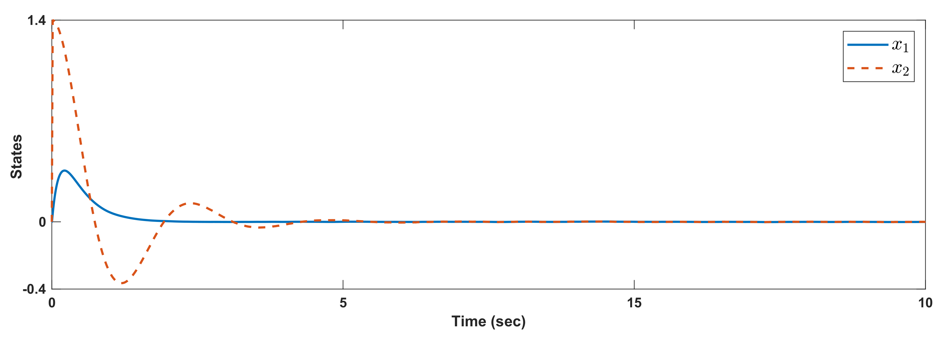
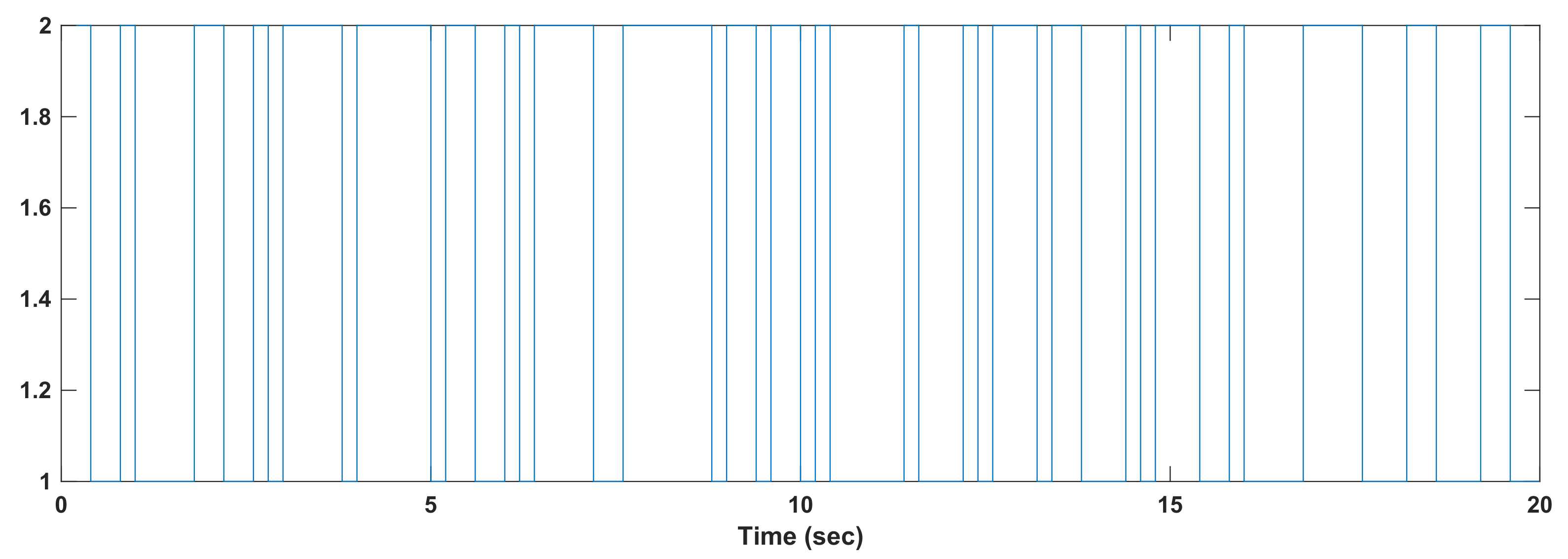
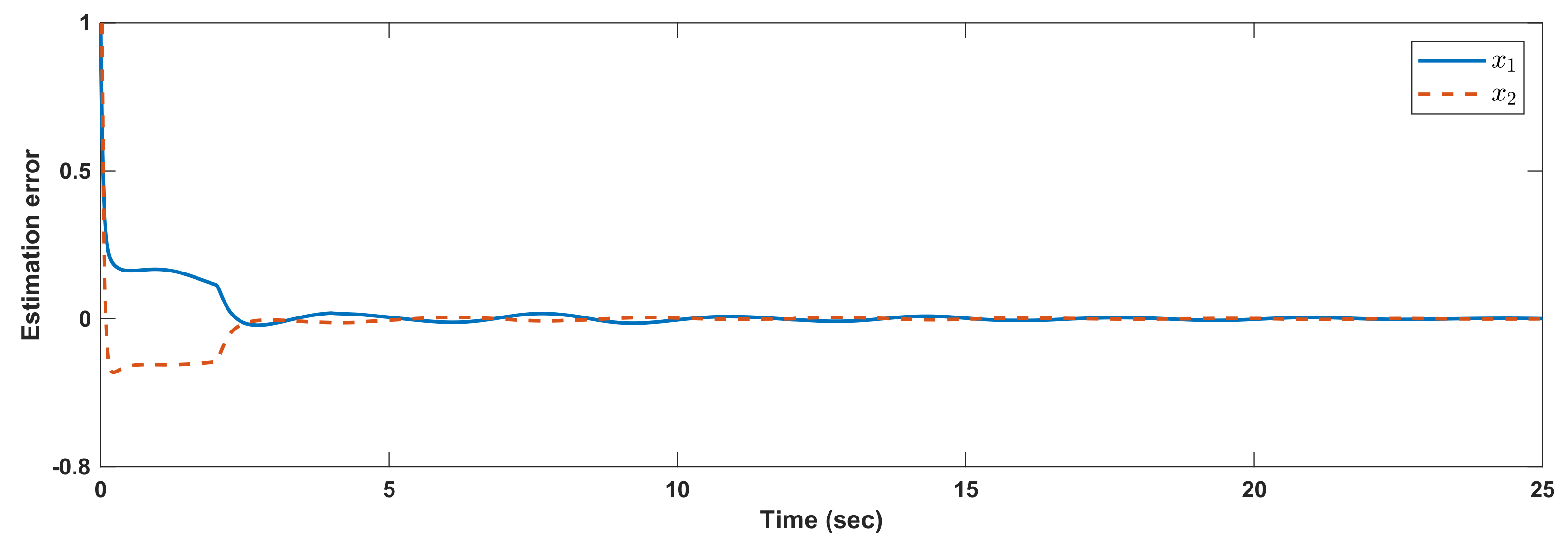
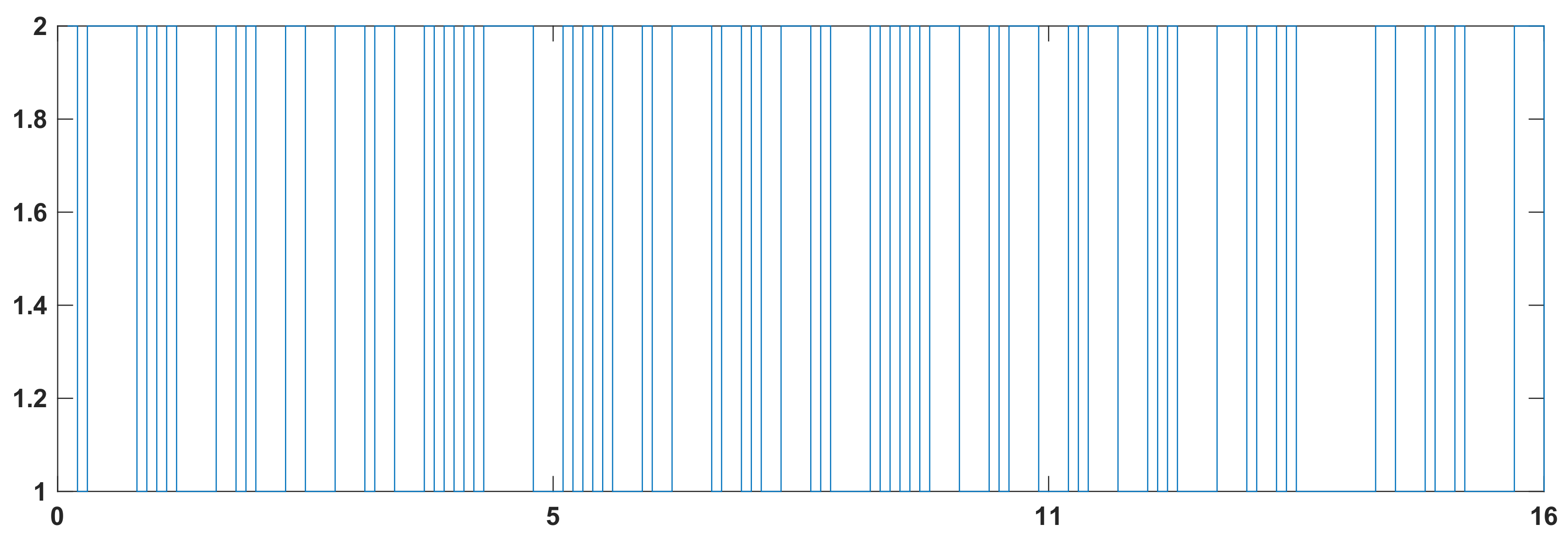
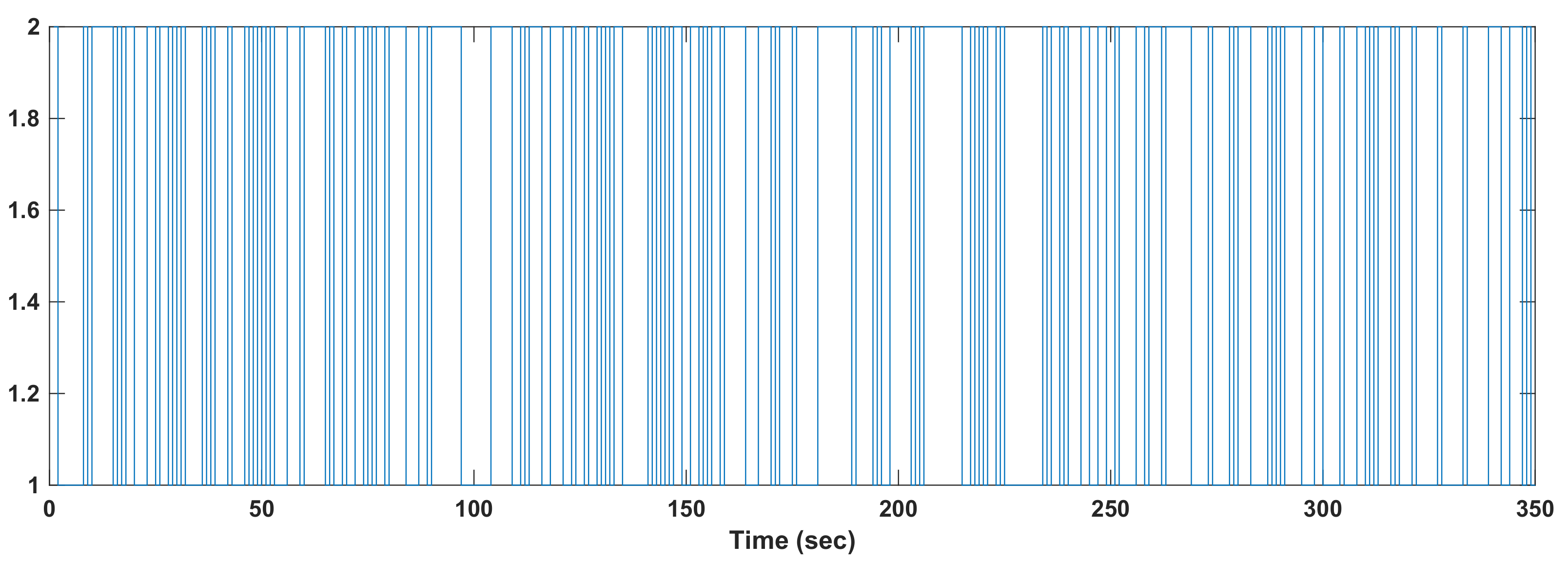
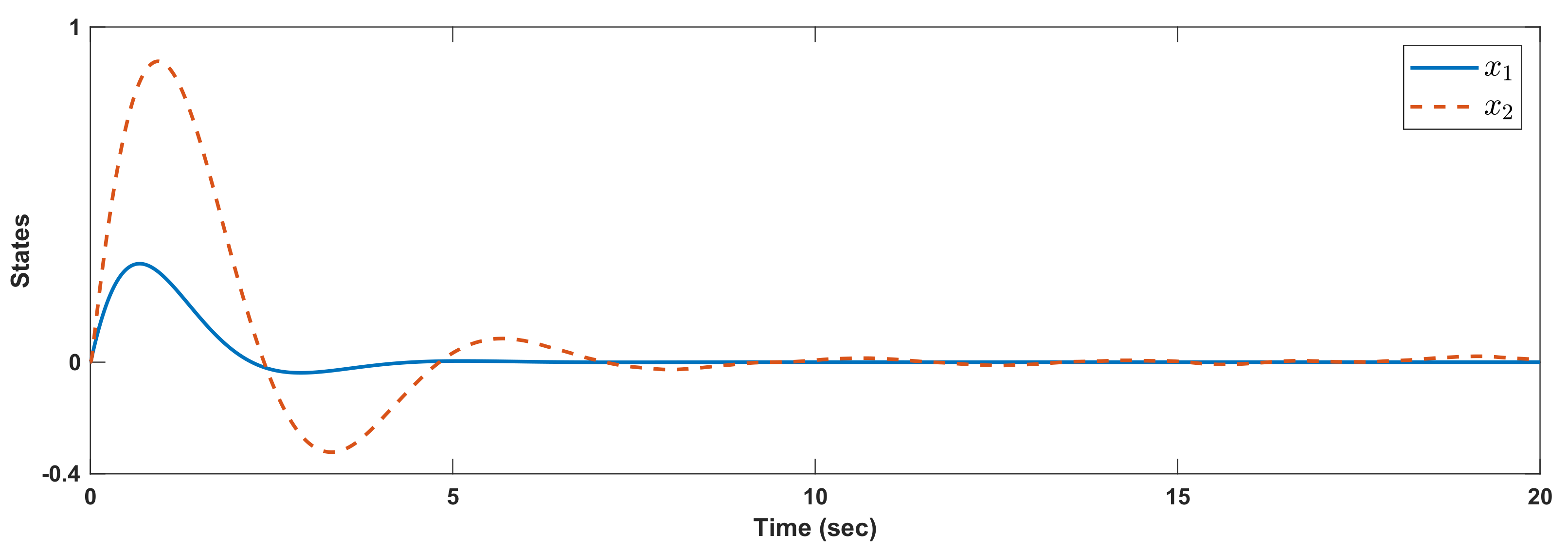
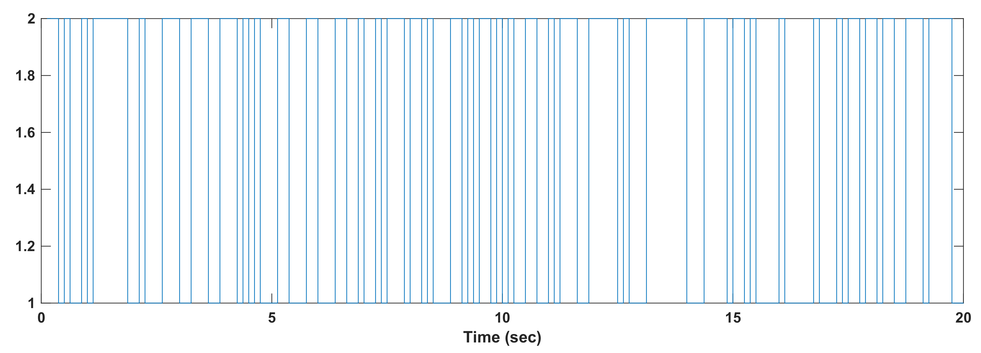
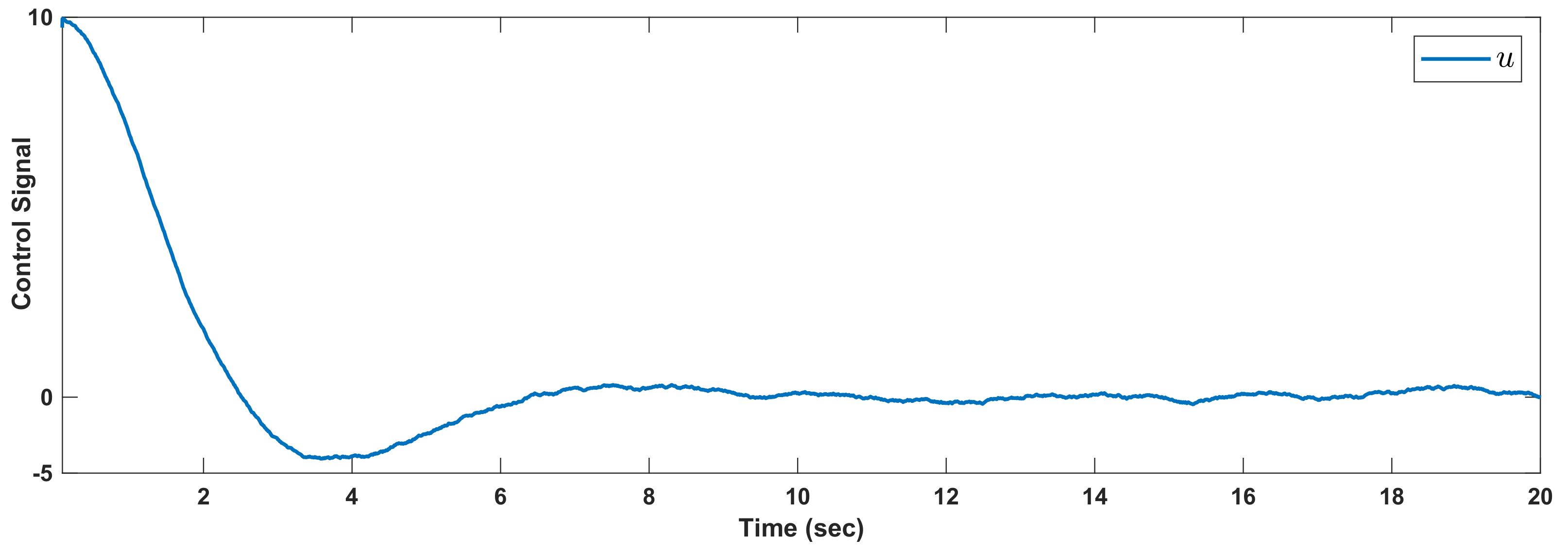
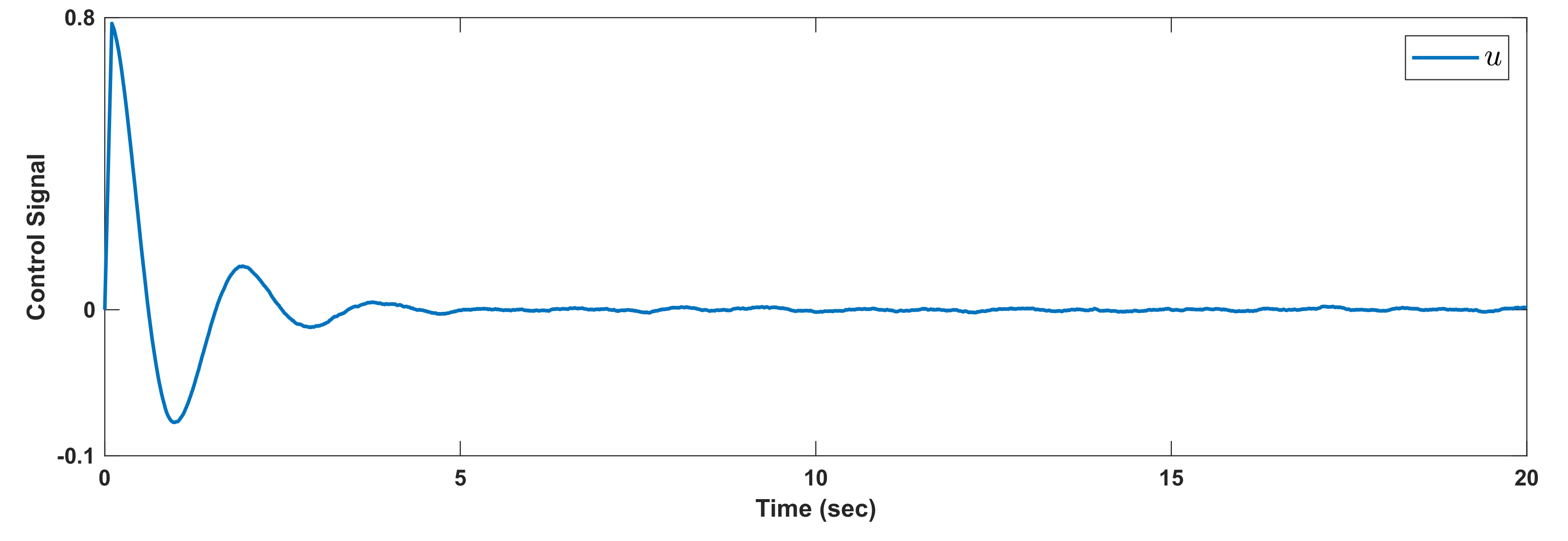
Designing $u\left(t\right)=K\left(r_t\right)\chi \left(t\right)$ and (1), one has

$$\begin{array}{c}\hfill \left\{\begin{array}{cc}\hfill & \dot{\chi }\left(t\right)=\left(\mathcal{A}\left(r_t\right)+\mathcal{B}\left(r_t\right)K\left(r_t\right)\right)\chi \left(t\right)+{\mathcal{A}}_d\left(r_t\right)\chi (t-\iota )\hfill \\ \hfill & \chi \left(t\right)=\mathsf{\Phi }\left(t\right)r\left(0\right)=r_{0}t\in [-\iota ,0].\hfill \end{array}\right.\end{array}$$

(33)

Additionally, in the LMI extracted in Theorem 2, due to open-loop stability analysis, we should only replace ${\mathcal{A}}_i$ with the ${\mathcal{A}}_i+{\mathcal{B}}_i{K}_i$ matrix. Thus, we will have:

$$\begin{array}{c}S\stackrel{\Delta }{=}\left[\begin{array}{cc}\left({\Theta }_i+{\overline{P}}_i\right)-{\mu }_{i}I& {\mu }_{i}I+F_i^T{\Psi }_i\\ & -{\mu }_{i}I\end{array}\right]<0i=1,2,\dots ,N\hfill \\ F_i=\left[\begin{array}{cccc}{\mathcal{A}}_i+{\mathcal{B}}_i{K}_i& {\mathcal{A}}_{di}& 0& -I\\ -I& -I& -I& 0\end{array}\right]\hfill \end{array}$$

(34)

On the other hand, in Theorems 2 and 3, it was said that ${\Psi }_i={\mu }_i{\Sigma }_i$, in which ${\Sigma }_i\in R^{2n\times 4n}$ is a matrix with an optional row rate, and the main structure of it will be chosen as below:

$${\Sigma }_i=\left[\begin{array}{cccc}{\Sigma }_{11i}& 0& 0& {\Sigma }_{14i}\\ {\Sigma }_{21i}& 0& 0& {\Sigma }_{24i}\end{array}\right].$$

(35)

In the following Theorem, the method of extracting interest of the state feedback controller due to nominal stability of the closed loop system is explained:

Theorem 4.

The system in relation (34) has the potential to change to random stability. If, for the given delay $\iota >0$, ${\Sigma }_{11i}$ and ${\Sigma }_{14i}$ matrices $M_{1i}$, $M_{2i}$, $N_i$, $P_i>0$, $Q>0$ and $Z>0$, and scalar ${\mu }_i>0$ exists in a way that the following LMIs can be established simultaneously:

$$\begin{array}{c}{\rm Y}\stackrel{\Delta }{=}\left[\begin{array}{cc}\left({\Theta }_i+{\overline{P}}_i\right)-{\mu }_{i}I& {\mu }_{i}I+{\mathsf{\Xi }}_i\\ & -{\mu }_{i}I\end{array}\right]<0i=1,2,\dots ,N\hfill \\ where:\hfill \\ {\mathsf{\Xi }}_i=\left[\begin{array}{cccc}{\mu }_i{\mathcal{A}}_i^T{\Sigma }_{11i}+N_i^T{B}_i^T{\Sigma }_{11i}+M_{1i}& 0& 0& {\mu }_i{\mathcal{A}}_i^T{\Sigma }_{14i}+N_i^T{B}_i^T{\Sigma }_{14i}+M_{2i}\\ {\mu }_i{\mathcal{A}}_{di}^T{\Sigma }_{11i}& 0& 0& {\mu }_i{\mathcal{A}}_{di}^T{\Sigma }_{14i}-M_{2i}\\ -M_{1i}& 0& 0& -M_{2i}\\ {\mu }_i{\Sigma }_{11i}& 0& 0& -{\mu }_i{\Sigma }_{14i}\end{array}\right]\hfill \end{array}$$

(36)

If the above LMI is affordable, controller $K_i$ is defined from the relation $K_i={\mu }_i^{-1}{N}_i$.

Proof. 

Where replacing ${\Sigma }_i$ is suggested from the relation in the $F_i^T{\Psi }_i$ matrix of LMI in relation (35), we will have ${\Psi }_i={\mu }_i{\Sigma }_i$ and

$$F_i^T{\Psi }_i=\left[\begin{array}{cccc}{\mu }_i{\mathcal{A}}_i^T{\Sigma }_{11i}+{\mu }_i{K}_i^T{B}_i^T{\Sigma }_{11i}+{\mu }_i{\Sigma }_{21i}& 0& 0& {\mu }_i{\mathcal{A}}_i^T{\Sigma }_{14i}+{\mu }_i{K}_i^T{B}_i^T{\Sigma }_{14i}+{\mu }_i{\Sigma }_{24i}\\ {\mu }_i{\mathcal{A}}_{di}^T{\Sigma }_{11i}& 0& 0& {\mu }_i{\mathcal{A}}_{di}^T{\Sigma }_{14i}-{\mu }_i{\Sigma }_{24i}\\ -{\mu }_i{\Sigma }_{21i}& 0& 0& -{\mu }_i{\Sigma }_{24i}\\ {\mu }_i{\Sigma }_{11i}& 0& 0& -{\mu }_i{\Sigma }_{14i}\end{array}\right].$$

(37)

Considering this point that choosing a ${\Sigma }_i$ matrix introduction is for the designer, ${\Sigma }_{11i}$ and ${\Sigma }_{14i}$ can be assumed as given (in other words, these two matrices are design parameters and their initialization data are defined by the designer). Additionally, ${\Sigma }_{21i}$ & ${\Sigma }_{24i}$ are undefined (these two matrices are free parameters). Now, applying the variables’ changes $N_i={\mu }_i{K}_i$, $M_{1i}={\mu }_i{\Sigma }_{21i}$, $M_{2i}={\mu }_i{\Sigma }_{24i}$, relation 31-3 will be a linear matrix according to parameters $N_i$, $M_{i1}$, $M_{i2}$, and ${\mu }_i$, which is in fact the defined ${\mathsf{\Xi }}_i$ in relation (37), and so the relation (37) is a type of LMI, and in the case of being affordable, the optimum values of anonymous parameters will be specified, and the interest of mode-dependent controllers will be defined from relation $K_i={\mu }_i^{-1}{N}_i$.

So far, we have managed to extract an optimal mode feedback controller to ensure closed loop stability for nominal systems mentioned in relation (34). In the next Theorem, the target is to generalize the obtained results for system equations in the presence of polytopic uncertainties. To gain this goal, assume ${\mathcal{A}}_i$, ${{\mathcal{A}}_d}_i$, ${\mathcal{B}}_i$ are undefined matrices but are related to the given ${\Lambda }_i$ multidimensional. In Theorem 3, we have proved that an open loop system in the presence of $\iota >0$ delay has random stability if ${\Psi }_i$, $P_i^{\left(r\right)}>0$, $Q^{\left(r\right)}>0$, $Z^{\left(r\right)}>0$ matrices exist for $i=1,2,\dots ,N$, in the way that the following LMIs are established simultaneously:

$$\begin{array}{c}S\stackrel{\Delta }{=}\left[\begin{array}{cc}\left({\Theta }_i^{\left(r\right)}+{\overline{P}}_i^{\left[{\pi }_{ir}\right]}\right)-{\mu }_i^{\left(r\right)}I& {\mu }_i^{\left(r\right)}I+F_{ir}^T{\Psi }_i\\ & -{\mu }_i^{\left(r\right)}I\end{array}\right]<0\hfill \\ i=1,2,\dots N,r=1,\dots ,{\nu }_i,\forall {\pi }_{ir}\in {\mathcal{I}}_{ir}\hfill \end{array}.$$

(38)

□

To stabilize the closed loop system, it is sufficient to replace ${\mathcal{A}}_{ir}+{\mathcal{B}}_{ir}{K}_i$ instead of ${\mathcal{A}}_{ir}$ in the $F_{ir}$ matrix, and the Theorem will be defined as below:

Theorem 5.

The system in relation (34) with a systemic matrix containing multidimensional uncertainty has randomly stable stability if, for $\iota >0$ delay ${\Sigma }_{11i}$, ${\Sigma }_{14i}$, the given $M_{1i}$, $N_i$, $P_i^{\left(r\right)}>0$, $Q^{\left(r\right)}>0$, $Z^{\left(r\right)}>0$, matrices and ${\mu }_i>0$ scalar for $i=1,2,\dots N$, $r=1,\dots ,{\nu }_i$ LMIs are established simultaneously:

$$\begin{array}{c}{\rm Y}\stackrel{\Delta }{=}\left[\begin{array}{cc}\left({\Theta }_i^{\left(r\right)}+{\overline{P}}_i^{\left[{\pi }_{ir}\right]}\right)-{\mu }_{i}I& {\mu }_{i}I+{\mathsf{\Xi }}_{ir}\\ & -{\mu }_{i}I\end{array}\right]<0\hfill \\ i=1,2,\dots ,N,r=1,\dots ,{\nu }_i,\forall {\pi }_{ir}\in {\mathcal{I}}_{ir}\hfill \\ where:\hfill \\ {\mathsf{\Xi }}_{ir}=\left[\begin{array}{cccc}{\mu }_i{\mathcal{A}}_{ir}^T{\Sigma }_{11i}+N_i^T{B}_{ir}^T{\Sigma }_{11i}+M_{1i}& 0& 0& {\mu }_i{\mathcal{A}}_{ir}^T{\Sigma }_{14i}+N_i^T{B}_{ir}^T{\Sigma }_{14i}+M_{2i}\\ {\mu }_i{\mathcal{A}}_{dir}^T{\Sigma }_{11i}& 0& 0& {\mu }_i{\mathcal{A}}_{dir}^T{\Sigma }_{14i}-M_{2i}\\ -M_{1i}& 0& 0& -M_{2i}\\ {\mu }_i{\Sigma }_{11i}& 0& 0& -{\mu }_i{\Sigma }_{14i}\end{array}\right]\hfill \\ {\Theta }_i^{\left(r\right)}=\left[\begin{array}{cccc}{Q}^{\left(r\right)}& 0& 0& P_i^{\left(r\right)}\\ & -Q^{\left(r\right)}& 0& 0\\ & *& -Z^{\left(r\right)}& 0\\ & *& *& {\iota }^2{Z}^{\left(r\right)}\end{array}\right]{\overline{P}}_i^{\left[{\pi }_{ir}\right]}=diag\left\{{\Pi }_i^T{\mathcal{P}}^{\left[{\pi }_{ir}\right]},0,0,0\right\}\hfill \end{array}.$$

(39)

If the above LMI is feasible, the $K_i$ controller is determined from the $K_i={\mu }_i^{-1}{N}_i$ relation.

Proof. 

The proof procedure is exactly the same as Theorem 3. We know that relation (37) LMIs in Theorem 4 that have been achieved for designing a randomized stabilizer controller closed loop system in the presence of delay are affine to the ${\mathsf{\Xi }}_{ir}$ matrix. Now, considering multidimensional uncertainty in systemic matrices and successive multiplication of relation (40) inequalities in ${\beta }_{jk}$ suitable scalars for their summation and repeating this method, this time-successive multiplication of the parties in ${\beta }_{ir}$ suitable scalars for $r=1,\dots ,{\nu }_i$ and their summation will have:

$$\begin{array}{c}\left[\begin{array}{cc}\left({\Theta }_i\left({\beta }_i\right)+{\overline{P}}_i^{\left[{\pi }_{ir}\right]}\left({\beta }_i\right)\right)-{\mu }_{i}I& {\mu }_{i}I+{\mathsf{\Xi }}_i\\ & -{\mu }_{i}I\end{array}\right]<0\hfill \\ \mathrm{where}:\hfill \\ {\mathcal{P}}^{\left[{\pi }_{ir}\right]}={\left[\begin{array}{ccccccc}{P}_1\left({\beta }_1\right)& \dots & P_{i-1}\left({\beta }_{i-1}\right)& P_i\left({\beta }_i\right)& P_{i+1}\left({\beta }_{i+1}\right)& \dots & P_N\left({\beta }_N\right)\end{array}\right]}^T\hfill \\ {\overline{P}}_i^{\left[{\pi }_{ir}\right]}\left({\beta }_i\right)=diag\left\{{\Pi }_i^T{\mathcal{P}}^{\left[{\pi }_{ir}\right]}\left({\beta }_i\right),0,0,0\right\}\hfill \end{array}.$$

(40)

In relation (40), it is seen that for any $({\mathcal{A}}_i,{\mathcal{A}}_{di},{\mathcal{B}}_i)\in {\Lambda }_i\mathrm{or}{\mathsf{\Xi }}_i\in {\Lambda }_i$ and $i=1,\dots N$ is confirmed in which a Lyapunov nominal matrix replaced with Lyapunov uncertainty matrices. Thus, in Theorem 5, we managed to achieve a sufficient condition with less conservation to relation (37) LMIs for designing a stable stabilizer controller due to ensuring randomized closed-loop stability under polytopic uncertainty in systemic matrices, and this section is thus also complete. □

7. Simulations

Example 1.

In this example, the stability of linear MJLS with nominal time delay is investigated.

In Theorem 2, we proved that system (1) is stable if, for delay $\iota >0$, there exists a full-rank matrix ${\Psi }_i$ and Laypunov matrices $P_i>0$, $Q>0$, $Z>0$ and scalar ${\mu }_i>0$ such that the LMI (23) is satisfied. A system with the following matrices is considered:

$$\begin{array}{c}{\mathrm{A}}_1=\left[\begin{array}{cc}-3.4888& 0.8057\\ -0.6451& -3.2684\end{array}\right]{\mathrm{A}}_2=\left[\begin{array}{cc}-2.4898& 0.2895\\ 1.3396& -0.0211\end{array}\right]\hfill \\ A_{d1}=\left[\begin{array}{cc}-0.862& -1.2919\\ -0.6841& -2.0729\end{array}\right]A_{d2}=\left[\begin{array}{cc}-2.8306& 0.4978\\ -0.8436& -1.0115\end{array}\right]\hfill \end{array}$$

(41)

where,

$$\Pi =\left[\begin{array}{cc}-6& 6\\ 8& -8\end{array}\right],\iota =0.756$$

(42)

For $\iota =0.756$, we obtain:

$$\begin{array}{c}P\left(1\right)=\left[\begin{array}{cc}0.1526& -0.0266\\ -0.0266& 0.0547\end{array}\right]P\left(2\right)=\left[\begin{array}{cc}0.1624& -0.0348\\ -0.0348& 0.0833\end{array}\right]\hfill \\ Z=\left[\begin{array}{cc}0.0213& 0.0158\\ 0.0158& 0.0118\end{array}\right]Q=\left[\begin{array}{cc}0.7928& -0.2758\\ -0.2758& 0.2050\end{array}\right]\hfill \\ \mu \left(1\right)=1.3635\mu \left(2\right)=1.0127\hfill \end{array}$$

(43)

For the initial condition ${\chi }_0={\left[\begin{array}{cc}1& 0.5\end{array}\right]}^T$, the results are shown in Figure 1. The Markovian changes are depicted in Figure 2.

It should be noted that, in comparison with the method of [37], the upper bound (UB) of the time delay is smaller than our method. In the LMI of [37], if $m=1$, the UB of the time delay is obtained as $\iota =0.377$. The other advantage of our method is that, in our LMIs, the systematic matrices are separated from Lyapunov matrices. Then, the conservatism of our approach in the presence of polytopic uncertainties is reduced.

Example 2.

In this example, the effectiveness of state feedback is evaluated. In Theorem (4), we proved that for delay $\iota >0$, asymptotic stability is ensured if $u\left(t\right)=K\left(r_t\right)\chi \left(t\right)$, and there exist $M_{1i}$, $M_{2i}$, $N_i$, $P_i>0$, $Q>0$, $Z>0$ and scalar ${\mu }_i>0$ such that LMIs (37) are satisfied. The system matrices are considered as:

$$\begin{array}{c}{\mathrm{A}}_1=\left[\begin{array}{cc}0.5& 0\\ 0& 0.75\end{array}\right]{\mathrm{A}}_{d1}=\left[\begin{array}{cc}-0.862& -1.2919\\ -0.6841& -2.0729\end{array}\right]B_1=\left[\begin{array}{c}0.5\\ 0.5\end{array}\right]\hfill \\ A_2=\left[\begin{array}{cc}0.5& 0\\ 0& 0.75\end{array}\right]A_{d2}=\left[\begin{array}{cc}-2.8306& 0.4978\\ -0.8436& -1.0115\end{array}\right]B_2=\left[\begin{array}{c}0.4\\ 0.8\end{array}\right]\hfill \end{array}$$

(44)

where,

$$\Pi =\left[\begin{array}{cc}-6& 6\\ 8& -8\end{array}\right]$$

(45)

For $\iota =0.1.05$, we obtain:

$$\begin{array}{c}P\left(1\right)=\left[\begin{array}{cc}0.1487& -0.1072\\ -0.1072& 0.1172\end{array}\right]P\left(2\right)=\left[\begin{array}{cc}0.1318& -0.0941\\ -0.0941& 0.1092\end{array}\right]\hfill \\ Z=\left[\begin{array}{cc}0.4497& -0.3714\\ -0.3714& 0.4921\end{array}\right]Q=\left[\begin{array}{cc}0.9511& -0.1457\\ -0.1457& 0.4721\end{array}\right]\hfill \\ \mu \left(1\right)=0.5875\mu \left(2\right)=0.6923\hfill \end{array}$$

(46)

$$\begin{array}{c}{\Sigma }_{11}\left(1\right)=\left[\begin{array}{cc}0.2509& -0.0973\\ -0.0973& 0.1138\end{array}\right]{\Sigma }_{14}\left(1\right)=\left[\begin{array}{cc}0.3811& -0.2439\\ -0.2439& 0.2264\end{array}\right]\hfill \\ {\Sigma }_{11}\left(2\right)=\left[\begin{array}{cc}0.3250& -0.1153\\ -0.1153& 0.1230\end{array}\right]{\Sigma }_{14}\left(2\right)=\left[\begin{array}{cc}0.2391& -0.1065\\ -0.1065& 0.1058\end{array}\right]\hfill \end{array}$$

(47)

By solving the LMIs, the feedback gains are obtained as:

$$\begin{array}{c}K\left(1\right)=\left[\begin{array}{cc}-0.5639& -1.0707\end{array}\right]\hfill \\ K\left(2\right)=\left[\begin{array}{cc}-0.8979& -4.3916\end{array}\right]\hfill \end{array}.$$

(48)

For the initial ${\chi }_0={\left[\begin{array}{cc}1& 0.5\end{array}\right]}^T$, the results are given in Figure 3. The Markovian changes are depicted in Figure 4. The control signal is given in Figure 5.

It should be noted that, in comparison with the method of [35], the UB of the time delay is smaller than our method. In the LMI of [35], the stability is proved for $\iota =0.47$, while in our suggested approach, we obtain $\iota =1.05$. We see that states are converged compared to the larger time delay.

Example 3.

In this example, the stability is investigated in the presence of ploytopic uncertainties. To consider ploytopic uncertainties, the system matrices are written as:

$${\Lambda }_i=\left\{\begin{array}{c}\left[\begin{array}{cc}{A}_i& \begin{array}{cc}{A}_{di}& B_i\end{array}\end{array}\right]|\left[\begin{array}{cc}{A}_i& \begin{array}{cc}{A}_{di}& B_i\end{array}\end{array}\right]=\hfill \\ \sum _{r=1}^{{\nu }_i}{\beta }_{ir}\left[\begin{array}{cc}{A}_{ir}& \begin{array}{cc}{A}_{dir}& B_{ir}\end{array}\end{array}\right];{\beta }_{ir}\ge 0,\sum _{r=1}^{{\nu }_i}{\beta }_{ir}=1\hfill \end{array}\right\}.$$

(49)

The matrices $A_{ir}$, $A_{dir}$ and $B_{ir}$ are known matrices. In Theorem 5, we proved that for delay $\iota >0$, the stability is ensured if there exist ${\Psi }_i$, $P_i^{\left(r\right)}>0$, $Q^{\left(r\right)}>0$, $Z^{\left(r\right)}>0$, ${\mu }_i^{\left(r\right)}>0$, such that the LMIs (40) are satisfied. For examination, the system matrices are considered as:

$$\begin{array}{c}{\mathrm{A}}_{11}=\left[\begin{array}{cc}-3.4888& 0.8057\\ -0.6451& -3.2684\end{array}\right]{\mathrm{A}}_{12}=\left[\begin{array}{cc}-3& 0.8057\\ -0.6& -2.7\end{array}\right]\hfill \\ {\mathrm{A}}_{21}=\left[\begin{array}{cc}-2.4898& 0.2895\\ 1.3396& -0.0211\end{array}\right]{\mathrm{A}}_{22}=\left[\begin{array}{cc}-2.4898& 0.2895\\ 1& 0\end{array}\right]\hfill \\ A_{d11}=\left[\begin{array}{cc}-0.862& -1.2919\\ -0.6841& -2.0729\end{array}\right]A_{d12}=\left[\begin{array}{cc}-0.7& -1\\ -0.5& -2.0729\end{array}\right]\hfill \\ A_{d21}=\left[\begin{array}{cc}-2.8306& 0.4978\\ -0.8436& -1.0115\end{array}\right]A_{d22}=\left[\begin{array}{cc}-2& 0.4978\\ -0.4& -1.0115\end{array}\right]\hfill \end{array}$$

(50)

where,

$$\Pi =\left[\begin{array}{cc}-6& 6\\ 8& -8\end{array}\right]$$

(51)

For time delay $\iota =0.62$, and initial condition ${\chi }_0={\left[\begin{array}{cc}1& 0.5\end{array}\right]}^T$, the results are given in Figure 6. The Markovian changes are depicted in Figure 7. The control signal is given in Figure 8. We see that ${\chi }_1$ and ${\chi }_2$ are converged compared to the time delay $\iota =0.62$ and polytopic uncertainties.

Example 4.

In this example, the feedback controller for MJLSs in the presence of polytopic uncertainties and time delay is evaluated. The details of stability are given in Theorem 5. The system matrices are considered as:

$$\begin{array}{c}{\mathrm{A}}_{11}=\left[\begin{array}{cc}-1.6& 0.8\\ -0.6& -1.5\end{array}\right]{\mathrm{A}}_{12}=\left[\begin{array}{cc}-1.4& 0.7\\ -0.6& -1.3\end{array}\right]\hfill \\ {\mathrm{A}}_{21}=\left[\begin{array}{cc}-1.4& 0.3\\ 1.3& 0\end{array}\right]{\mathrm{A}}_{22}=\left[\begin{array}{cc}-1.6& 0.3\\ 1.4& 0.1\end{array}\right]\hfill \\ A_{d11}=\left[\begin{array}{cc}-0.9& -1.3\\ -0.7& -2.1\end{array}\right]A_{d12}=\left[\begin{array}{cc}-1.1& -1.5\\ -0.8& -2.3\end{array}\right]\hfill \\ A_{d21}=\left[\begin{array}{cc}-2.3& 0.5\\ -0.8& -0.1\end{array}\right]A_{d22}=\left[\begin{array}{cc}-2.5& 0.6\\ -0.7& -0.2\end{array}\right]\hfill \\ B_{11}=\left[\begin{array}{c}1\\ 1\end{array}\right]B_{12}=\left[\begin{array}{c}1.1\\ 0.9\end{array}\right]\hfill \\ B_{21}=\left[\begin{array}{c}0\\ 1\end{array}\right]B_{22}=\left[\begin{array}{c}0.1\\ 0.9\end{array}\right]\hfill \end{array}$$

(52)

where,

$$\Pi =\left[\begin{array}{cc}-6& 6\\ 8& -8\end{array}\right]$$

(53)

For $\iota =0.74$, we obtain:

$$\begin{array}{c}{\Sigma }_{11}\left(1\right)=\left[\begin{array}{cc}0.3419& -0.0888\\ -0.0888& 0.2364\end{array}\right]{\Sigma }_{14}\left(1\right)=\left[\begin{array}{cc}0.2828& -0.0890\\ -0.0890& 0.1501\end{array}\right]\hfill \\ {\Sigma }_{11}\left(2\right)=\left[\begin{array}{cc}0.2061& -0.0016\\ -0.0016& 0.2652\end{array}\right]{\Sigma }_{14}\left(2\right)=\left[\begin{array}{cc}0.1428& -0.0092\\ -0.0092& 0.1830\end{array}\right]\hfill \end{array}$$

(54)

$$\begin{array}{c}K\left(1\right)=\left[\begin{array}{cc}-0.4358& -0.7116\end{array}\right]\hfill \\ K\left(2\right)=\left[\begin{array}{cc}-0.3768& -0.2166\end{array}\right]\hfill \end{array}$$

(55)

For initial condition ${\chi }_0={\left[\begin{array}{cc}1.4& 0.3\end{array}\right]}^T$, the results are given in Figure 9. The Markovian changes are depicted in Figure 10. The control signal is shown in Figure 11. We see that ${\chi }_1$ and ${\chi }_2$ are converged compared to time delay $\iota =0.74$ and polytopic uncertainties.

Remark 2.

The paper proposed a practical approach for MJSs, such that in addition to polytopic uncertainties, the effect of time delays was also considered. The conventional restrictions were made easier and the suggested controller can support more levels of time delays.

8. Conclusions

In this paper, the target was to analyze stochastic stability and design the stable stabilizer feedback controller for the delayed-MJLS systems in the presence of polytopic uncertainties. As it can be observed in the literature overview, systemic and polytopic matrices of the suggested Lyapunov-Krasovskii function exists in the extracted results of LMIs, and this causes more conservation for generalizing the polytopic uncertainty mode. For this target, in this paper, we managed to separate systemic matrices and Lyapunov matrices in the suggested Lyapunov-Krasovskii function to generalize the results of polytopic uncertainty with less conservation. The main results were divided into two main sections: stabilization analysis and feedback controller design for delayed MJSs. Four theorems were presented to give sufficient conditions to ensure stability in the presence of time delay and uncertainties. In simulation sections, four examples were presented to verify the obtained criteria. In the first example, the stability of a linear MJLS with nominal time delay was investigated. It is shown that the upper bound (UB) of time delay is bigger for our method in comparison with other conventional approaches. Additionally, in our LMIs, the systematic matrices were separated from Lyapunov matrices. Then, the conservatism of our approach in the presence of polytopic uncertainties was reduced. In the second example, the effectiveness of state feedback was evaluated. It was shown that the designed controller can support larger time delay. In the third example, the stability was investigated in the presence of polytopic uncertainties, and finally, in the last example, the feedback controller for MJLSs in the presence of polytopic uncertainties and time delay was evaluated. Simulation results show that the presented theorems are more effective, and in comparison with conventional methods, the stability was achieved in a higher upper bound of time delays. Additionally, it was shown that the conservative conditions became easier. For future studies, imperfections can be taken into consideration in switching with delay.

References

1. Rao, R.; Huang, J.; Yang, X. Global Stabilization of a Single-Species Ecosystem with Markovian Jumping under Neumann Boundary Value Via Laplacian Semigroup. Mathematics 2021, 9, 2446. [Google Scholar] [CrossRef]
2. Drăgan, V.; Ivanov, I.G.; Popa, I.L.; Bagdasar, O. Closed-Loop Nash Equilibrium in the Class of Piecewise Constant Strategies in a Linear State Feedback Form for Stochastic LQ Games. Mathematics 2021, 9, 2713. [Google Scholar] [CrossRef]
3. Liu, X.K.; Zhuang, J.J.; Li, Y. H Filtering for Markovian Jump Linear Systems with Uncertain Transition Probabilities. Int. J. Control Autom. Syst. 2021, 19, 2500–2510. [Google Scholar] [CrossRef]
4. Liu, X.; Teng, Y.; Yan, L. Finite-Time H Static Output Feedback Control for Itô Stochastic Markovian Jump Systems. Mathematics 2020, 8, 1709. [Google Scholar]
5. Wang, Y.; Pu, H.; Shi, P.; Ahn, C.K.; Luo, J. Sliding mode control for singularly perturbed Markov jump descriptor systems with nonlinear perturbation. Automatica 2021, 127, 109515. [Google Scholar] [CrossRef]
6. Krasovskii, N.; Lidskii, E. Analytical design of controllers in stochastic systems with velocity-limited controlling action. J. Appl. Math. Mech. 1961, 25, 627–643. [Google Scholar] [CrossRef]
7. Wonham, W.M. Random differential equations in control theory. Matematika 1973, 17, 129–167. [Google Scholar]
8. Blair, W., Jr.; Sworder, D. Feedback control of a class of linear discrete systems with jump parameters and quadratic cost criteria. Int. J. Control 1975, 21, 833–841. [Google Scholar] [CrossRef]
9. Rao, R.; Zhong, S. Input-to-state stability and no-inputs stabilization of delayed feedback chaotic financial system involved in open and closed economy. Discret. Contin. Dyn. Syst. S 2021, 14, 1375. [Google Scholar] [CrossRef] [Green Version]
10. Sworder, D.; Rogers, R. An LQ-solution to a control problem associated with a solar thermal central receiver. IEEE Trans. Autom. Control 1983, 28, 971–978. [Google Scholar] [CrossRef]
11. Dragan, V.; Ivanov, I.G. Sufficient conditions for Nash equilibrium point in the linear quadratic game for Markov jump positive systems. IET Control Theory Appl. 2017, 11, 2658–2667. [Google Scholar] [CrossRef]
12. Bucolo, M.; Buscarino, A.; Famoso, C.; Fortuna, L.; Frasca, M. Control of imperfect dynamical systems. Nonlinear Dyn. 2019, 98, 2989–2999. [Google Scholar] [CrossRef]
13. Loparo, K.; Abdel-Malek, F. A probabilistic approach to dynamic power system security. IEEE Trans. Circuits Syst. 1990, 37, 787–798. [Google Scholar] [CrossRef]
14. Dragan, V.; Aberkane, S. Robust stability of time-varying Markov jump linear systems with respect to a class of structured, stochastic, nonlinear parametric uncertainties. Axioms 2021, 10, 148. [Google Scholar] [CrossRef]
15. Cheng, P.; He, S.; Luan, X.; Liu, F. Finite-region asynchronous H control for 2D Markov jump systems. Automatica 2021, 129, 109590. [Google Scholar] [CrossRef]
16. Tian, Y.; Yan, H.; Zhang, H.; Cheng, J.; Shen, H. Asynchronous output feedback control of hidden semi-markov jump systems with random mode-dependent delays. IEEE Trans. Autom. Control in press. 2021. [CrossRef]
17. Xu, Y.; Wu, Z.G.; Sun, J. Security-Based Passivity Analysis of Markov Jump Systems via Asynchronous Triggering Control. IEEE Trans. Cybern. 2021, in press. [CrossRef]
18. Yao, X.; Zhang, L.; Zheng, W.X. Uncertain disturbance rejection and attenuation for semi-Markov jump systems with application to 2-degree-freedom robot arm. IEEE Trans. Circuits Syst. I Regul. Pap. 2021, 68, 3836–3845. [Google Scholar] [CrossRef]
19. Wang, Y.; Xia, J.; Shen, H.; Cao, J. HMM-based quantized dissipative control for 2-D Markov jump systems. Nonlinear Anal. Hybrid Syst. 2021, 40, 101018. [Google Scholar] [CrossRef]
20. Fang, H.; Zhu, G.; Stojanovic, V.; Nie, R.; He, S.; Luan, X.; Liu, F. Adaptive optimization algorithm for nonlinear Markov jump systems with partial unknown dynamics. Int. J. Robust Nonlinear Control 2021, 31, 2126–2140. [Google Scholar] [CrossRef]
21. Wan, H.; Karimi, H.R.; Luan, X.; Liu, F. Self-triggered finite-time H control for Markov jump systems with multiple frequency ranges performance. Inf. Sci. 2021, 581, 694–710. [Google Scholar] [CrossRef]
22. Wu, T.; Xiong, L.; Cao, J.; Park, J.H. Hidden Markov model-based asynchronous quantized sampled-data control for fuzzy nonlinear Markov jump systems. Fuzzy Sets Syst. 2021, in press. [CrossRef]
23. Hou, T.; Liu, Y.; Deng, F. Stability for discrete-time uncertain systems with infinite Markov jump and time delay. Sci. China Inf. Sci. 2021, 64, 1–11. [Google Scholar] [CrossRef]
24. Xie, W.; Nguang, S.K.; Zhu, H.; Zhang, Y.; Shi, K. A novel event-triggered asynchronous H control for TS fuzzy Markov jump systems under hidden Markov switching topologies. Fuzzy Sets Syst. 2021, in press. [CrossRef]
25. Lin, W.J.; Han, Q.L.; Zhang, X.M.; Yu, J. Reachable Set Synthesis of Markov Jump Systems with Time-Varying Delays and Mismatched Modes. IEEE Trans. Circuits Syst. II Express Briefs 2021, in press. [CrossRef]
26. Ma, C.; Fu, H.; Wu, W. Finite-time filtering of TS fuzzy semi-Markov jump systems with asynchronous mode-dependent delays. J. Frankl. Inst. 2021, in press.
27. Liu, L.J.; Zhang, X.; Zhao, X.; Yang, B. Stochastic finite-time stabilization for discrete-time positive Markov jump time delay systems. J. Frankl. Inst. 2021, in press. [CrossRef]
28. Liu, L.J.; Xu, N.; Zhao, X. Stability and L1-gain analysis of nonlinear positive Markov jump systems based on a switching transition probability. ISA Trans. 2021, in press. [CrossRef]
29. Liu, J.; Ran, G.; Huang, Y.; Han, C.; Yu, Y.; Sun, C. Adaptive Event-Triggered Finite-Time Dissipative Filtering for Interval Type-2 Fuzzy Markov Jump Systems With Asynchronous Modes. IEEE Trans. Cybern. 2021, in press. [CrossRef] [PubMed]
30. Ullah, S.; Khan, Q.; Mehmood, A.; Bhatti, A.I. Robust backstepping sliding mode control design for a class of underactuated electro–Mechanical nonlinear systems. J. Electr. Eng. Technol. 2020, 15, 1821–1828. [Google Scholar] [CrossRef]
31. Khan, Q. Integral backstepping based robust integral sliding mode control of underactuated nonlinear electromechanical systems. J. Control Eng. Appl. Inform. 2019, 21, 42–50. [Google Scholar]
32. Ullah, S.; Mehmood, A.; Ali, K.; Javaid, U.; Hafeez, G.; Ahmad, E. Dynamic Modeling and Stabilization of Surveillance Quadcopter in Space based on Integral Super Twisting Sliding Mode Control Strategy. In Proceedings of the 2021 International Conference on Artificial Intelligence (ICAI), IEEE, Islamabad, Pakistan, 5–7 April 2021; pp. 271–278. [Google Scholar]
33. Ullah, S.; Mehmood, A.; Khan, Q.; Rehman, S.; Iqbal, J. Robust integral sliding mode control design for stability enhancement of under-actuated quadcopter. Int. J. Control. Autom. Syst. 2020, 18, 1671–1678. [Google Scholar] [CrossRef]
34. Ullah, S.; Khan, Q.; Mehmood, A.; Kirmani, S.A.M.; Mechali, O. Neuro-adaptive fast integral terminal sliding mode control design with variable gain robust exact differentiator for under-actuated quadcopter UAV. ISA Trans. 2021, in press. [Google Scholar] [CrossRef] [PubMed]
35. Huang, H.; Feng, G.; Chen, X. Stability and stabilization of Markovian jump systems with time delay via new Lyapunov functionals. IEEE Trans. Circuits Syst. I Regul. Pap. 2012, 59, 2413–2421. [Google Scholar] [CrossRef]
36. Xia, Y.; Boukas, E.K.; Shi, P.; Zhang, J. Stability and stabilization of continuous-time singular hybrid systems. Automatica 2009, 45, 1504–1509. [Google Scholar] [CrossRef]
37. Gao, H.; Fei, Z.; Lam, J.; Du, B. Further results on exponential estimates of Markovian jump systems with mode-dependent time-varying delays. IEEE Trans. Autom. Control 2010, 56, 223–229. [Google Scholar] [CrossRef] [Green Version]
Figure 1. Example 1: Output trajectories.
Mathematics 10 00187 g001
Figure 2. Example 1: Markovian changes.
Mathematics 10 00187 g002
Figure 3. Example 2: Output trajectories.
Mathematics 10 00187 g003
Figure 4. Example 2: Markovian changes.
Mathematics 10 00187 g004
Figure 5. Example 2: Control signals.
Mathematics 10 00187 g005
Figure 6. Example 3: Output trajectories.
Mathematics 10 00187 g006
Figure 7. Example 3: Markovian changes.
Mathematics 10 00187 g007
Figure 8. Example 3: Control signals.
Mathematics 10 00187 g008
Figure 9. Example 4: Output trajectories.
Mathematics 10 00187 g009
Figure 10. Example 4: Markovian changes.
Mathematics 10 00187 g010
Figure 11. Example 4: Control signals.
Mathematics 10 00187 g011
Publisher’s Note: MDPI stays neutral with regard to jurisdictional claims in published maps and institutional affiliations.