Optimal Stabilization of Linear Stochastic System with Statistically Uncertain Piecewise Constant Drift

Abstract

The paper presents an optimal control problem for the partially observable stochastic differential system driven by an external Markov jump process. The available controlled observations are indirect and corrupted by some Wiener noise. The goal is to optimize a linear function of the state (output) given a general quadratic criterion. The separation principle, verified for the system at hand, allows examination of the control problem apart from the filter optimization. The solution to the latter problem is provided by the Wonham filter. The solution to the former control problem is obtained by formulating an equivalent control problem with a linear drift/nonlinear diffusion stochastic process and with complete information. This problem, in turn, is immediately solved by the application of the dynamic programming method. The applicability of the obtained theoretical results is illustrated by a numerical example, where an optimal amplification/stabilization problem is solved for an unstable externally controlled step-wise mechanical actuator.

1. Introduction

The linear quadratic Gaussian (LQG) control problem is one of the most productive results in the control theory. It represents the synthesis of a control law for a linear-Gaussian stochastic system state, which minimizes the expected value of a quadratic utility function [1]. The application area of the result is extremely broad: Aerospace applications were and still are important and include, for example, re-entry vehicle tracking and orbit determination [1]; other uses include navigation and guidance systems, radar tracking, and sonars, i.e., the same tasks that became the first applications for the Kalman filter [2]. Non-stationary technological objects management also became a significant source of applications. These industrial applications arise in paper and mineral processing industries, biochemistry and energy, and many other domains [3]. Industrial applications are often represented by very specific examples, for example, dry process rotary cement kiln, cement raw material mixing, and thickness control of a plastic film [4,5]. Of particular interest are the tasks connected with the mechanics of drives and manipulators, e.g., two-link manipulator stabilization [6] or output feedback stabilization for robot control [7]. In fact, these models do not have stochastic elements, but the applications served as a source of motivation for the present research.

One of the cornerstones of the contemporary LQG technique is the separation theorem, which is immanent to control problems with incomplete information [8,9]. This result justifies a transparent engineering approach, according to which the initial control problem splits into the unobservable state estimation stage and control synthesis based on the obtained state estimate. In the general nonlinear/non-Gaussian case, the separation procedure does not deliver an absolute optimum in the class of the admissible controls. Nevertheless, forcing the separation of the state estimation and control optimization allows synthesizing high-performance controls for various applied problems. This approach is called separation principle. Its applications are not only the aforementioned traditional tasks for applying Kalman filtering and LQG control. Recent applications cover rather modern areas, e.g., of telecommunications: In [10,11], LQG and Risk-Sensitive LQG controls are used in Denial-of-Service (DoS) attack conditions, and [12] uses similar models and tasks for control applications in lossy data networks. In [13], user activity measurements are used to manage computational resources of a data center or deep learning. In [14], the ideas of estimation and control separation are adapted for neural network training tasks. We can also note the development of the meaning of the term “separation”. In [15], for hybrid systems containing real-time control loops and logic-based decision makers, the control loops are separated. In [16], separation is interpreted in the sense that the output feedback controller is based on some separate properties related to state feedback on the one hand and output to state stability on the other hand.

Control problems with incomplete information, especially in stochastic settings, are usually of much higher relevance than those with complete information. The separation principle, being applied in a general control problem, provides a chance to use known theoretical results and corresponding numerical procedures developed for optimal stochastic control with complete information [17,18,19]. The separation principle implies the necessity to calculate a most precise state estimate given the available indirect noisy observations, which results in the optimal filtering problem. Its general solution, in turn, is characterized by either Kushner–Sratonovich [20,21] or Duncan–Mortensen–Zakai [22,23,24] equations, which describe posterior state distribution evolution in time. An approach developed in [25,26,27] results in easily calculated state estimates only in a limited number of special cases. Some examples can be found in [28] for a controlled Markov jump process (MJP).

For the quadratic criterion, the most general model where the separation theorem is valid was considered in [29,30,31]. The main goal of our research is to apply these results to a typical linear model of a mechanical actuator augmented by MJP to simulate changes in the actuator operating modes or external drift. The difference is that, in mentioned papers, there was no quadratic term involving the observed state; the criterion in [31] is more general but still does not include a term with an unobservable MJP. In this case, the obtained results provide an optimal control in the form of linear dependency on the observed state and the optimal estimate of the unobservable component. The latter is interpreted as an uncontrollable disturbance and is not included in the criterion. In the target application of our work, unobservable MJP represents the state of a controlled system. This state can be called an operating mode, and the purpose of control is to monitor this mode and to stabilize the system under the conditions determined by the mode switches. For the analysis of such a system, we do not need general models of the unobserved component as in [29,31] and the corresponding optimal filtering equations, which are difficult to implement in practice. For our purposes, an MJP model as in [30] and optimal Wonham filter [32] are sufficient. Thus, the main theoretical goal of our research is to develop the result of [30] for the case of a general quadratic criterion containing a term with unobservable MJP. The practical goal is to implement this statement in order to stabilize the mechanical actuator in conditions of changing operating modes.

The paper is organized as follows. Section 2 contains a thorough statement of an optimal control problem. The controlled observable output represents a solution to a linear stochastic differential system governed by some unobservable finite-state Markov jump process. The control appears on the right-hand side (RHS) as an additive term with some nonrandom matrix gain. The optimality criterion is a generalization of the traditional quadratic one. It allows investigating various optimal control problems (MJP state tracking in terms of integral performance index, control assistance in systems with noisy controls, damping of the statistically uncertain exogenous step-wise disturbances, etc.) using a unified approach.

On the one hand, a slight modification of the Wonham filter admits the calculation of the conditional expectation of an unobservable MJP state given output observations. On the other hand, the investigated dynamic system can be rewritten in form, which can be treated as a controlled system with complete information. In turn, the optimality criterion can be transformed to a form where the dependency on the unobserved MJP is only through its estimate. These manipulations, performed in Section 3 legitimize the usage of the separation principle in the investigated control problem (see Proposition 1).

Generally, in order to synthesize the optimal control, one has to solve the dynamic programming equation. However, the similarity of the considered control problem to the “classic” LQG case gives a hint for the form of the Bellman function. One can observe that it is a quadratic function of the controlled state. Hence, the problem is reduced to the characterization of corresponding coefficients. Section 4 and Section 5 contain their derivation.

Section 6 presents an illustrative example of the obtained theoretical results application. The object of the control is a mechanical actuator (e.g., the cart of a gantry crane). This actuator performs step-wise movements governed by an external unobservable controlling signal, which is an MJP corrupted by noise. The goal is the assistance of the actuator to carry out external commands more accurately. Section 7 contains concluding remarks.

2. Problem Statement

On the canonical probability space with filtration $\left(\mathsf{\Omega },\mathcal{F},\mathcal{P},{\mathcal{F}}_t\right)$, $t\in \left[0,T\right]$, we consider a partially observable stochastic dynamic system:

$$d{z}_t=a_t{y}_{t}dt+b_t{z}_{t}dt+c_t{u}_{t}dt+{\sigma }_{t}d{w}_t,z_0=Z,$$

(1)

$$d{y}_t={\mathsf{\Lambda }}_t^T{y}_{t}dt+d{\lambda }_t,y_0=Y,$$

(2)

where $z_t\in {\mathbb{R}}^{n_z}$ is an observable system state governed by a statistically uncertain (i.e., unobservable random) drift $y_t\in {\mathbb{R}}^{n_y}$. We suppose that $y_t$ is a finite-state Markov jump process (MJP) with values in the set $\{e_1,\dots ,e_{n_y}\}$ formed by unit coordinate vectors of the Euclidean space ${\mathbb{R}}^{n_y}$. The initial value Y has a known distribution ${\pi }_0$, ${\mathsf{\Lambda }}_t$ is a transition intensity matrix, and ${\lambda }_t$ is a ${\mathcal{F}}_t$-adapted martingale with quadratic characteristic [33].

$${〈\lambda ,\lambda 〉}_t={\int }_0^t\left(\mathrm{diag}\left\{{\mathsf{\Lambda }}_s^T{y}_s\right\}-{\mathsf{\Lambda }}_s^T\mathrm{diag}\left\{y_s\right\}-\mathrm{diag}\left\{y_s\right\}{\mathsf{\Lambda }}_s\right)ds.$$

We denote natural filtration generated by system state z as ${\mathcal{F}}_t^z$ and assume that ${\mathcal{F}}_t^z\subseteq {\mathcal{F}}_t\subseteq \mathcal{F}$. Furthermore, $w_t\in {\mathbb{R}}^{n_w}$ is a standard vector Wiener process. $Z\in {\mathbb{R}}^{n_z}$ is a random vector with a finite variance. Z, $\left\{y_t\right\}$, and $\left\{w_t\right\}$ are mutually independent; $u_t\in {\mathbb{R}}^{n_u}$ is an admissible control. We suppose that $u_t=u\left(t,z_t\right)$; thus, the admissible control is a feedback control: $u=u\left(t,z\right),$$z\in {\mathbb{R}}^{n_z}$ [19]. We also assume that state $z_t$ is uniformly non-degenerate, i.e., ${\sigma }_t{\sigma }_t^T⩾\kappa \mathbf{I}>0$, where $\kappa >0$ is some positive value, and $\mathbf{I}$ stands for a unit matrix of appropriate dimensionality.

The quality of the control law $U_0^T=\{u\left(t,z\right),0\le t\le T,z\in {\mathbb{R}}^{n_z}\}$ is defined by the following objective:

$$J\left(U_0^T\right)=\mathbb{E}\left\{{\int }_0^T{\left|P_t{y}_t+Q_t{z}_t+R_t{u}_t\right|}^{2}dt+{\left|P_T{y}_T+Q_T{z}_T\right|}^2\right\},$$

(3)

where $P_t\in {\mathbb{R}}^{n_J\times n_y}$, $Q_t\in {\mathbb{R}}^{n_J\times n_z}$, and $R_t\in {\mathbb{R}}^{n_J\times n_u}$ are known bounded matrix functions; ${\left|x\right|}^2=x^{T}x$ is the Euclidean norm of a vector x; and below we also use the Euclidean norm ${\left|x\right|}^2=\mathrm{tr}\left\{x^{T}x\right\}$ of a matrix x. In order to eliminate the possibility of zero penalties for individual components of the control vector $u_t$, which would make objective (3) physically incorrect, we assume that the common non-degeneracy assumption $R_t^T{R}_t⩾\kappa \mathbf{I}>0$ is valid.

Note that the stochastic system models (1) and (2) are the same as in [30] and are special cases of models in [29,31]. On the contrary, objective (3) includes additional terms. Namely, the objective from [29,30] is obtained at $P_t=0,Q_t=0$, and the one from [31] is obtained at $P_t=0$. This reflects the key terminological difference of the problem under consideration: We consider $y_t$ as an element of the observation system, external drift, and not as a complex measurement error. Thus, we represent objective (3), which may find its application in tracking the drift with state ${\left|y_t-z_t\right|}^2$ or tracking the drift with control ${\left|z_t-u_t\right|}^2$ problems, which take into account control ${\left|u_t\right|}^2$.

The matrix functions $a_t\in {\mathbb{R}}^{n_z\times n_y}$, $b_t\in {\mathbb{R}}^{n_z\times n_z}$, $c_t\in {\mathbb{R}}^{n_z\times n_u}$, and ${\sigma }_t\in {\mathbb{R}}^{n_z\times n_w}$ are bounded: $\left|a_t\right|+\left|b_t\right|+\left|c_t\right|+\left|{\sigma }_t\right|\le C$ for all $0\le t\le T$. Thus, the existence of a strong solution to (1) is guaranteed for any admissible control $u_t$. Moreover, we assume that all used time functions ${\mathsf{\Lambda }}_t$, $a_t$, $b_t$, $c_t$, ${\sigma }_t$, $P_t$, $Q_t$, $R_t$, and $S_t$ are piecewise continuous to ensure that the typical conditions for the existence of solutions to the ordinary differential equations (ODE) obtained below are satisfied.

Our goal is to find an admissible control ${\left(U^{*}\right)}_0^T=\{u^{*}\left(t,z\right),0\le t\le T,z\in {\mathbb{R}}^{n_z}\}$, which delivers the minimum to the quadratic criterion $J\left(U_0^T\right)$:

$${\left(U^{*}\right)}_0^T=arg\; minJ\left(U_0^T\right),$$

(4)

under the assumption of its existence.

3. Separation of Filtering and Control

In order to solve the problem formulated in Section 2, we need to transform it into a form that permits revealing two necessary properties. We note that for system (1) and (2) an optimal filtering problem solution is known: The expectation $\mathbb{E}\left\{y_t\right|{\mathcal{F}}_t^z\}$ is given by the Wonham filter [33]. First, for the separation, we need to find such a representation of this filter that shows that the quality of the optimal filter estimate does not depend on the chosen control law. The second goal is to decompose objective (3) into independent additive terms, which determine separately the quality of control and the quality of estimation.

To that end, we propose a change of variables in (1) to eliminate terms $b_t{z}_{t}dt$ and $c_t{u}_{t}dt$. Denote by $B_t\in {\mathbb{R}}^{n_z\times n_z}$ a solution to equation $d{B}_t=-B_t{b}_{t}dt$, which is the matrix exponential $B_t=exp\left\{-{\int }_0^t{b}_{s}ds\right\}$. Moreover, denote by $z_t^{\left(1\right)}\in {\mathbb{R}}^{n_z}$ the following linear output transform:

$$z_t^{\left(1\right)}=B_t{z}_t-{\int }_0^t{B}_s{c}_s{u}_{s}ds.$$

By differentiating, we obtain the following:

$$\begin{array}{cc}\hfill d{z}_t^{\left(1\right)}=& -B_t{b}_t{z}_{t}dt+B_{t}d{z}_t-B_t{c}_t{u}_{t}dt=\hfill \\ \hfill =& B_t\left(d{z}_t-b_t{z}_{t}dt-c_t{u}_{t}dt\right)=\hfill \\ \hfill =& B_t{a}_t{y}_{t}dt+B_t{\sigma }_{t}d{w}_t\hfill \end{array}$$

or

$$d{z}_t^{\left(1\right)}=a_t^{\left(1\right)}{y}_{t}dt+{\sigma }_t^{\left(1\right)}d{w}_t,z_0^{\left(1\right)}=Z,$$

(5)

with additional notation $a_t^{\left(1\right)}=B_t{a}_t$, ${\sigma }_t^{\left(1\right)}=B_t{\sigma }_t$.

Taking into account $B_t^{-1}=exp\left\{{\int }_0^t{b}_{s}ds\right\}$, for what follows, note the following:

$$B_t^{-1}d{z}_t^{\left(1\right)}=d{z}_t-b_t{z}_{t}dt-c_t{u}_{t}dt.$$

The transformations we made do not affect the filtering problem solution, i.e., $\mathbb{E}\left\{y_t|{\mathcal{F}}_t^z\right\}=\mathbb{E}\left\{y_t|{\mathcal{F}}_t^{z^{\left(1\right)}}\right\}$. That is because the change of variables used to obtain $z_t^{\left(1\right)}$ is a linear non-degenerate transformation of $z_t$. Hence, the optimal filtering estimate does not depend on $u_t$, and we can use $z_t^{\left(1\right)}$ as observations and obtain the same drift estimate no matter which admissible control law is chosen. Consequently, in place of the estimate problem given the control-dependent observations $z_t$, we pass to an equivalent problem of $y_t$ estimation given the transformed observations $z_t^{\left(1\right)}$, which are described by Equation (5) and do not depend on $u_t$.

Denoting the optimal estimate ${\widehat{y}}_t=\mathbb{E}\left\{y_t|{\mathcal{F}}_t^{z^{\left(1\right)}}\right\}$, we write the equation for it. The uniform non-degeneracy of ${\sigma }_t^{\left(1\right)}{\left({\sigma }_t^{\left(1\right)}\right)}^T$ along with the one of the matrix exponential $B_t$ [34] legitimizes the use of the Wonham filter [33]:

$$\begin{array}{ccc}\hfill d{\widehat{y}}_t=& {\mathsf{\Lambda }}_t^T{\widehat{y}}_{t}dt+\left(\mathrm{diag}\left\{{\widehat{y}}_t\right\}-{\widehat{y}}_t{\widehat{y}}_t^T\right){\left(a_t^{\left(1\right)}\right)}^T{\left({\sigma }_t^{\left(1\right)}{\left({\sigma }_t^{\left(1\right)}\right)}^T\right)}^{-1}\times \hfill & \\ \hfill & \times \left(d{z}_t^{\left(1\right)}-a_t^{\left(1\right)}{\widehat{y}}_{t}dt\right),{\widehat{y}}_0=\mathbb{E}\left\{Y\right\}.\hfill \end{array}$$

Replacing variables $a_t^{\left(1\right)}$, ${\sigma }_t^{\left(1\right)}$, and $z_t^{\left(1\right)}$, we obtain the following:

$$\begin{array}{ccc}\hfill d{\widehat{y}}_t=& {\mathsf{\Lambda }}_t^T{\widehat{y}}_{t}dt+\left(\mathrm{diag}\left\{{\widehat{y}}_t\right\}-{\widehat{y}}_t{\widehat{y}}_t^T\right)a_t^T{B}_t^T{\left(B_t{\sigma }_t{\sigma }_t^T{B}_t^T\right)}^{-1/2}\times \hfill & \\ \hfill & \times {\left(B_t{\sigma }_t{\sigma }_t^T{B}_t^T\right)}^{-1/2}{B}_t\left(B_t^{-1}d{z}_t^{\left(1\right)}-a_t{\widehat{y}}_{t}dt\right)=\hfill \\ \hfill =& {\mathsf{\Lambda }}_t^T{\widehat{y}}_{t}dt+\left(\mathrm{diag}\left\{{\widehat{y}}_t\right\}-{\widehat{y}}_t{\widehat{y}}_t^T\right)a_t^T{B}_t^T{\left(B_t{\sigma }_t{\sigma }_t^T{B}_t^T\right)}^{-1}{B}_t\times \hfill & \\ \hfill & \times \left(d{z}_t-b_t{z}_{t}dt-c_t{u}_{t}dt-a_t{\widehat{y}}_{t}dt\right).\hfill \end{array}$$

Taking into account $B_t^T{\left(B_t{\sigma }_t{\sigma }_t^T{B}_t^T\right)}^{-1}{B}_t={\left({\sigma }_t{\sigma }_t^T\right)}^{-1}$, we have the final representation for the Wohnam filter as follows:

$$\begin{array}{ccc}\hfill d{\widehat{y}}_t=& {\mathsf{\Lambda }}_t^T{\widehat{y}}_{t}dt+\left(\mathrm{diag}\left\{{\widehat{y}}_t\right\}-{\widehat{y}}_t{\widehat{y}}_t^T\right)a_t^T{\left({\sigma }_t{\sigma }_t^T\right)}^{-1/2}\times \hfill & \\ \hfill & \times {\left({\sigma }_t{\sigma }_t^T\right)}^{-1/2}\left(d{z}_t-b_t{z}_{t}dt-c_t{u}_{t}dt-a_t{\widehat{y}}_{t}dt\right),{\widehat{y}}_0=\mathbb{E}\left\{Y\right\},\hfill \end{array}$$

(6)

where

$$d{W}_t={\left({\sigma }_t{\sigma }_t^T\right)}^{-1/2}\left(d{z}_t-b_t{z}_{t}dt-c_t{u}_{t}dt-a_t{\widehat{y}}_{t}dt\right)$$

is a differential of the ${\mathcal{F}}_t^z$-adapted standard vector Wiener process. This provides us the final observation equation:

$$d{z}_t=a_t{\widehat{y}}_{t}dt+b_t{z}_{t}dt+c_t{u}_{t}dt+{\widehat{\sigma }}_{t}d{W}_t,$$

(7)

where ${\widehat{\sigma }}_t={\left({\sigma }_t{\sigma }_t^T\right)}^{1/2},$ and the final new state equation is as follows:

$$d{\widehat{y}}_t={\mathsf{\Lambda }}_t^T{\widehat{y}}_{t}dt+\left(\mathrm{diag}\left\{{\widehat{y}}_t\right\}-{\widehat{y}}_t{\widehat{y}}_t^T\right)a_t^T{\left({\sigma }_t{\sigma }_t^T\right)}^{-1/2}d{W}_t.$$

(8)

Furthermore, by denoting the following:

$${\mathsf{\Sigma }}_t={\mathsf{\Sigma }}_t\left(y\right)=\left(\mathrm{diag}\left\{y\right\}-y{y}^T\right)a_t^T{\left({\sigma }_t{\sigma }_t^T\right)}^{-1/2},y\in {\mathbb{R}}^{n_y},$$

we obtain a control system with complete information:

$$\begin{array}{cc}d{z}_t=a_t{\widehat{y}}_{t}dt+b_t{z}_{t}dt+c_t{u}_{t}dt+\widehat{{\sigma }_t}d{W}_t,\hfill & z_0=Z,\hfill \\ d{\widehat{y}}_t={\mathsf{\Lambda }}_t^T{\widehat{y}}_{t}dt+{\mathsf{\Sigma }}_t\left({\widehat{y}}_t\right)d{W}_t,\hfill & {\widehat{y}}_0=\mathbb{E}\left\{Y\right\},\hfill \end{array}$$

(9)

where both variables ${\widehat{y}}_t$ and $z_t$ are observable.

For final formulation of the equivalent control problem, one needs to perform the change of variables in objective (3). This can be conducted by using the law of total expectation [35] as follows:

$$J\left(U_0^T\right)=\mathbb{E}\left\{\begin{array}{c}{\int }_0^T{\left|P_t\left(y_t-{\widehat{y}}_t+{\widehat{y}}_t\right)+Q_t{z}_t+R_t{u}_t\right|}^{2}dt+\\ +{\left|P_T\left(y_T-{\widehat{y}}_T+{\widehat{y}}_T\right)+Q_T{z}_T\right|}^2\end{array}\right\}$$

$$=\mathbb{E}\left\{\begin{array}{c}{\int }_0^T{\left|P_t{\widehat{y}}_t+Q_t{z}_t{+R}_t{u}_t\right|}^{2}dt+{\left|P_T{\widehat{y}}_T+Q_T{z}_T\right|}^2+\\ +{\int }_0^T{\left|P_t\left(y_t-{\widehat{y}}_t\right)\right|}^{2}dt+{\left|P_T\left(y_T-{\widehat{y}}_T\right)\right|}^2\end{array}\right\}.$$

Since the last additive term in the expression for $J\left(U_0^T\right)$ does not depend on $U_0^T$ but merely characterises the quality of the optimal filter estimate ${\widehat{y}}_t$, it can be excluded from the criterion. Hence, the new objective takes the following form:

$$J\left(U_0^T\right)=\mathbb{E}\left\{{\int }_0^T{\left|P_t{\widehat{y}}_t+Q_t{z}_t{+R}_t{u}_t\right|}^{2}dt+{\left|P_T{\widehat{y}}_T+Q_T{z}_T\right|}^2\right\}.$$

(10)

The final statement is formulated as follows.

Proposition 1

(Separation theorem). The optimal (${\mathcal{F}}_t^{\widehat{y},z}$-adapted) feedback control for the system with complete information (9) and objective (10) is at the same time an optimal (${\mathcal{F}}_t^z$-adapted) solution for the optimal control problem in the original system (1) and (2) with objective (3).

Note that control ${\left(U^{*}\right)}_0^T$ minimizes both functionals (10) and (3), and the difference

$${\int }_0^T{\left|P_t\left(y_t-{\widehat{y}}_t\right)\right|}^{2}dt+{\left|P_T\left(y_T-{\widehat{y}}_T\right)\right|}^2$$

between $J\left(U_0^T\right)$ from (10) and $J\left(U_0^T\right)$ from (3) does not depend on $U_0^T$; thus, there is no need for another notation for the objective.

4. Solution to Control Problem

In order to find the control for the system (9), which is optimal with respect to the criterion (3), we use the classical dynamic programming method [18,19].

Denote the following Bellman function:

$$V_t=V_t\left(y,z\right)=\underset{U_t^T}{inf}\mathbb{E}\left\{{\int }_t^T{\left|P_s{\widehat{y}}_s+Q_s{z}_s{+R}_s{u}_s\right|}^{2}ds+{\left|P_T{\widehat{y}}_T+Q_T{z}_T\right|}^2\right\},$$

where $U_t^T=\{u\left(s,y,z\right),t\le s\le T,y\in {\mathbb{R}}^{n_y},z\in {\mathbb{R}}^{n_z}\}$. Then, with ${\mathsf{\Sigma }}_t={\mathsf{\Sigma }}_t\left(y\right)$ the dynamic programming equation is as follows:

$$\begin{array}{c}{\displaystyle \frac{\partial V_t}{\partial t}+\frac{1}{2}\mathrm{tr}\left\{{\mathsf{\Sigma }}_t^T\frac{{\partial }^2{V}_t}{\partial y^2}{\mathsf{\Sigma }}_t+{\widehat{\sigma }}_t^T\frac{{\partial }^2{V}_t}{\partial z^2}{\widehat{\sigma }}_t+2{\mathsf{\Sigma }}_t^T\frac{{\partial }^2{V}_t}{\partial y\partial z}{\widehat{\sigma }}_t\right\}}\hfill \\ {\displaystyle +\underset{u}{min}\left\{y^T{\mathsf{\Lambda }}_t\frac{\partial V_t}{\partial y}+{\left(a_{t}y+b_{t}z+c_{t}u\right)}^T\frac{\partial V_t}{\partial z}+{\left|P_{t}y+Q_{t}z{+R}_{t}u\right|}^2\right\}=0,}\hfill \\ {\displaystyle V_T={\left|P_{T}y+Q_{T}z\right|}^2,}\hfill \end{array}$$

(11)

where admissible feedback control $u=u\left(t,y,z\right)$ corresponds to system (9) designations; thus, $u_t=u\left(t,{\widehat{y}}_t,z_t\right)$. Note that this is the same control that appeared in the original statement, since ${\widehat{y}}_t={\widehat{y}}_t\left(z_t\right)$.

The existence of a solution to (11) is a sufficient optimality condition. Moreover, the optimal control is the one that minimizes to the corresponding additive term. Hence, under condition $R_t^T{R}_t⩾\alpha I>0$ and under the assumption of (11) solution existence, this minimum is delivered by the following control:

$$u^{*}=u^{*}(t,y,z)=-\frac{1}{2}{\left(R_t^T{R}_t\right)}^{-1}\left(c_t^T\frac{\partial V_t}{\partial z}+2R_t^T\left(P_{t}y+Q_{t}z\right)\right).$$

(12)

By substituting $u_t^{*}$ in (11) and regrouping the additive terms, we obtain the following:

$$\begin{array}{c}{\displaystyle \frac{\partial V_t}{\partial t}+\frac{1}{2}\mathrm{tr}\left\{{\mathsf{\Sigma }}_t^T\frac{{\partial }^2{V}_t}{\partial y^2}{\mathsf{\Sigma }}_t+{\widehat{\sigma }}_t^T\frac{{\partial }^2{V}_t}{\partial z^2}{\widehat{\sigma }}_t+2{\mathsf{\Sigma }}_t^T\frac{{\partial }^2{V}_t}{\partial y\partial z}{\widehat{\sigma }}_t\right\}+y^T{\mathsf{\Lambda }}_t\frac{\partial V_t}{\partial y}}\hfill \\ {\displaystyle +\left(y^T{a}_t^T+z^T{b}_t^T-{\left(R_t^T\left(P_{t}y+Q_{t}z\right)\right)}^T{\left(R_t^T{R}_t\right)}^{-1}{c}_t^T\right)\frac{\partial V_t}{\partial z}}\hfill \\ {\displaystyle +{\left(P_{t}y+Q_{t}z\right)}^T\left(\mathbf{I}-R_t{\left(R_t^T{R}_t\right)}^{-1}{R}_t^T\right)\left(P_{t}y+Q_{t}z\right)}\hfill \\ {\displaystyle -\frac{1}{4}{\left(\frac{\partial V_t}{\partial z}\right)}^T{c}_t{\left(R_t^T{R}_t\right)}^{-1}{c}_t^T\frac{\partial V_t}{\partial z}=0.}\hfill \end{array}$$

(13)

The linear observations (9) and quadratic objective (10) suggest that a solution of the dynamic programming Equation (13) might be presented as follows:

$$V_t=V_t\left(y,z\right)=z^T{\alpha }_{t}z+z^T{\beta }_t\left(y\right)+{\gamma }_t\left(y\right),$$

(14)

which reduces the optimal solution search to a problem of finding a symmetric matrix function ${\alpha }_t$, vector function ${\beta }_t\left(y\right)$, and a scalar ${\gamma }_t\left(y\right)$. Moreover, the explicit representation for ${\gamma }_t\left(y\right)$ is not necessary for optimal control. One only needs a derivative $\frac{\partial V_t}{\partial z}=2{\alpha }_{t}z+{\beta }_t\left(y\right)$; nevertheless, ${\gamma }_t\left(y\right)$ will be useful in determining the quality of control.

The Bellman function representation (14) can be simplified further by using the fact that the term with derivative $\frac{\partial V_t}{\partial y}$ in (13) contains only the multiplier $y_t{\mathsf{\Lambda }}_t^T$. This suggests that ${\beta }_t\left(y\right)$ is an affine transform of y:

$${\beta }_t\left(y\right)={\mathcal{B}}_{t}y,$$

(15)

where matrix ${\mathcal{B}}_t\in {\mathbb{R}}^{n_z\times n_y}$. The boundary condition at the same time takes the following form:

$$V_T={\left|P_{T}y+Q_{T}z\right|}^2=z^T{Q}_T^T{Q}_{T}z+2z^T{Q}_T^T{P}_{T}y+y^T{P}_T^T{P}_{T}y,$$

In other words, we have the following:

$${\alpha }_T=Q_T^T{Q}_T,{\mathcal{B}}_T=2Q_T^T{P}_T,{\gamma }_T\left(y\right)=y^T{P}_T^T{P}_{T}y,$$

(16)

and the optimal control (12) can finally be represented as

$$u^{*}=u^{*}(t,y,z)=-\frac{1}{2}{\left(R_t^T{R}_t\right)}^{-1}\left(c_t^T\left(2{\alpha }_{t}z+{\mathcal{B}}_{t}y\right)+2R_t^T\left(P_{t}y+Q_{t}z\right)\right).$$

(17)

Thus, $u_t^{*}$ contains two terms: The first term is linear in observations (output variable) z; the second one is linear in state (state estimate given by Wonham filter) y. In order to justify the assumptions made, it is necessary to derive ${\alpha }_t$, ${\mathcal{B}}_t$, and ${\gamma }_t\left(y\right)$ such that under assumptions (14) and (15) made about the Bellman function $V_t$ and the affinity of ${\beta }_t\left(y\right)$, $V_t$ from (14) would in fact be a solution of (13). To that end, we substitute (14) into Equation (13) and take into account that the derivatives of ${\beta }_t\left(y\right)$ according to (15) are equal to $\frac{{\partial }^2{\beta }_t\left(y\right)}{\partial y^2}=0,$ $\frac{\partial {\beta }_t\left(y\right)}{\partial y}={\mathcal{B}}_t^T,$ and also that the following is the case:

$$y^T{\mathsf{\Lambda }}_t\frac{\partial V_t}{\partial y}={\left(\frac{\partial V_t}{\partial y}\right)}^T{\mathsf{\Lambda }}_t^{T}y=z^T{\mathcal{B}}_t{\mathsf{\Lambda }}_t^{T}y+y^T{\mathsf{\Lambda }}_t\frac{\partial {\gamma }_t\left(y\right)}{\partial y},\frac{{\partial }^2{V}_t}{\partial y\partial z}={\mathcal{B}}_t^T.$$

After this substitution and minor transformations, grouping the terms at $z^T$ and z, at $z^T$ and at $z^0$, we obtain equations for ${\alpha }_t$, ${\beta }_t\left(y\right)={\mathcal{B}}_{t}y$ and ${\gamma }_t={\gamma }_t\left(y\right)$, respectively:

$$\frac{d{\alpha }_t}{dt}+M_t^{\alpha }{\alpha }_t+{\alpha }_t{\left(M_t^{\alpha }\right)}^T+N_t^{\alpha }-{\alpha }_t{c}_t{\left(R_t^T{R}_t\right)}^{-1}{c}_t^T{\alpha }_t=0,$$

(18)

$$\frac{d{\mathcal{B}}_t}{dt}y+{\mathcal{B}}_t{\mathsf{\Lambda }}_t^{T}y+M_t^{\beta }y+N_t^{\beta }{\mathcal{B}}_{t}y=0,$$

(19)

$$\frac{\partial {\gamma }_t}{\partial t}+\frac{1}{2}\mathrm{tr}\left\{{\mathsf{\Sigma }}_t^T\frac{{\partial }^2{\gamma }_t}{\partial y^2}{\mathsf{\Sigma }}_t\right\}+\mathrm{tr}\left\{{\widehat{\sigma }}_t^T{\alpha }_t{\widehat{\sigma }}_t+{\mathsf{\Sigma }}_t^T{\mathcal{B}}_t^T{\widehat{\sigma }}_t\right\}+y^T{\mathsf{\Lambda }}_t\frac{\partial {\gamma }_t}{\partial y}+M_t^{\gamma }\left(y\right)=0,$$

(20)

where the following is the case:

$$\begin{array}{ccc}\hfill {\displaystyle M_t^{\alpha }}& =& b_t^T-{Q_t^T{R}_t\left(R_t^T{R}_t\right)}^{-1}{c}_t^T,\hfill \\ \hfill {\displaystyle N_t^{\alpha }}& =& Q_t^T\left(\mathbf{I}-R_t{\left(R_t^T{R}_t\right)}^{-1}{R}_t^T\right)Q_t,\hfill \\ \hfill {\displaystyle M_t^{\beta }}& =& 2\left({\alpha }_t\left(a_t-{c_t\left(R_t^T{R}_t\right)}^{-1}{R}_t^T{P}_t\right)+Q_t^T\left(\mathbf{I}-R_t{\left(R_t^T{R}_t\right)}^{-1}{R}_t^T\right)P_t\right),\hfill \\ \hfill {\displaystyle N_t^{\beta }}& =& b_t^T-Q_t^T{R}_t{\left(R_t^T{R}_t\right)}^{-1}{c}_t^T-{\alpha }_t{c}_t{\left(R_t^T{R}_t\right)}^{-1}{c}_t^T,\hfill \\ \hfill {\displaystyle M_t^{\gamma }\left(y\right)}& =& y^T{\mathcal{B}}_t^T\left(a_t-c_t{\left(R_t^T{R}_t\right)}^{-1}{R}_t^T{P}_t\right)y+y^T{P}_t^T\left(\mathbf{I}-R_t{\left(R_t^T{R}_t\right)}^{-1}{R}_t^T\right)P_{t}y\hfill \\ \hfill {\displaystyle }& & -\frac{1}{4}{y}^T{\mathcal{B}}_t^T{c}_t{\left(R_t^T{R}_t\right)}^{-1}{c}_t^T{\mathcal{B}}_{t}y.\hfill \end{array}$$

Finally, from (19), we obtain the equation for ${\mathcal{B}}_t$:

$$\frac{d{\mathcal{B}}_t}{dt}+{\mathcal{B}}_t{\mathsf{\Lambda }}_t^T+M_t^{\beta }+N_t^{\beta }{\mathcal{B}}_t=0.$$

(21)

The obtained equations are solved with boundary conditions (16). In this case, Equation (18) is a matrix Riccati equation for a square symmetric matrix ${\alpha }_t$. The above assumptions regarding the piecewise continuity of the coefficients of this equation and condition $R_t^T{R}_t>0$ are sufficient for the existence and uniqueness of a positive semidefinite solution for every $0\le t\le T$. Indeed, such an equation occurs in the classical linear-quadratic problem, which admits a unique optimal feedback control—linear with respect to the output $Z_t$—and with a gain described by this Riccati equation [36].

Equation (21) is a system of linear ODEs with respect to variable $B_t$ with piecewise continuous coefficients; hence, the existence and uniqueness of a solution is ensured by the usual theorem for linear differential equations [37].

Equation (20) for ${\gamma }_t\left(y\right)$ is a linear partial differential equation of parabolic type, but unlike the equation for ${\beta }_t\left(y\right)$, it can not be simplified. We will assume that this equation has a solution, and we interpret this assumption as a sufficient condition the same as the above dynamic programming Equation (11).

The following statement summarizes the reasoning in the section.

Proposition 2

(Output control under complete information). If the dynamic programming Equation (11) solution exists, then this solution admits representation (14), (15) with coefficients ${\alpha }_t$, ${\mathcal{B}}_t$, and ${\gamma }_t\left(y\right)$ given by (18), (21), and (20), respectively, and the optimal control $u^{*}$ is given by (17).

5. Stochastic Representation of Gamma Functional

In order to implement control (12), one needs functions ${\alpha }_t$ and ${\mathcal{B}}_t$. These can be calculated by means of any effective numerical method of ODE solution; hence, the practical solution of Equations (18) and (21) presents no difficulties. At the same time, the quality of optimal control is given by a solution of the dynamic programming equation:

$$J\left({\left(U^{*}\right)}_0^T\right)=V_0\left(Y,Z\right)=\mathbb{E}\left\{Z^T{\alpha }_{0}Z+Z^T{\mathcal{B}}_{0}Y+{\gamma }_0\left(Y\right)\right\},$$

Therefore, functional ${\gamma }_t\left(y\right)$ is also required. An approximate solution to (20) can be also obtained numerically by traditional grid methods, especially since these methods are well studied for equations of parabolic type. Nevertheless, growth of the dimensionality of Y may cause certain difficulties. However, the main thing is that, for Equation (20), there is only an initial condition ${\gamma }_T\left(y\right)$ defined by (16), more precisely, a terminal condition, and there is no boundary condition such as ${\gamma }_t\left(y_{max}\right)$, which is necessary for numerical treatments.

That is why, in our opinion, an alternative approach based on the known relation between solutions of partial differential equations of parabolic type and stochastic equations is more promising. An example of such relation is the Kolmogorov equation [38], which determines the connection between the solution of the Cauchy problem with the terminal condition for the parabolic equation, on the one hand, and the solution of the related stochastic equation, on the other hand. Moreover, here, we need a simpler integral representation of the solution of a parabolic equation, known as the Feynman–Kac formula [39]. The application of such tools for the numerical solution of parabolic equations has been well studied in a more general setting than we need [40].

For differential Equation (20), the Feynman–Kac formula has the following form:

$${\gamma }_t\left(y\right)=\mathbb{E}\left\{{\widehat{y}}_T^T{P}_T^T{P}_T{\widehat{y}}_T+{\int }_t^T{M}_{\tau }^{\gamma }\left({\widehat{y}}_{\tau }\right)d\tau |{\mathcal{F}}_t^y\right\}.$$

(22)

Here, we deliberately use the same notation for two different random processes:

• Random process, which generates a terminal condition under the mathematical expectation and passes through point $\left(t,y\right):{\widehat{y}}_t=y$;
• The Wonham filter estimate, which substitutes the state in observation Equation (9).

This emphasizes the fact that both these processes are described by the same equation and have the same probabilistic characteristics.

For practical applications of (22), we rewrite this relation by adding an auxiliary variable ${\widehat{y}}_t^{\gamma }$ in a differential form:

$$\begin{array}{c}{\displaystyle d{\widehat{y}}_{\tau }={\mathsf{\Lambda }}_{\tau }^T{\widehat{y}}_{\tau }d\tau +{\mathsf{\Sigma }}_{\tau }\left({\widehat{y}}_{\tau }\right)d{W}_{\tau },{\widehat{y}}_t=y,t\le \tau \le T,}\\ {\displaystyle \frac{d{\widehat{y}}_{\tau }^{\gamma }}{d\tau }=M_{\tau }^{\gamma }\left({\widehat{y}}_{\tau }\right)d\tau ,{\widehat{y}}_t^{\gamma }=0,}\\ {\displaystyle {\gamma }_t\left(y\right)=\mathbb{E}\left\{{\widehat{y}}_T^T{P}_T^T{P}_T{\widehat{y}}_T+{\widehat{y}}_T^{\gamma }\right\}.}\end{array}$$

(23)

First, (23) is a stochastic representation of ${\gamma }_t\left(y\right)$, which explains the meaning of this coefficient. Secondly, (23) provides a basis for an approximate calculation of this coefficient. To be more precise, the proposed method of the numerical calculation of coefficient ${\gamma }_t\left(y\right)$ consists in applying the Monte Carlo method to system (23). To be more specific, one needs a series of sample solutions of this system for different initial conditions $\left(t,y\right)$ in order to obtain an approximate value of ${\gamma }_t\left(y\right)$ as a statistical estimate of the terminal condition in (23).

6. Assistance of Mechanical Actuator Control

We investigate a controllable mechanical actuator designed for step-wise movement. Its model is described by the following dynamic system:

$$\begin{array}{c}d\left(\begin{array}{c}{x}_t\\ v_t\end{array}\right)=\left(\begin{array}{cc}0& 1\\ a& b\end{array}\right)\left(\begin{array}{c}{x}_t\\ v_t\end{array}\right)dt-\hfill \\ \hfill -\left(\begin{array}{ccc}0& 0& 0\\ c_1& c_2& c_3\end{array}\right)y_{t}dt+\left(\begin{array}{c}0\\ h\end{array}\right)u_{t}dt+\left(\begin{array}{c}0\\ \sqrt{g}\end{array}\right)d{w}_t,t\in (0,T],\end{array}$$

(24)

$$\left(\begin{array}{c}{x}_0\\ v_0\end{array}\right)\sim \mathcal{N}\left(\left(\begin{array}{c}0\\ 0\end{array}\right),\left(\begin{array}{cc}{\sigma }_x^2& 0\\ 0& {\sigma }_v^2\end{array}\right)\right).$$

Here, we have the following:

• $x_t\in {\mathbb{R}}^1$ is an observable actuator position;
• $v_t\in {\mathbb{R}}^1$ is an observable actuator velocity;
• $y_t\in \left\{e_1,e_2,e_3\right\}$ is an unobservable external control action, supposed to be an MJP with known transition intensity matrix $\mathsf{\Lambda }$ and initial distribution vector ${\pi }_0$;
• $w_t\in {\mathbb{R}}^1$ is an external control noise supposed to be a standard Wiener process;
• $u_t\in {\mathbb{R}}^1$ is an admissible assisting control.

Thus, in the original notation, we have three-dimensional external unobservable control $y_t$ corrupted by the one-dimensional Wiener noise $w_t$, two-dimensional observable state vector $z_t=\mathrm{col}(x_t,v_t)$, and one-dimensional control $u_t$. The other notations are as follows:

$$a_t=-\left(\begin{array}{ccc}0& 0& 0\\ c_1& c_2& c_3\end{array}\right),b_t=\left(\begin{array}{cc}0& 1\\ a& b\end{array}\right),c_t=\left(\begin{array}{c}0\\ h\end{array}\right),{\sigma }_t=\left(\begin{array}{c}0\\ \sqrt{g}\end{array}\right).$$

It is easy to verify that in the case of noiseless (i.e., $g=0$) external constant control action $y_t\equiv e_j$, the actuator coordinate $x_t$ tends to its steady-state value $C_j=\frac{c_j}{a}$ as $t\to \infty$. Without loss of generality, we suppose that all components of vector $\mathbf{C}=\mathrm{row}(\frac{c_1}{a},\frac{c_2}{a},\frac{c_3}{a})$ are different.

In the case of piecewise constant control action $y_t$ and constant $g>0$, the mechanical actuator cannot implement the expected “ideal” step-wise trajectory $\mathbf{C}{y}_t$ due to the inertia and noise accompanying the external control. Thus, the aim of the assisting control $u_t$ is to improve actuator performance, and the corresponding criterion has the following form:

$$J\left(U_0^T\right)=\mathbb{E}\left\{{\int }_0^T\left({(\mathbf{C}{y}_t-x_t)}^2+R{u}_t^2\right)dt+\frac{1}{T}{(\mathbf{C}{y}_T-x_T)}^2\right\}\to \underset{U_0^T}{min},$$

(25)

where $R>0$ is a dimensionless unit cost of the assisting control.

We perform the calculations for the following parameter values:

$$\mathsf{\Lambda }=\left(\begin{array}{ccc}-0.5& 0.5& 0\\ 0.5& -1& 0.5\\ 0& 0.5& -0.5\end{array}\right);{\pi }_0=\left(\begin{array}{c}1\\ 0\\ 0\end{array}\right),$$

$$a=-1,b=-0.5,T=10,h=10,g=0.01,{\sigma }_x=1,{\sigma }_v=1,R=0.01,$$

$$\left(\begin{array}{ccc}{c}_1& c_2& c_3\end{array}\right)=\left(\begin{array}{ccc}1& 0& -1\end{array}\right),\mathbf{C}=\left(\begin{array}{ccc}{C}_1& C_2& C_3\end{array}\right)=\left(\begin{array}{ccc}-1& 0& 1\end{array}\right).$$

Stochastic system (24) is solved by the Euler–Maruyama numerical scheme with step $0.01$; meanwhile, Equations (18) and (21) are solved using the implicit Euler’s scheme with the same step.

Note, that the violation of condition ${\sigma }_t{\sigma }_t^T>0$ in (24) does not prevent the use of the obtained result, since coordinate $x_t$ in the state $z_t$ is a simple integral of the velocity $v_t$; thus, in the filtering problem, one can use only observation $v_t$.

It is easy to verify that the actuator is stable if $b<0$ and $b^2+4a<0$. In the example, we investigate only the stable case.

Figure 1, Figure 2 and Figure 3 present assisting control coefficients.

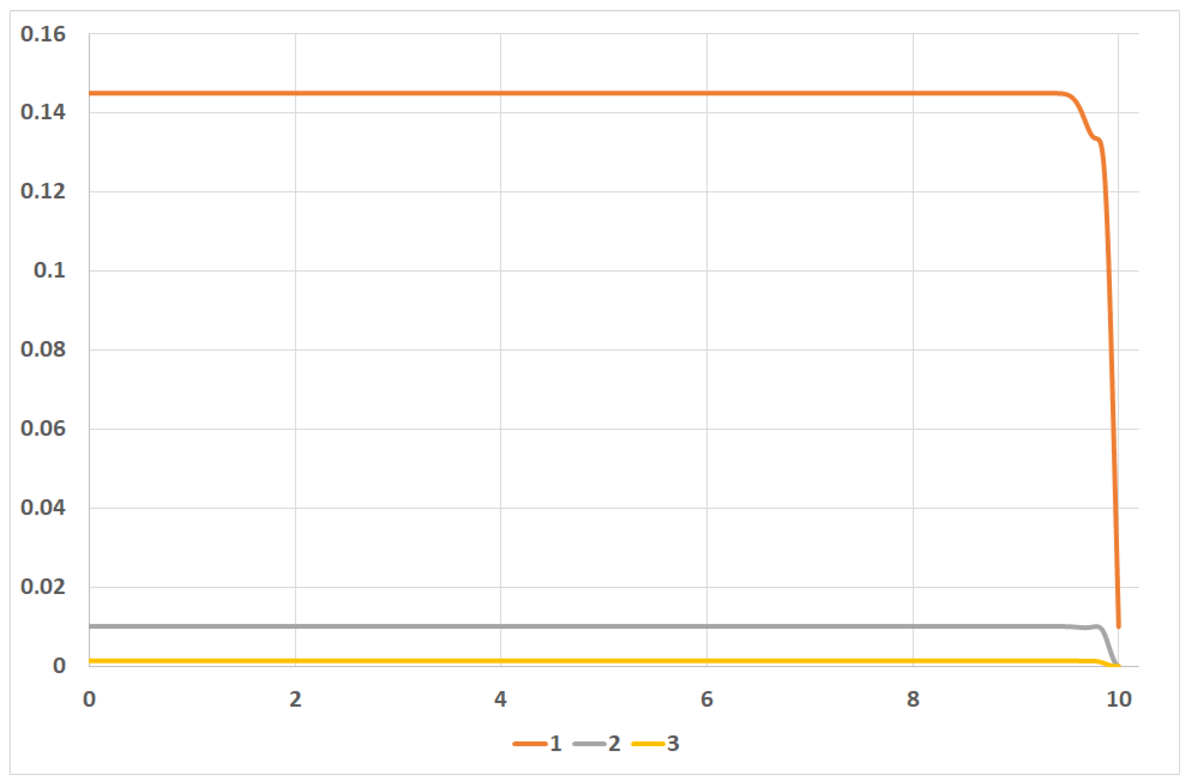
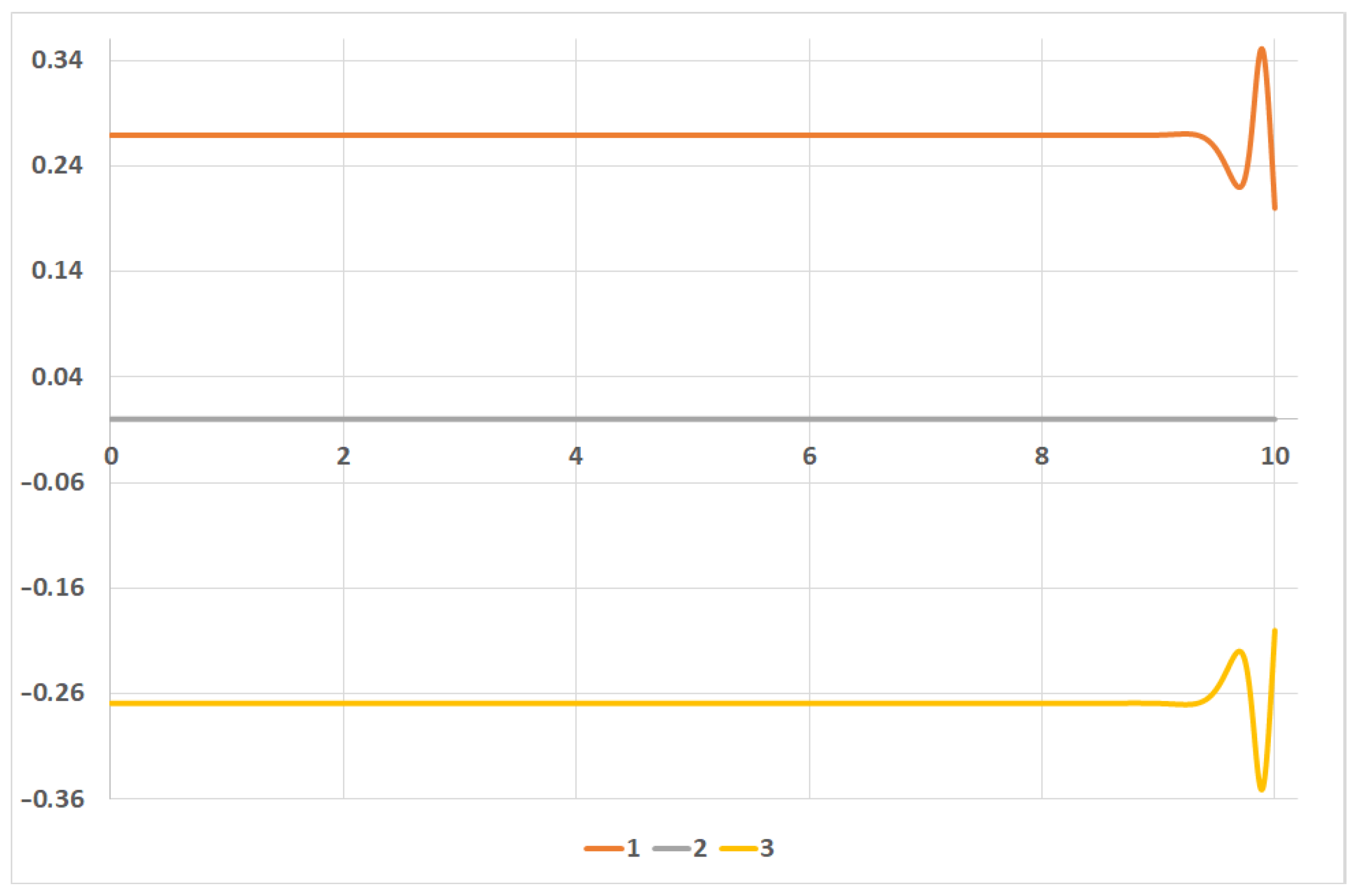
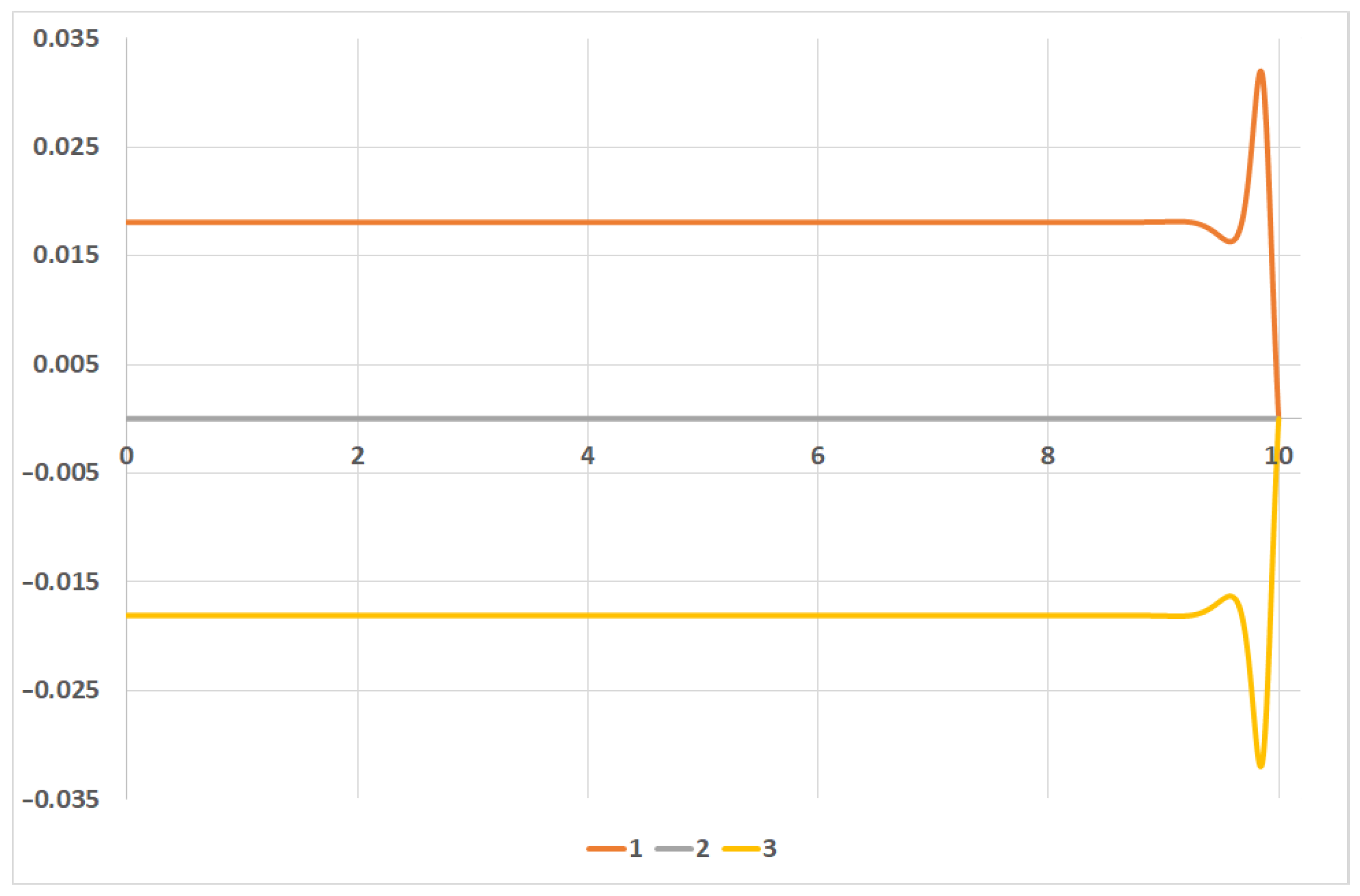
Figure 1 contains plots of the evolution in time for coefficients ${\alpha }_t^{\left(11\right)}$, ${\alpha }_t^{\left(12\right)}$, and ${\alpha }_t^{\left(22\right)}$; Figure 2 stands for coefficients ${\mathcal{B}}_t^{\left(11\right)}$, ${\mathcal{B}}_t^{\left(12\right)}$ and ${\mathcal{B}}_t^{\left(13\right)}$; Figure 3 stands for coefficients ${\mathcal{B}}_t^{\left(21\right)}$, ${\mathcal{B}}_t^{\left(22\right)}$ and ${\mathcal{B}}_t^{\left(23\right)}$. Here, we denote by $x^{\left(ij\right)}$ the element of matrix x with indexes $i,j$.

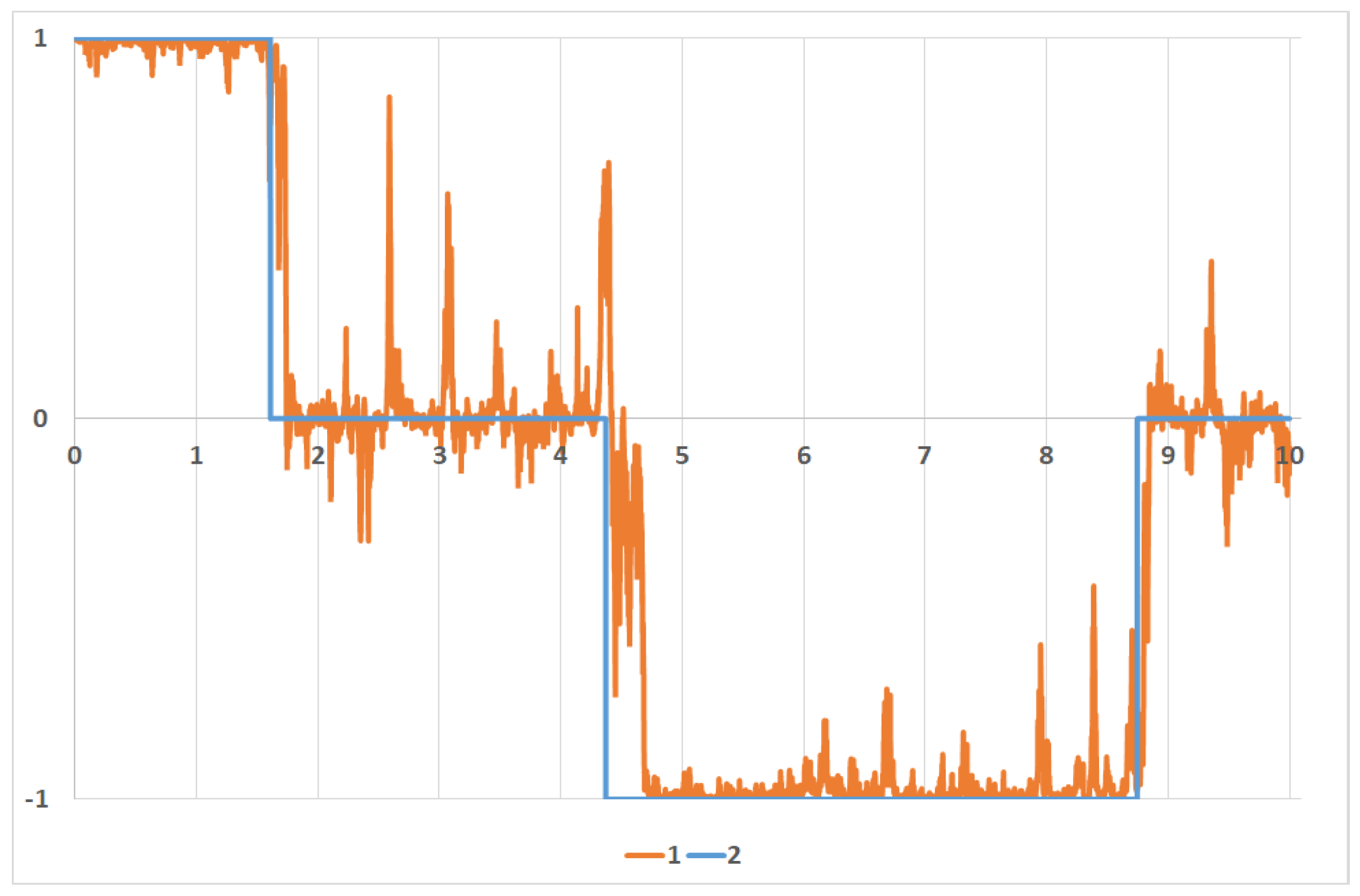
Figure 4 presents the comparison of the unobserved external control term $c{y}_t$ and its estimate $c{\widehat{y}}_t$ calculated by the Wonham filter.

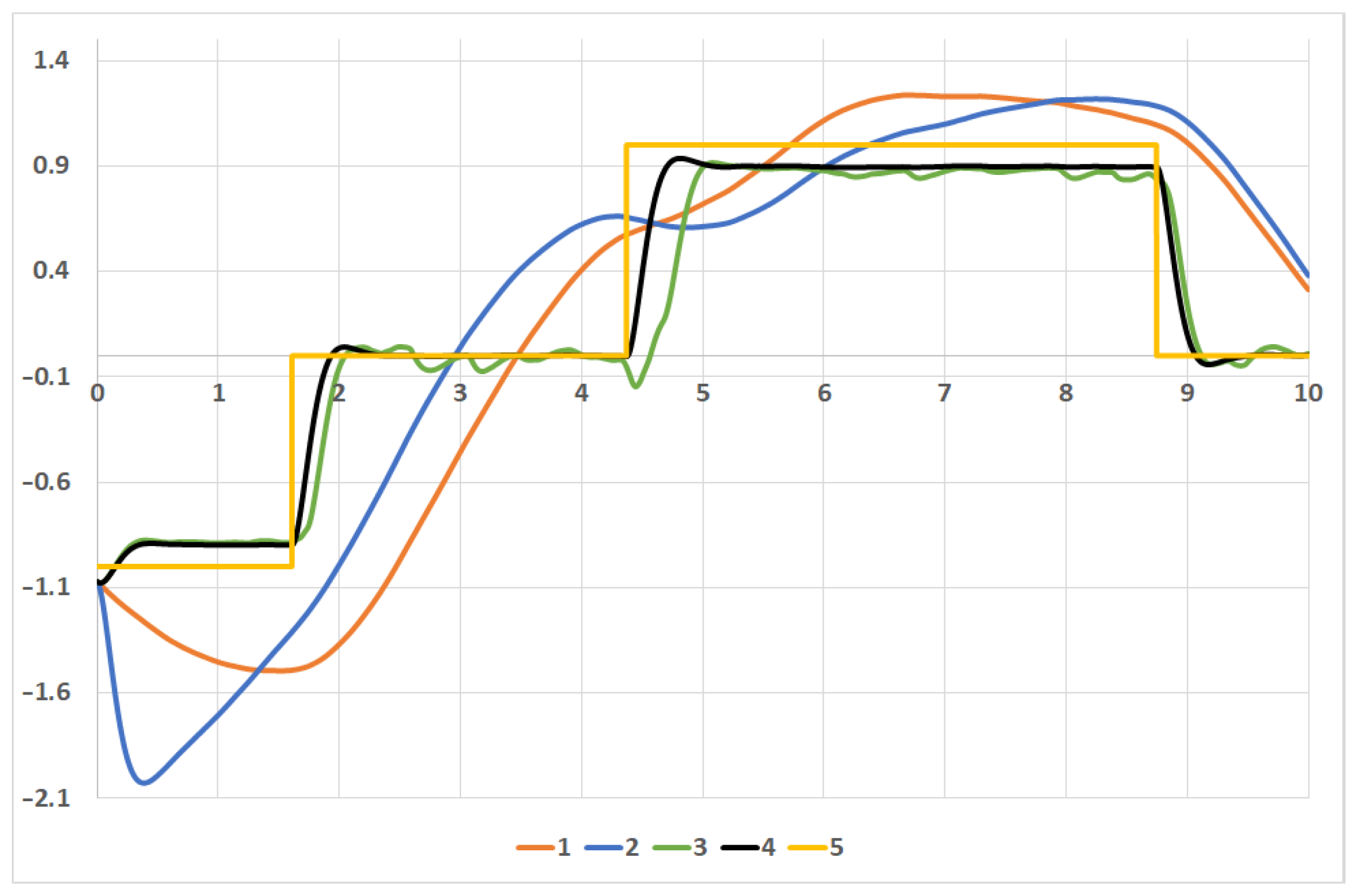
Figure 5 contains plots of the actuator coordinate governed by various types of assisting control:

• $x_t^{\left(0\right)}$ obtained without assisting control, i.e., for $u_t=u_t^{\left(0\right)}\equiv 0$;
• $x_t^{me}$ obtained under the trivial assisting control, i.e., for $u_t=u_t^{me}\equiv u^{*}(t,y_t^{me},z_t^{me}),$ where control law $u^{*}(t,y,z)$ is defined in (17), $y_t^{me}=\mathbb{E}\left\{y_t\right\}$, $z_t^{me}=\mathbb{E}\left\{z_t\right\}$;
• the optimal trajectory $x_t^{*}$ calculated for the optimal control $u_t=u_t^{*}$;
• the ”ideal” trajectory $x_t^{**}$ calculated for control $u_t=u_t^{**}\equiv u^{*}(t,y_t,z_t^{**}),$ i.e., optimal control law $u^{*}$ defined in (17) with full information $y=y_t$, $z=z_t^{**}$.

A comparison with the step-wise “target” trajectory $\mathbf{C}{y}_t$ is conducted.

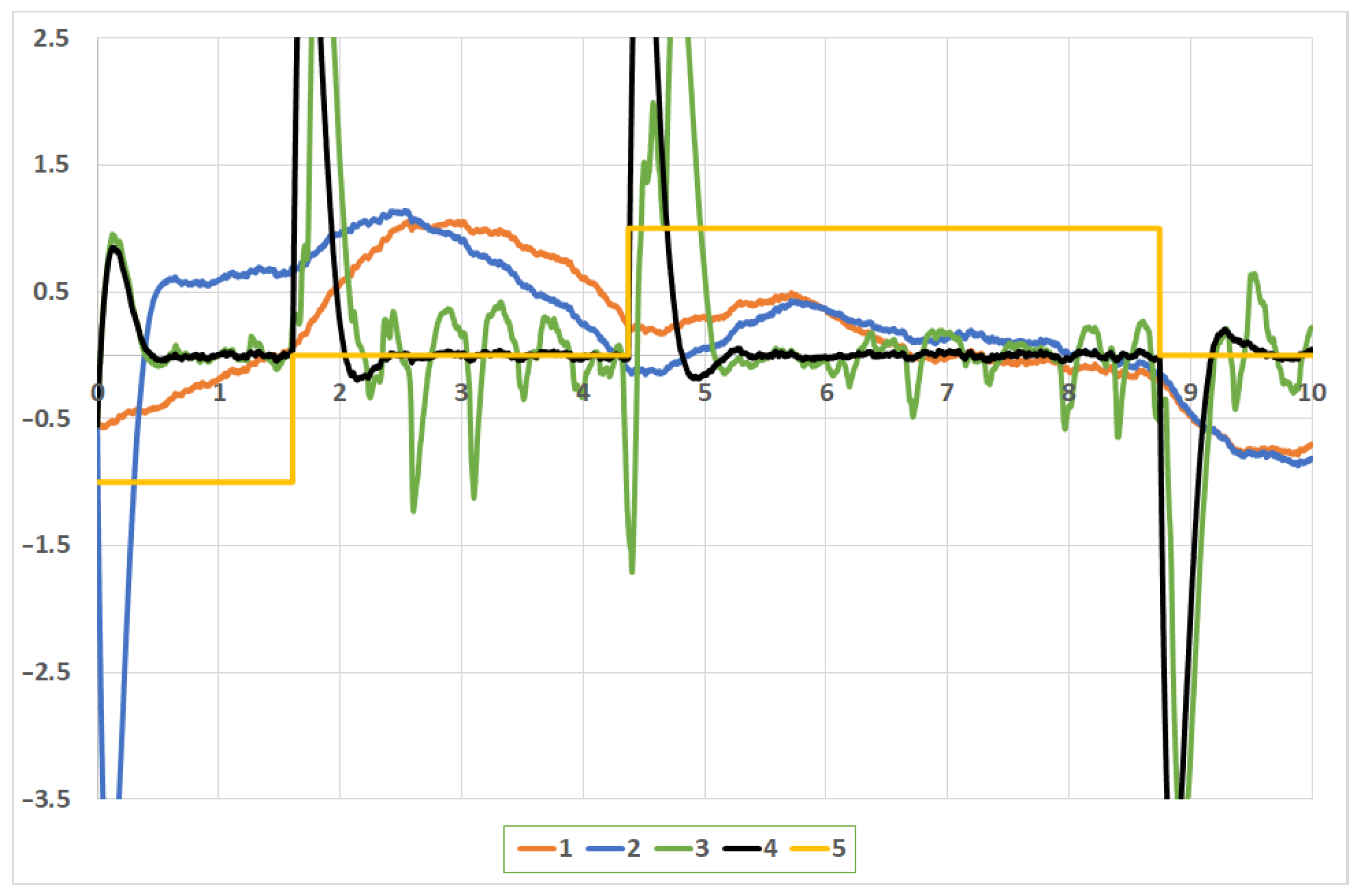
Figure 6 contains plots of the actuator velocity governed by various types of the assisting control:

• $v_t^{\left(0\right)}$ obtained under control $u_t^{\left(0\right)}$;
• $v_t^{me}$ obtained under control $u_t^{me}$;
• The optimal trajectory $v_t^{*}$ calculated for the optimal control $u_t^{*}$;
• The ”ideal” trajectory $v_t^{**}$ calculated for the control $u_t^{**}$.

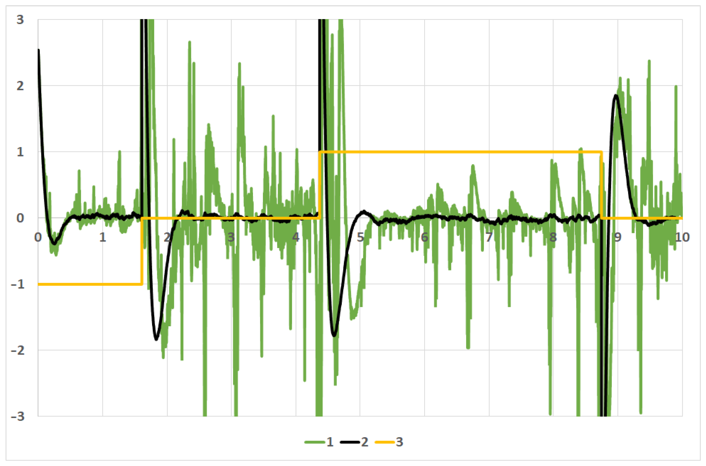
Finally, Figure 7 contains the following:

• The optimal control $u_t^{*}$;
• The “ideal” control $u_t^{**}$.

We also calculate objective values for various control types: $J\left({\left(U^{*}\right)}_0^T\right)=1.71$. Meanwhile, $J\left({\left(U^{\left(0\right)}\right)}_0^T\right)=8.65$ and $J\left({\left(U^{me}\right)}_0^T\right)=7.83$, i.e., the optimal assistance improves the actuator performance significantly. Additionally, we calculate the performance index for the “ideal” control: $J\left({\left(U^{**}\right)}_0^T\right)=1.29$, i.e., it does not demonstrate superiority in comparison with optimal control $U^{*}$.

7. Conclusions

The principal results of the paper are as follows: the derived explicit form (17) of the optimal control in the problem at hand and the fact that this optimal solution is indeed a feedback control, in which the key role is played by the solution of the auxiliary optimal filtering problem, i.e., conditional expectation $Y_t=E\left\{y_t|{\mathcal{F}}_t^Z\right\}$.

This provided grounds to formulate the main result, which is the separation theorem, generalizing the results of [29,30,31] to a general criterion (3). The fundamental difference between the classical LQG and the alternatives proposed in the referenced papers and the present research is that the transformed problem is not similar to the original one: the martingale representation of MJP (2) is replaced by a completely different object—the stochastic Ito equation with a Wiener process (9). Thus, the key to the solution turned out to be a unique property of the Wonham filter, which presents the MJP estimate given the indirect noisy observations in the form of the classical Ito equation with a Wiener process.

The obtained results admit the following interpretation and extensions. First, in the initial partially observable system, process $y_t$ can be treated as an unobservable system state; meanwhile, process $z_t$ plays the role of the controlled observable output. This point of view can be useful for various applications. Second, the obtained results remain valid in general if one complements the initial optimality criterion (3) by the additional terms ${\left|y_t-z_t\right|}^2$ for the output optimal tracking and by ${\left|u_t\right|}^2$ and ${\left|z_t\right|}^2$ for the optimal output/cost control. Third, the MJP $y_t$ can be replaced by any random process with a finite moment of the second order described by some nonlinear stochastic differential equation. In this case, the separation theorem is still correct, but coefficient $\beta$ in the optimal control is defined by some partial differential equation, and the optimal filtering estimate ${\widehat{y}}_t$ is described via the solution to the Kushner–Strtonovich or Duncan–Mortensen–Zakai equation. Fourth, if $y_t$ is an MJP, the diffusion coefficient ${\sigma }_t$ in (1) can be replaced by function $\sigma (t,y_t)$. In this manner, we extend the class dynamics by the systems with both the statistically uncertain piecewise constant drift and diffusion. All separation theorems and optimal control formulae remain valid. However, the solution to the optimal filtering problem is not expressed by the original Wonham filter but via its generalization [41,42].