Parameter Identification of Photovoltaic Models by Hybrid Adaptive JAYA Algorithm

Abstract

As one of the most promising forms of renewable energy, solar energy is increasingly deployed. The simulation and control of photovoltaic (PV) systems requires identification of their parameters. A Hybrid Adaptive algorithm based on JAYA and Differential Evolution (HAJAYADE) is developed to identify these parameters accurately and reliably. The HAJAYADE algorithm consists of adaptive JAYA, adaptive DE, and the chaotic perturbation method. Two adaptive coefficients are introduced in adaptive JAYA to balance the local and global search. In adaptive DE, the Rank/Best/1 mutation operator is put forward to boost the exploration and maintain the exploitation. The chaotic perturbation method is applied to reinforce the local search further. The HAJAYADE algorithm is employed to address the parameter identification of PV systems through five test cases, and the eight latest meta-heuristic algorithms are its opponents. The mean RMSE values of the HAJAYADE algorithm from five test cases are 9.8602 × 10⁻⁴, 9.8294 × 10⁻⁴, 2.4251 × 10⁻³, 1.7298 × 10⁻³, and 1.6601 × 10⁻². Consequently, HAJAYADE is proven to be an efficient and reliable algorithm and could be an alternative algorithm to identify the parameters of PV systems.

1. Introduction

Nowadays, governments and the public are more concerned about environmental protection and the energy crisis, meaning that the unsustainable energy structure dominated by fossil energy urgently needs to be adjusted. They have turned to renewable energy, which may be the main alternative to fossil fuels. Among various renewable energies, solar energy is one of the most promising energies as it is clean, renewable, green, etc. [1]. For solar energy, photovoltaic (PV) systems are commonly used because they can transform solar energy into electrical energy. It is reported that the market for PV systems has increased by as much as 50%, with more than 700,000 solar panels installed every day [2]. However, PV systems are often deployed in harsh environments, so that the utilization efficiency is greatly influenced. It is indispensable to assess the performance behavior of PV systems using models on the basis of observation data. Commonly used models are the single-diode model (SDM) and double-diode model (DDM). The performance of these models relies on the involved parameters. However, they are not available directly as they vary due to the harsh environments. Therefore, it is necessary to estimate the parameters of these models.

Identifying the parameters of these models can be defined as an optimized problem. There are two main approaches to solve the problem, i.e., the mathematical method and meta-heuristic algorithms. The former often tries to minimize a suitable function by imposing restrictions such as convexity and differentiability [3]. However, the problem is often nonlinear and multimodal, making the mathematical method ineffective and causing it to quickly fall into the local optimum [4]. Hence, various approaches are based on meta-heuristic algorithms.

Meta-heuristic algorithms are widely used to estimate the parameters of PV systems as they are simple, flexible, and derivation-free. These algorithms are developed based on the evolutionary concept, biological behavior, and physical phenomena. A teaching–learning optimization algorithm that simulates the learning and teaching process was combined with the artificial bee colony algorithm that forges the behavior of honey bees [2]. An oppositional teaching–learning algorithm was put forward to solve the problem. The opposition–learning technique was used to help the algorithm escape from the local optimum [5]. The multiple learning backtracking search optimization algorithm was realized for estimating the parameters, in which multi-updating strategies were developed to boost the diversity of the population [6]. An adaptive and chaotic grey wolf optimizer was designed to deal with the issue [7]. A multi-swarm spiral leader particle swarm optimization (PSO) algorithm was implemented to identify parameters. Several search mechanisms were used in the algorithm to achieve good performance [8]. The improved slime mould algorithm introduced Lévy flight (LF) and adaptive factors to attain the same aim [8]. In other work, an advanced slime mould algorithm was developed to solve three commercial PV models [9]. The Whippy Harris Hawks algorithm, as an extended version of Harris Hawks optimization, was designed to estimate the parameters of PV systems, and superior search capability was attained [10]. A robust and reliable approach on the basis of a stochastic fractal search algorithm was used to address the problem, in which three PV models were involved [11]. A hybrid algorithm based on the Rao algorithm and the chaotic map was developed and exhibited minor deviation when addressing the problem [12]. An improved marine predators algorithm using two different mutation strategies was proposed for the issue, and serial experiments achieved better results [13]. An extended gaining–sharing knowledge algorithm was applied to extract the parameters of PV systems, in which an adaptive mechanism was incorporated into the algorithm [14]. An adaptive differential evolution (DE) algorithm was developed to address the problem, and the experimental results from three PV models proved the efficiency of the algorithm [15]. An enhanced metaphor-free Gradient-based Optimizer Algorithm (GOA) was developed to cope with the issue [16]. An opposition-based GOA was also realized to identify the parameters of PV systems [17]. An effective and efficient solver called SFLBS was employed to tackle the problem [18]. Based on GOA, chaotic GOA was realized to derive PV systems’ parameters [19]. An ensemble multi-strategy-driven shuffled frog leading algorithm was developed to optimize the PV’s parameters to guarantee the optimal energy conversion [20].

These algorithms have attained remarkably good results when estimating the parameters of PV systems. However, it has to be pointed out that most of the above algorithms have to use additional parameters, except for the population size. The parameter settings greatly influence the performance of these algorithms. Setting the proper parameter values for a specific problem is still challenging. The parameter tuning is also a tedious task. Therefore, developing a competitive and advanced algorithm to extract the parameters of these models is still demanding work.

JAYA, developed by Rao [21], is a novel meta-heuristic algorithm. Its parameter-free nature makes the algorithm different from the conventional meta-heuristic algorithms. For instance, the genetic algorithm employs the crossover and mutation probabilities, PSO uses the inertia weight, etc. The algorithm attains the optimal solution by approaching the best solution and avoiding the worst solution. The algorithm’s structure is simple, and the algorithm is easy to implement. Therefore, the algorithm has also been used to solve problems in industrial applications [3,22,23,24,25,26,27,28,29,30]. For example, JAYA has been applied to solve the standard hybrid energy system [29]. It has been integrated with a branch and bound algorithm (BBA) to optimize the scheduling problem [30]. Various variants based on the JAYA algorithm have been proposed, and several variants based on JAYA have been employed to estimate the parameters of PV models. A comprehensive learning JAYA algorithm was developed by introducing the comprehensive learning mechanism to solve the parameters of three PV models [31]. An enhanced JAYA was developed to accurately and efficiently address the problem, in which three extensions were incorporated [32]. Performance-guided JAYA was offered, in which the promising search direction was controlled [4]. A logistic chaotic JAYA algorithm was realized and the algorithm used logistic chaotic map and mutation strategies to boost the population diversity [33]. An Improved JAYA (IJAYA) was realized by randomly selecting two mutation strategies. The proposed JAYA algorithm was used to address the problem [3]. Although these works have boosted the performance of JAYA, they also may demonstrate some deficiencies. For example, the two mutation strategies are randomly used in the IJAYA algorithm, without considering the quality of the solution. The search capability is limited when extracting the parameters of PV models [4] and these improvements are only based on JAYA, without considering the hybrid idea.

As demonstrated above, the aforementioned meta-heuristic algorithms have been successfully applied to solve the parameter identification of PV models [3,4,32,34,35]. However, these algorithms show different performances when attaining or approaching an optimal solution. Some have defects, such as lower robustness, premature convergence, and not exploiting the local information. It is necessary to design a competitive algorithm to address the problem. Meanwhile, these efforts seldom use the hybrid idea to create updating mechanisms, leading to limited improvements. Hybridization integrates the advantages of different algorithms to establish a hybrid algorithm while minimizing the substantial disadvantage. It is a common approach to boost the performance of evolutionary algorithms. An effective hybrid algorithm named whale optimization/DE algorithm was developed to estimate the parameters of PV models [36]. A hybrid GA-PSO algorithm was proposed to optimize the size of a house with PV panels, batteries, and wind turbines [37]. A hybrid algorithm using multiverse optimizer, equilibrium optimization, and moth flame optimization methods was implemented to tackle the optimal designs for wave energy converters [38]. A hybrid cooperative co-evolution algorithm was also developed [39]. In general, there are still shortcomings in the research on JAYA, which need to be improved by promoting the identification parameters of PV systems based on the hybrid idea.

In light of these observations, a Hybrid Adaptive JAYA and Differential Evolution (HAJAYADE) algorithm is developed. This is proposed based on the strengths and weaknesses of JAYA and DE. For JAYA, it is simple, while the search capacity is limited. Meanwhile, the adaptive JAYA position updating mechanism introduces two adaptive coefficients to boost the local and global search balance. The DE algorithm is flexible, and the search capacity depends on mutation strategies [40,41]. Among these mutation strategies of DE, Best/1 is commonly used with powerful exploitation and weak exploitation [42]. The Rank/Best/1 is put forward to enhance the exploration of the algorithm and maintain the exploitation by introducing the ranking information of individuals into the mutation strategy. To enhance the search capacity, the solutions obtained from the proposed HAJAYADE algorithm have been updated through three mutation strategies, the adaptive JAYA position updating mechanism, the Rank/Best/1 mutation strategy of DE algorithm, and the chaotic perturbation. The chaotic perturbation is widely used in JAYA variants and is adopted here to search around the best solution so that the exploitation can be further advanced [3,4]. The search capacity of the proposed HAJAYADE algorithm is greatly enhanced and used to solve the identification of PV parameters. The HAJAYADE algorithm is compared with eight meta-heuristic algorithms, the conventional JAYA and DE algorithms. A statistical test is performed to validate the performance of the proposed HAJAYADE algorithm. Therefore, the paper narrows the knowledge gap by the following contributions:

(1)

Two adaptive coefficients are introduced into JAYA to balance the local and global search so that an adaptive JAYA (AJAYA) is developed.

(2)

An adaptive DE algorithm is put forward by the novel Rank/Best/1 mutation operator, which considers the quality of the solution in the mutation stage.

(3)

A Hybrid Adaptive algorithm based on JAYA and Differential Evolution (HAJAYADE) is developed to identify the parameters of PV systems.

(4)

The HAJAYADE is proven to be an efficient and reliable algorithm compared with eight opponents.

The PV models are introduced and the objective functions are defined in Section 2. The JAYA and DE algorithms are introduced and the proposed HAJAYADE algorithm is elaborated in Section 3. The experiments and the analysis of the results are described in Section 4. The conclusions are made in Section 5.

2. PV Modeling Formation

There are several models to describe PV systems. Among these models, SDM and DDM are widely used in electrical engineering. In this section, SDM, DDM, and PV module models, based on SDM and DDM, are briefly introduced, and the objective function of the PV model is formatted.

2.1. Mathematical Model

(1)

Single-diode model (SDM)

SDM can precisely depict the static features of the solar cell. The model consists of a resistor to show the leakage current, and a serial resistor to describe the losses of the current. The model is demonstrated in [4].

The current $I_L$ can be computed as follows:

$$I_L=I_{ph}-I_d-I_{sh}$$

(1)

$$I_d=I_{sd}\times \left[\exp \left(\frac{q\times \left(V_L+R_s\times I_L\right)}{n\times k\times T}\right)-1\right]$$

(2)

$$I_{sh}=\frac{V_L+R_s\times I_L}{R_{sh}}$$

(3)

where $I_L$ is the current of the output, $I_{ph}$ is the current from the solar cell, $I_d$ is the current from the diode, which can be computed by Equation (2), $R_s$ and $R_{sh}$ are two resistors, $V_L$ is the output of the cell voltage, $I_{sd}$ is from the reverse saturation of the diode, $n$ is the feature factor of the diode, both $k=1.3806503\times {10}^{-23}\mathrm{J}/\mathrm{K}$ and $q=1.60217646\times {10}^{-19}\mathrm{C}$ are constants. The parameter $T$ is the absolute temperature of the cell. Equations (1)–(3) can be combined, and the output cell can be depicted as follows:

$$I_L=I_{ph}-I_{sd}\times \left[\exp \left(\frac{q\times \left(V_L+R_s\times I_L\right)}{n\times k\times T}\right)-1\right]-\frac{V_L+R_s\times I_L}{R_{sh}}$$

(4)

where five parameters $\left(I_{ph},I_{sd},R_s,R_{sh},n\right)$ are unknown and need to be estimated. These parameters have to be identified so that the performance of the solar cells can be fully measured. The problem can be addressed by optimization algorithms.

(2)

Double-diode model (DDM)

Different from the SDM, the DDM has double diodes. The DDM considers the influence of recombination current loss. Ref. [4] shows the circuit, and the output can be computed as follows:

$$\begin{array}{ll}{I}_L=I_{ph}-I_{d1}-& I_{d2}-I_{sh}\\ & =I_{ph}-I_{sd1}\times \left[\exp \left(\frac{q\times \left(V_L+R_s\times I_L\right)}{n_1\times k\times T}\right)-1\right]\\ & -I_{sd2}\times \left[\exp \left(\frac{q\times \left(V_L+R_s\times I_L\right)}{n_2\times k\times T}\right)-1\right]-\frac{V_L+R_s\times I_L}{R_{sh}}\end{array}$$

(5)

where $I_{sd1}$ and $I_{sd2}$ are the diffusion and saturation current, $n_1$ and $n_2$ are the diffusion diode and recombination diode ideal factor. There are seven parameters $\left(I_{ph},I_{sd1},I_{sd2},R_s,R_{sh},n_1,n_2\right)$ that need to be estimated.

(3)

PV module model

According to [4], the PV module model is built on a number of PV cells in parallel or/and in series. The module is based on the single-diode module model (SMM) and double-diode module model (DMM). The output current of the SMM is computed as follows:

$$\begin{array}{c}{I}_L=(I_{ph}-I_{sd}\times \left[\exp \left(\frac{q\times \left(V_L\times I_L/N_s+R_s\times I_L/N_p\right)}{n\times k\times T}\right)-1\right]\\ -\frac{V_L/N_s+R_s\times I_L/N_p}{R_{sh}})\times N_p\end{array}$$

(6)

where $N_p$ is the number of solar cells in parallel, and $N_s$ is the number of solar cells in series. Hence, five parameters $\left(I_{ph},I_{sd},R_s,R_{sh},n\right)$ need to be estimated.

2.2. Problem Formation

The parameters of the above models need to be estimated so that the performance of PV can be measured. Generally, the issue can be transformed into an optimization problem by minimizing the calculated and experimental data difference. The error can be defined by the following equations, in which Equations (7)–(9) are for SDM, DDM, and SMM, and $x$ is the set of unknown parameters to be evaluated.

$$\{\begin{array}{c}F\left(V_L,I_L,x\right)=I_{ph}-I_{sd}\times \left[\exp \left(\frac{q\times \left(V_L+R_s\times I_L\right)}{n\times k\times T}\right)-1\right]-\frac{V_L+R_s\times I_L}{R_{sh}}-I_L\\ x=\left\{I_{ph},I_{sd},R_s,R_{sh},n\right\} \end{array}$$

(7)

$$\{\begin{array}{c}F\left(V_L,I_L,x\right)=I_{ph}-I_{sd1}\times \left[\exp \left(\frac{q\times \left(V_L+R_s\times I_L\right)}{n_1\times k\times T}\right)-1\right]-\\ I_{sd2}\times \left[\exp \left(\frac{q\times \left(V_L+R_s\times I_L\right)}{n_2\times k\times T}\right)-1\right]-\frac{V_L+R_s\times I_L}{R_{sh}}-I_L\\ x=\left\{I_{ph},I_{sd1},I_{sd2},R_s,R_{sh},n_1,n_2\right\} \end{array}$$

(8)

$$\{\begin{array}{c}F\left(V_L,I_L,x\right)=(I_{ph}-I_{sd}\times \left[\exp \left(\frac{q\times \left(\frac{V_L\times I_L}{N_s}+R_s\times \frac{I_L}{N_p}\right)}{n\times k\times T}\right)-1\right]\\ -\frac{V_L/N_s+R_s\times I_L/N_p}{R_{sh}})\times N_p-I_L\\ x=\left\{I_{ph},I_{sd},R_s,R_{sh},n\right\} \end{array}$$

(9)

In previous studies, the root mean square error (RMSE) is employed as the objective function to measure the difference between simulated and experimental data [4]. If there are measurement errors, we can perform multiple measurements, and the mean result can be obtained and used as the experimental data. The measurement errors can be reduced. Minimizing the objective function is to search for the optimal solution $x$ in the specific range.

$$\mathrm{RMSE}\left(x\right)=\sqrt{\frac{1}{N}{\displaystyle \sum }_{k=1}^N{f}_k{\left(V_L,I_L,x\right)}^2}$$

(10)

where $N$ is the number of experimental data, and $x$ is the solution needed to be optimized.

3. Proposed HAYAJADE Algorithm Based on JAYA Algorithm and DE Algorithm

Both JAYA and DE are population-based evolutionary algorithms. In this section, two algorithms are briefly presented. Initialization is the first step for both algorithms. For a minimization problem, let $f\left(x\right)$ be the objective function with $D$-dimension ($j=1, 2,\dots ,D$), $x_{i,j}$ is the value of $jth$ dimension for $ith$ candidate solution and $x_i=\left(x_{i,1},x_{i,2},\dots ,x_{i,j},\dots ,x_{i,D}\right)$ is the $ith$ candidate solution’s position. The range of $x_{i,j}$ is between $L_j$ and $U_j$. The initial solution $x_{i,j}$ can be generated as follows:

$$x_{i,j}=L_j+\left(U_j-L_j\right)\times ran{d}_{i,j},j=1,2,\dots ,D$$

(11)

where $ran{d}_{i,j}$ is a random number between 0 and 1, $U_j$ and $L_j$ are upper and lower boundaries of the $jth$ dimension.

3.1. JAYA Algorithm

JAYA is a novel evolutionary algorithm compared with the DE algorithm. It was developed by Rao [21]. The algorithm can be employed to solve constrained and unconstrained problems. It is based on the idea that the solution should approach the best solution and avoid the worst solution when optimizing a specific problem. Unlike the conventional population-based evolutionary algorithms, JAYA is parameter-free, as it only has a common parameter, i.e., population size.

The best solution $x_{best}=\left\{x_{best,1},x_{best,2},\dots ,x_{best,D}\right\}$ has the minimization fitness value, while $x_{worst}=\left\{x_{worst,1},x_{worst,2},\dots ,x_{worst,D}\right\}$ has the maximization fitness value among the current solutions. Then, $x_{i,j}$ is updated by the following equation:

$$x_{i,j}^{\prime }=x_{i,j}+ran{d}_1\times \left(x_{best,j}-\left|x_{i,j}\right|\right)-ran{d}_2\times \left(x_{worst,j}-\left|x_{i,j}\right|\right)$$

(12)

where $ran{d}_1$ and $ran{d}_2$ are two random numbers between 0 and 1, $x_{worst,j}$ and $x_{best,j}$ are values of the $jth$ dimension for the worst and best solutions, $\left|x_{i,j}\right|$ is the absolute value of the $jth$ dimension for the $ith$ solution, $x_{i,j}^{\prime }$ and $x_{i,j}$ are the updated and the original values of the $jth$ dimension for the $ith$ solution. The term $x_{best,j}-\left|x_{i,j}\right|$ is used to denote the tendency towards the optimal solution, while the term $x_{worst,j}-\left|x_{i,j}\right|$ is applied to represent the tendency to avoid the worst solution.

If the generated individual $x_i^{\prime }$ is superior to the original individual $x_i$, the new individual $x_i^{\prime }$ will take the place of the original one. Otherwise, the original one is kept. The process can be mathematically presented as follows:

$$x_i=\{\begin{array}{c}{x}_i^{\prime }, if f\left(x_i^{\prime }\right)<f\left(x_i\right)\\ x_i, otherwise\end{array}$$

(13)

3.2. DE Algorithm

The DE algorithm is also a very simple and efficient population-based evolutionary algorithm that is older than the JAYA algorithm [40]. However, it is one of the most popular evolutionary algorithms due to its structure, real number encoding, and effectiveness [43]. The steps in the DE algorithm involve mutation, crossover, and selection.

There are many mutation operators in the DE algorithm. The mutation operator Best/1 is commonly used as follows:

$$v_i=x_{best}+F\times \left(x_{r_1}-x_{r_2}\right)$$

(14)

where $r_1$ and $r_2$ are randomly generated between 1 and the value of population size ($r_1\ne r_2\ne i$), $x_{best}$ is the optimal solution found so far, $v_i$ is the mutant vector, and $F$ is the scalar factor in the range of 0 and 1. The term $x_{r_1}-x_{r_2}$ is the difference vector.

The following step is crossover. It is used to exchange the information between the individual $x_i=\left\{x_{i,1},x_{i,2},\dots ,x_{i,j},\dots ,x_{i,D}\right\}$ and the mutant vector $v_i=\left\{v_{i,1},v_{i,2},\dots ,v_{i,j},\dots ,v_{i,D}\right\}$. The most commonly used crossover operator is defined as follows:

$$u_{i,j}=\{\begin{array}{c}{v}_{i,j} if rand\le CR or j=J_{rand}\\ x_{i,j} otherwise\end{array}$$

(15)

where $rand$ is a random number between 0 and 1, $CR$ is the crossover constant, which can be defined by the user, $J_{rand}$ is the integer in the range of 1 and $D$ to make use of the fact that $u_i$ at least has a component from $v_i$.

The last step is the same as the JAYA algorithm, which is the greedy selection. If the $u_i$ is superior to the $x_i$, the $x_i$ is replaced by $u_i$. Otherwise, $u_i$ is abandoned and $x_i$ is kept.

$$x_i=\{\begin{array}{c}{u}_i, if f\left(u_i\right)<f\left(x_i\right)\\ x_i, otherwise\end{array}$$

(16)

3.3. Hybrid Adaptive JAYA and DE (HAJAYADE)

For population-based meta-heuristic algorithms, it is necessary to realize a balance between exploitation and exploration. The exploration is to search as broadly as possible to identify the potential region, while the exploitation is to search around the potential region. In the early stage of evolution, the exploration is encouraged to scatter throughout the whole search space. At the later stage of evolution, exploitation is more necessary to approach the optimal solution.

For the JAYA algorithm, the main feature is its parameter-free nature, which makes it attractive [21]. The algorithm uses information from the best and worst solutions to search around the space. The single search strategy used in JAYA is to approach the best solution and avoid the worst solution. However, the single strategy may deteriorate the exploitation and exploration capabilities of the algorithm, which may lead to the local optimum.

In recent years, many improvements have been implemented to improve the performance of JAYA [3,4,32,34,35]. However, these efforts seldom use the hybrid idea to design updating mechanisms, leading to limited improvements as the hybrid is a common approach to boost the performance for most evolutionary algorithms [44]. If the feature of DE is reasonably integrated into the framework of JAYA, the exploitation can be significantly boosted as the capacity is superior for the Best/1 mutation strategy. Meanwhile, an adaptive approach is used to enhance the exploration, and balance the exploitation and exploration in the proposed algorithm. Lastly, a chaotic method is applied to boost the exploitation further [18]. Based on the observations, we developed a Hybrid Adaptive JAYA and DE algorithm (HAJAYADE). The algorithm consists of adaptive JAYA (AJAYA), adaptive DE, and adaptive chaotic perturbation.

3.3.1. Adaptive JAYA (AJAJA)

The conventional JAYA assigns the same priority to the best and the worst solutions. The best solution can be given more priority, while the worse solution can be assigned less priority so that the search direction can approach the potential region more quickly. Hence, two adaptive coefficients are introduced as follows:

$$w_1=\{\begin{array}{c}1 f\left(x_{best}\right)=0\\ \frac{Mean\left(f\left(x\right)\right)}{f\left(x_{best}\right)} f\left(x_{best}\right)\ne 0\end{array}$$

(17)

$$w_2=\{\begin{array}{c}1 f\left(x_{worst}\right)=0\\ \frac{Mean\left(f\left(x\right)\right)}{f\left(x_{worst}\right)} f\left(x_{worst}\right)\ne 0\end{array}$$

(18)

where $x_{best}$ and $x_{worst}$ are the best and worst solutions found so far, $f\left(x_{best}\right)$ and $f\left(x_{worst}\right)$ are their fitness values, and $Mean\left(f\left(x\right)\right)$ is the mean value of these fitness values. For a minimization problem, $w_1$ is greater than 1 while $w_2$ is less than 1. As the iteration increases, they approach 1, as shown in Figure 1.

Then, the two adaptive coefficients are introduced into Equation (19) as follows:

$$x_{i,j}^{\prime }=x_{i,j}+w_1\times ran{d}_1\times \left(x_{best,j}-\left|x_{i,j}\right|\right)-w_2\times ran{d}_2\times \left(x_{worst,j}-\left|x_{i,j}\right|\right)$$

(19)

At the beginning of the iteration, the differences among $f\left(x_{best}\right), f\left(x_{worst}\right),$ and $Mean\left(f\left(x\right)\right)$ are significant. $w_1$ is larger while $w_2$ is smaller. The search direction is directly towards the potential region. At the later stage of the iteration, the difference among the three values is slight. $w_1$ and $w_2$ are very close to 1. The $x_{best}$ and $x_{worst}$ are also close to each other. The local search can be implemented. Therefore, we introduce two coefficients $w_1$ and $w_2$ to balance exploration and exploitation. Their values depend on the fitness values of solutions and do not need to introduce any extra parameters.

3.3.2. Adaptive DE Algorithm

The performance of the DE algorithm mainly relies on the mutation operator. For Best/1, the exploitation is powerful while the exploration is weak. Searching around the best solution may deteriorate the exploration. To maintain the exploitation and improve the exploration, we propose the Rank/Best/1 mutation operator in Equation (20).

$$v_i=x_{best}+rand\times \left(x_{rank{r}_1}-x_{r_2}\right)$$

(20)

where $rank{r}_1$ is the integer in the range of 1 and population size, $rand$ is a random number in the range of 0 and 1 to take the place of the scalar factor $F$ so that the lesser parameter is introduced. We select $rank{r}_1$ depending on the fitness value of $f\left(x_{rank{r}_1}\right)$. Firstly, we sort solutions based on their fitness values in ascending order. Then, we assign the ranking values $ran{k}_i$ to each solution. The better the solution, the smaller the $ran{k}_i$ [45]. The selection probability $p_i$ can be computed as follows:

$$ran{k}_i=NP-i$$

(21)

$$p_i=\frac{ran{k}_i}{NP}$$

(22)

where $i$ is the rank index, $ran{k}_i$ is the rank value, and $p_i$ is the selection probability. The better the solution, the more the $p_i$.

For the conventional Best/1, $r_1$ and $r_2$ are randomly generated. The difference vector $x_{r_1}-x_{r_2}$ does not change significantly, especially at the early stage. The search range and exploration are limited. Different from Best/1, the $rank{r}_1$ is generated and selected depending on its corresponding $p_{rank{r}_1}$. We randomly generate a random number $rand$ in the range of 0 and 1. If $p_{rank{r}_1}>rand$, we accept the $rank{r}_1$. Otherwise, we have to regenerate the $rank{r}_1.$ As the unique generated mechanism is used, the difference vector $x_{rank{r}_1}-x_{r_2}$ changes significantly, especially at the early stage. The search range is fully extended, and the exploration is boosted. At the latter stage, the difference in the population is much smaller, so the difference vector $x_{rank{r}_1}-x_{r_2}$ changes slightly. The exploitation is realized. To avoid the local optimum, $r_2$ is randomly generated in the range of 1 and $NP$ without using the unique approach.

3.3.3. Adaptive Chaotic Method

Lastly, the adaptive chaotic method is applied to improve the exploitation of the algorithm further. The chaotic approach has been proven valuable and successful in many evolutionary algorithms [3,4]. The method is used to explore the best solution, and a logistic map is a useful approach in many experiments of JAYA. Therefore, it is also adopted as follows:

$$z_k=\{\begin{array}{c}rand k=1\\ 4\times z_{k-1}\times \left(2\times z_{k-1}-1\right) k>1\end{array}$$

(23)

where $k$ is the index of iteration. When $k=1$, $z_k$ is randomly generated between 0 and 1. $z_k$ is used as a perturbation to the best solution.

$$x_j^{*}=\{\begin{array}{c}{x}_{best,j} otherwise\\ x_{best,j}+rand\times \left(2\times z_k-1\right) if rand<1-FES/FE{S}_{max}\end{array}$$

(24)

where $x_{best,j}$ is the value of the $jth$ dimension for $x_{best}$, $z_k$ is the value of $kth$ chaotic, $FES$ is the number of function evaluation, $FE{S}_{max}$ is the maximal function evaluation. At the early stage, the $FES$ is small and the condition $rand<1-FES/FE{S}_{max}$ is met more frequently; more chaotic perturbation is used to generate solutions around the $x_{best}$. At the later stage, with the increasing of $FES$, it is difficult to satisfy the condition $rand<1-FES/FE{S}_{max}$. $x_{best}$ is very close to the optimal solution, and more perturbation is unnecessary. If the solution $x_{}^{*}$ is superior to the worst solution, $x_{}^{*}$ will take the place of the solution. Otherwise, the solution $x_{}^{*}$ is discarded.

3.3.4. Framework of HAJAYADE

The proposed HAJAYADE algorithm is mainly based on JAYA and DE. Therefore, we use two populations for the two algorithms. By the greedy selection, the two populations form a single population. The flowchart of HAJAYADE is presented in Figure 2, and the pseudo-code of HAJAYADE is shown as follows (Algorithm 1).

Algorithm 1: HAJAYADE
Input:	$\mathrm{The}\mathrm{population}\mathrm{size}:NP$$;\mathrm{the}\mathrm{maximal}\mathrm{function}\mathrm{evaluation}(FE{S}_{max}$$);\mathrm{crossover}\mathrm{constant}CR$
Output:	The optimal solution
1	$\mathrm{Generate}\mathrm{initial}\mathrm{population}p$ by Equation (11)
2	Evaluate the fitness value of population p
3	$FES=NP;$
4	$\mathrm{While}(FES<FE{S}_{max}$)
5	$\mathrm{Identify}\mathrm{the}\mathrm{best}\mathrm{solution}{x}_{best}$$\mathrm{and}\mathrm{its}\mathrm{corresponding}\mathrm{fitness}\mathrm{value}f\left(x_{best}\right)$
6	$\mathrm{Identify}\mathrm{the}\mathrm{worst}\mathrm{solution}{x}_{worst }$$\mathrm{and}\mathrm{its}\mathrm{corresponding}\mathrm{fitness}\mathrm{value}f\left(x_{worst}\right)$
7	$\mathrm{Calculate}\mathrm{the}\mathrm{adaptive}\mathrm{parameters}{w}_1$$\mathrm{and}{w}_2$ by Equations (17) and (18)
8	$\mathrm{for}i=1:NP$
9	Update the population p$\mathrm{by}\mathrm{Equation}\left(19\right)\mathrm{and}\mathrm{generate}\mathrm{the}\mathrm{trial}\mathrm{vector}{x}_i^{\prime }$
10	end
11	$\mathrm{Compute}\mathrm{the}\mathrm{selection}\mathrm{probability}{p}_i$ according to Equation (22)
12	$\mathrm{for}i=1:NP$
13	$\mathrm{Generate}\mathrm{a}rand$ in the range of 0 and 1
14	$\mathrm{Randomly}\mathrm{select}\mathrm{an}\mathrm{integer}rank{r}_1$$\mathrm{in}\mathrm{the}\mathrm{range}\mathrm{of}1\mathrm{and}NP$
15	$\mathrm{While}(rand>p\left(rank{r}_1\right)||i==rank{r}_1$)
16	$\mathrm{Randomly}\mathrm{select}\mathrm{an}\mathrm{integer}\mathrm{rankr}1\mathrm{in}\mathrm{the}\mathrm{range}\mathrm{of}1\mathrm{and}NP$
17	end
18	$\mathrm{Randomly}\mathrm{select}\mathrm{an}\mathrm{integer}{r}_2$$\mathrm{in}\mathrm{the}\mathrm{range}\mathrm{of}1\mathrm{and}NP$
19	$\mathrm{While}(i==r_2||rank{r}_1==r_2$)
20	$\mathrm{Randomly}\mathrm{select}\mathrm{an}\mathrm{integer}{r}_2$$\mathrm{in}\mathrm{the}\mathrm{range}\mathrm{of}1\mathrm{and}NP$
21	end
22	$\mathrm{Generate}\mathrm{the}\mathrm{mutant}\mathrm{vector}{u}_i$ by Equation (20)
23	end
24	$\mathrm{for}i=1:NP$
25	$\mathrm{Generate}\mathrm{the}\mathrm{trial}\mathrm{vector}{v}_i$ by Equation (15)
26	end
27	$\mathrm{for}i=1:NP$
28	$\mathrm{Evaluate}\mathrm{the}\mathrm{fitness}\mathrm{value}\mathrm{of}{x}_i^{\prime }$$\mathrm{and}{v}_i$ respectively
29	$\mathrm{if}(f\left(x_i^{\prime }\right)<f\left(x_i\right)$)
30	$x_i=x_i^{\prime }; f\left(x_i\right)=f\left(x_i^{\prime }\right);$
31	end
32	$\mathrm{if}(f\left(v_i\right)<f\left(x_i\right)$)
33	$x_i=v_i; f\left(x_i\right)=f\left(v_i\right);$
34	end
35	$FES=FES+2;$
36	end
37	$\mathrm{Identify}\mathrm{the}\mathrm{best}\mathrm{solution}{x}_{best}$$\mathrm{and}\mathrm{the}\mathrm{worst}\mathrm{solution}{x}_{worst}$
38	$\mathrm{Use}\mathrm{the}\mathrm{chaotic}\mathrm{perturbation}\mathrm{to}\mathrm{generate}\mathrm{the}\mathrm{solution}{x}_{}^{*}$ by Equation (24)
39	$\mathrm{if}(f\left(x_{}^{*}\right)<f\left(x_{worst}\right))$
40	$x_{worst}=x_{}^{*};f\left(x_{}^{*}\right)=f\left(x_{worst}\right);$
41	end
42	$FES=FES+1;$
43	end
44	$\mathrm{Output}\mathrm{the}\mathrm{optimal}\mathrm{solution}{x}_{best}$$\mathrm{and}\mathrm{its}\mathrm{corresponding}\mathrm{fitness}f\left(x_{best}\right)$.

3.3.5. Complexity of the Proposed HAJAYADE Algorithm

The complexity of the HAYAYADE is discussed as follows. Let the population size be $NP$ and the dimension of the problem be $D$. Identifying the best and worst solutions, computing the mean fitness value demands $O\left(NP\right)$. Updating the position of population needs $O\left(NP\times D\right)$. Ranking solutions in the population requires $O\left(N\times Plog\left(NP\right)\right)$. The mutant process requires $O\left(NP\right)$. The crossover operator demands $O\left(NP\times D\right)$. The greedy selection for the hybrid algorithm requires $O\left(NP\right)$. The chaotic operator requires $O\left(D\right)$. Therefore, the total complexity of the proposed HAJAYADE algorithm needs $O\left(NP+NP\times D+NP\times log\left(NP\right)+NP+NP\times D+D\right)$. As the $log\left(NP\right)$ is often smaller than $D$, the complexity of the proposed HAJAYADE algorithm is $O\left(NP\times D\right)$.

4. Experimental Results and Analysis

The performance of the proposed HAJAYADE algorithm is used to estimate the parameters of PV models, including the SDM, DDM, and SMM. The current–voltage data are from reference [46]. They are widely employed to test diverse techniques developed to estimate the parameters of PV models. The data of SDM contain 26 groups of current and voltage under $1000\mathrm{W}/{\mathrm{m}}^2$ at $33°\mathrm{C}$, which is the RTC France Si cell. The DDM is measured by 57 silicon. The SMM includes the Photowatt-PWP201 PV model, STM6-40/36 PV model, STP6-120/36 PV model. The temperatures at the three PV models are $45°\mathrm{C},51°\mathrm{C},\mathrm{and}55°\mathrm{C}$ [32]. For the five problems, the range of parameters is listed in

Table 1. Ranges of parameters.

Parameter	SDM/DDM		Photowatt-PWP201		STM6-40/36		STP6-120/36
	Upper	Lower	Upper	Lower	Upper	Lower	Upper	Lower
$I_{ph}\left(A\right)$	1	0	2	0	2	0	8	0
$I_{sd},I_{sd1},I_{sd2}\left(\mu A\right)$	1	0	50	0	50	0	50	0
$n,n_1,n_2$	2	1	50	1	60	1	50	1
$R_s\left(\mathsf{\Omega }\right)$	0.5	0	2	0	0.36	0	0.36	0
$R_p\left(\mathsf{\Omega }\right)$	100	0	2000	0	1000	0	1500	0

.

To test the performance of the proposed HAJAYADE algorithm, some of the latest algorithms and their variants are used as its opponents, including GWO [47], CMAES [48], TLABC [2], TAPSO [49], MLBSA [6], GOTLBO [5], PGJAYA [4], and IJAYA [3]. GWO is a novel swarm intelligent algorithm proposed by Mirjalili et al. [47]. The self-adaptation of the mutation distribution is adopted in the CMAES algorithm to boost the local and global search [48]. TLABC is a hybrid algorithm based on TLBO and ABC, with the purpose of enhancing the reliability and accuracy of meta-heuristic algorithms [2]. In TAPSO, three archives are used to design an efficient learning model and select proper exemplars [49]. In MLBSA, a fraction of individuals learn from the elite solution, while the remaining individuals learn from the historical population and current population to balance the exploration and exploitation [6]. In GOTLBO, a generalized opposition-based learning technique is integrated into basic TLBO to enhance the convergence [5]. In the PGJAYA algorithm, each individual can adaptively select mutation strategies depending on its selection probability [4]. In IJAYA, an adaptive coefficient and an experience-based mutation operator are introduced to boost the diversity of the population and enhance the exploration [3].

The main parameters of the above nine algorithms are listed in

Table 2. Parameter values of ten algorithms.

Algorithm	Parameters
GWO	$\overrightarrow{a}$$\mathrm{linearly}\mathrm{decreases}\mathrm{from}2\mathrm{to}0;NP=20$
CMAES	$\sigma =0.25,NP=20$
TLABC	$limit=200,F=rand\left(0,1\right);NP=50$
TAPSO	$w=0.7298,p_c=0.5,p_m=0.02,NP=20$
MLBSA	$NP=50$
GOTLBO	$NP=50,J_r=0.3$
PGJAYA	$NP=20$
IJAYA	$NP=20$
HAJAYADE	$NP=20;C_r=0.5$

. These parameters are mainly based on their original references so that the best performances of these algorithms can be guaranteed. The maximal function evaluations are set to 50,000. Each algorithm runs thirty times independently, and the statistical results are obtained. These algorithms run on a PC with a memory of 8 GB, primary frequency of 3.4 GHz, Win 10 OS, and Matlab R2020a.

4.1. Results and Analysis

(1)

Results of SDM

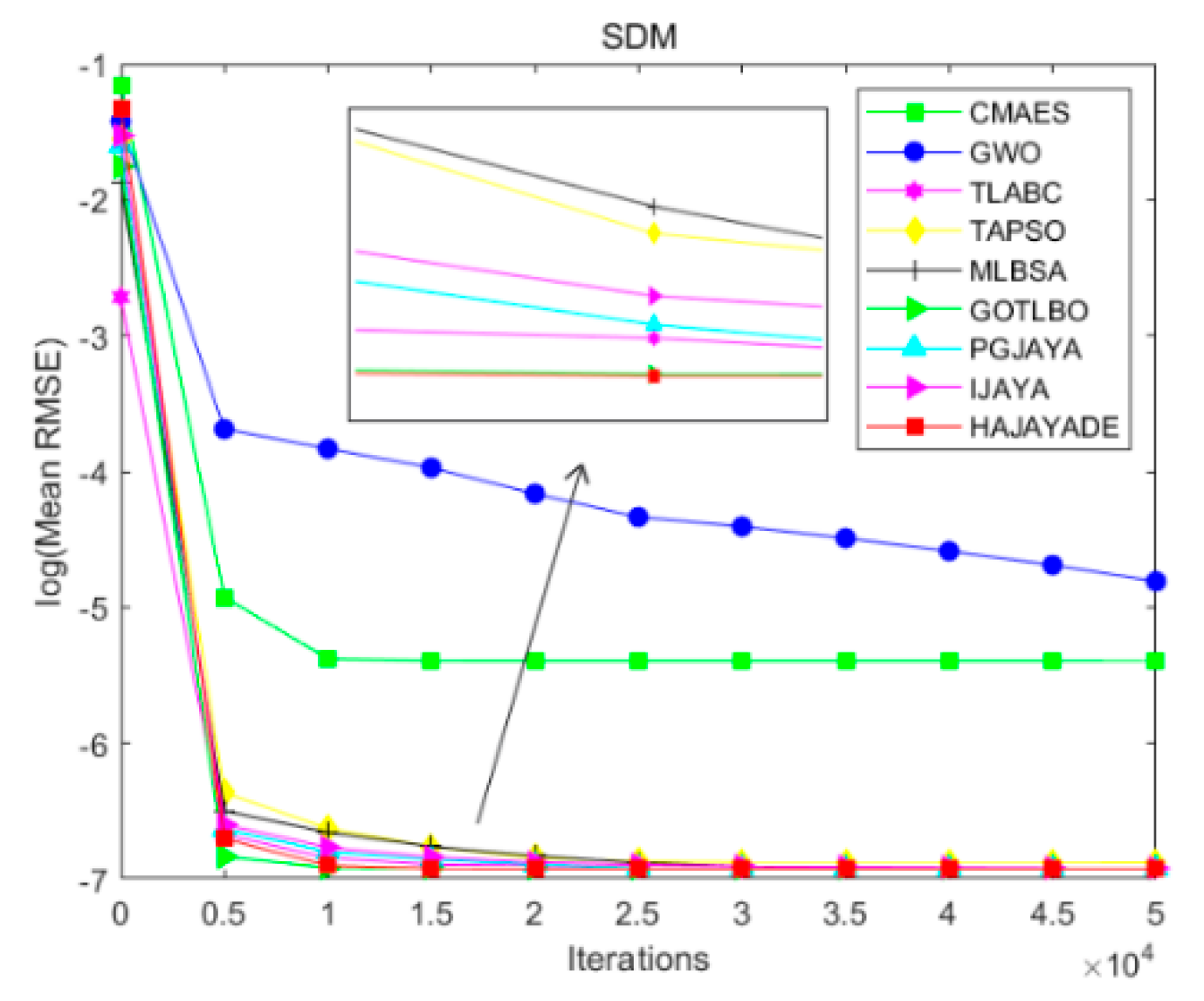
For the SDM, i.e., the RTC France Si cell, the statistical results involving the maximal, mean, minimal, and the standard deviation values of RMSE from the above nine algorithms, i.e., GWO, CMAES, TLABC, TAPSO, MLBSA, GOTLBO, PGJAYA, IJAYA, and HAJAYADE, are listed in

Table 3. Statistical results from nine algorithms for the SDM problem.

Algorithm	Min	Mean	Max	Std
CMAES	2.4203 × 10−³	4.501 × 10−³	9.7738 × 10−³	2.0983 × 10−³
GWO	1.0023 × 10−³	8.1335 × 10−³	4.4315 × 10−2	1.3204 × 10−2
TLABC	9.8602 × 10−4	9.9218 × 10−4	1.0317 × 10−³	1.1679 × 10−5
TAPSO	9.8602 × 10−4	1.0267 × 10−³	2.2063 × 10−³	2.228 × 10−4
MLBSA	9.8602 × 10−4	9.8602 × 10−4	9.8604 × 10−4	2.7152 × 10−9
GOTLBO	9.8602 × 10−4	1.01 × 10−³	1.3865 × 10−³	9.01 × 10−5
PGJAYA	9.8602 × 10−4	9.8602 × 10−4	9.8607 × 10−4	7.8692 × 10−9
IJAYA	9.8625 × 10−4	9.8924 × 10−4	9.9869 × 10−4	2.8943 × 10−6
HAJAYADE	9.8602 × 10−4	9.8602 × 10−4	9.8602 × 10−4	0

. In terms of the minimal value, most algorithms except GWO, CMAES, and IJAYA are the best. Only three algorithms, i.e., MLBSA, PGJAYA, and HAJAYADE, can obtain the best value in terms of the mean value. However, only the proposed HAJAYADE algorithm has the lowest maximal value. Therefore, the proposed HAYAJADE algorithm is the best one for the SDM. The convergence curves of the nine algorithms are plotted in Figure 3. It can be noticed that the convergence speed of GWO and CMAES is lower compared with the remaining algorithms. When the convergence curves are magnified, it can be observed that the convergence speed of these algorithms is also different, in which the proposed HAJAYADE algorithm is the fastest. The best solutions obtained from 30 runs for each algorithm are listed in

Table 4. Optimal solutions obtained from nine algorithms for SDM.

Algorithm	${\mathit{I}}_{\mathit{p}\mathit{h}}$	${\mathit{I}}_{\mathit{s}\mathit{d}}$	${\mathit{R}}_{\mathit{s}}$	${\mathit{R}}_{\mathit{s}\mathit{h}}$	$\mathit{n}$	RMSE
CMAES	0.76076	0.9522	0.031301	95.9066	1.5988	2.4203 × 10−³
GWO	0.76093	0.32791	0.03631	51.4854	1.4828	1.0023 × 10−³
TLABC	0.76078	0.32302	0.036377	53.7185	1.4812	9.8602 × 10−4
TAPSO	0.76078	0.32302	0.036377	53.7185	1.4812	9.8602 × 10−4
MLBSA	0.76078	0.32302	0.036377	53.7185	1.4812	9.8602 × 10−4
GOTLBO	0.76078	0.32302	0.036377	53.7185	1.4812	9.8602 × 10−4
PGJAYA	0.76078	0.32302	0.036377	53.7186	1.4812	9.8602× 10−4
IJAYA	0.76074	0.32302	0.036382	54.0089	1.4811	9.8625 × 10−4
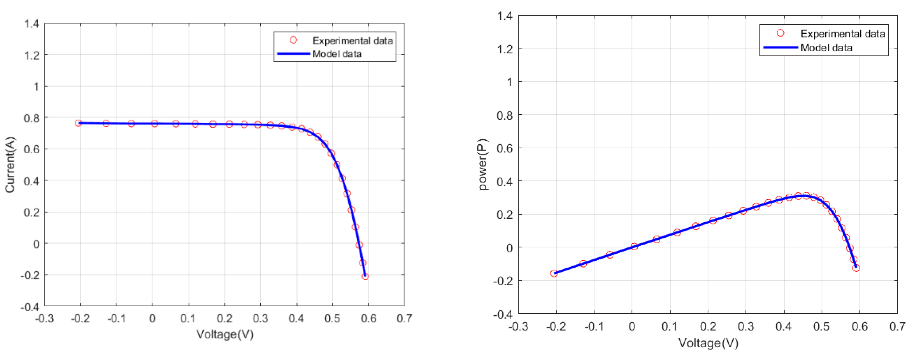
HAJAYADE	0.76078	0.32302	0.036377	53.7185	1.4812	9.8602× 10−4

. To validate the quality of the results obtained from the proposed HAJAYADE algorithm, the best-estimated values are employed to establish the relationship between the current and voltage in Figure 4. The experimental data are highly consistent with the calculated data. The figure further validates the effectiveness of the proposed HAJAYADE algorithm.

(2)

Results on the DDM

For the DDM, seven parameters need to be optimized, and the dimension is more than the SDM. The results from the above nine algorithms are revealed in

Table 5. Statistical results from nine algorithms for the DDM.

Algorithm	Min	Mean	Max	Std
CMAES	9.9015 × 10−4	3.2883 × 10−3	6.9683 × 10−3	1.8499 × 10−3
GWO	1.1429 × 10−3	9.6965 × 10−3	3.8045 × 10−2	1.2305 × 10−2
TLABC	9.8407 × 10−4	1.0616 × 10−3	1.4496 × 10−3	1.2359 × 10−4
TAPSO	9.8269 × 10−4	1.2853 × 10−3	2.3508 × 10−3	4.1093 × 10−4
MLBSA	9.8285 × 10−4	9.856 × 10−4	9.8778 × 10−4	9.3682 × 10−7
GOTLBO	9.8299 × 10−4	1.0303 × 10−3	1.4242 × 10−3	1.0111 × 10−4
PGJAYA	9.8298 × 10−4	9.8624 × 10−4	9.9773 × 10−4	2.9021 × 10−6
IJAYA	9.8631 × 10−4	1.0107 × 10−3	1.182 × 10−3	4.704 × 10−5
HAJAYADE	9.8294 × 10−4	9.8641 × 10−4	9.96 × 10−4	2.8534 × 10−6

, in which HAJAYADE has attained the best results in terms of the minimal (9.8294 × 10⁻⁴), mean (9.8641 × 10⁻⁴), and maximal value (9.96 × 10⁻⁴). The difference among these statistical results of the proposed HAJAYADE algorithm is tiny, indicating that the proposed HAYAJADE algorithm is robust. The result of PGJAYA is second only to the proposed HAJAYADE algorithm, ranking second. GWO has obtained the worst result as the algorithm only uses the top three wolves to guide the search direction. The exploration is limited, and the algorithm is easily trapped into the local optimum. The standard deviation of the algorithm is the largest, which indicates that GWO is less robust. The reason behind the superior performance is that the proposed HAJAYADE algorithm uses the hybrid mechanism, which boosts exploration and exploitation. The excellent performance can also be measured by convergence curves, in which the log (mean RMSE) is used as the value of the $y$-axis so that the difference among the nine algorithms is apparent. The convergence speed of the proposed HAJAYADE algorithm is much faster according to Figure 5. The best results attained from these algorithms are listed in

Table 6. Optimal solutions obtained from nine algorithms for DDM.

Algorithm	${\mathit{I}}_{\mathit{p}\mathit{h}}$	${\mathit{I}}_{\mathit{s}\mathit{d}1}$	${\mathit{R}}_{\mathit{s}}$	${\mathit{R}}_{\mathit{s}\mathit{h}}$	${\mathit{n}}_1$	${\mathit{I}}_{\mathit{s}\mathit{d}2}$	${\mathit{n}}_2$	RMSE
CMAES	0.76062	0.26941	0.036502	56.3321	1.4674	0.1659	1.7803	9.9015 × 10−4
GWO	0.76106	0.89499	0.036962	48.1939	1.3866	0.6471	1.729	1.1429 × 10−3
TLABC	0.76079	0.38772	0.036647	54.6552	1.8584	0.232	1.4546	9.8407 × 10−4
TAPSO	0.76079	0.67827	0.036741	54.9983	1.9987	0.23154	1.4529	9.8269 × 10−4
MLBSA	0.76078	0.5284	0.036623	54.9649	1.9978	0.25212	1.4602	9.8285 × 10−4
GOTLBO	0.76078	0.25815	0.036604	54.8163	1.4622	0.48047	1.9987	9.8299 × 10−4
PGJAYA	0.76078	0.25828	0.036598	54.8875	1.4622	0.48583	1.461	9.8298 × 10−4
IJAYA	0.76082	0.29722	0.036558	54.0126	1.8502	0.25073	1.461	9.8631 × 10−4
HAJAYADE	0.76078	0.49872	0.036602	54.9059	1.9992	0.25657	1.4617	9.8294 × 10−4

, and the result of the proposed HAJAYADE algorithm is used to construct the model. The experimental and calculated data from the proposed HAJAYADE algorithm are plotted in Figure 6. It is evident that the two groups’ data are in superior accordance.

(3)

Results on PV models

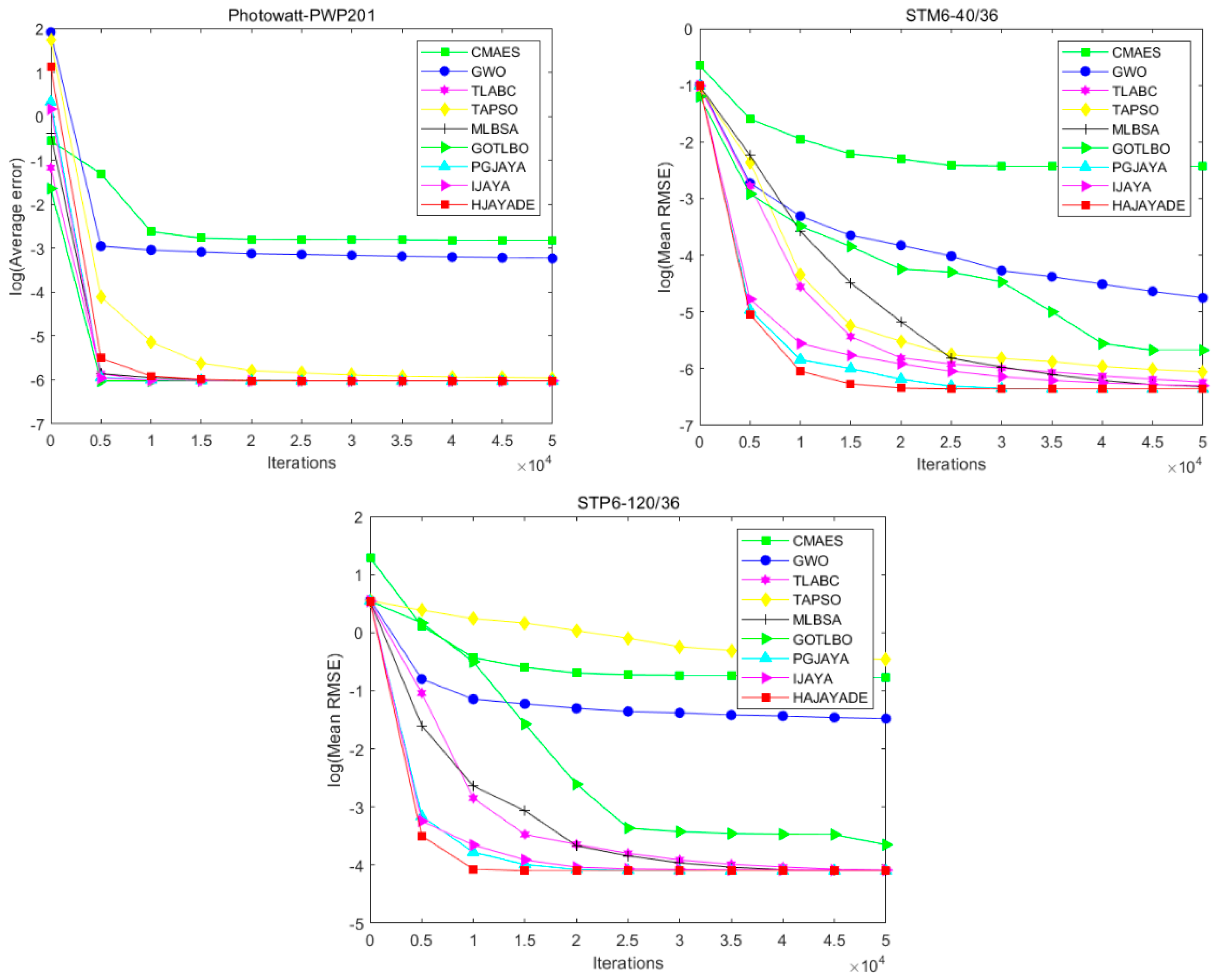
There are three PV models, the Photowatt-PWP201, the STM6-40/36, and the STP6-120/36. It is necessary to optimize five parameters. The above nine algorithms are used to identify these five parameters. The statistical results of the three groups are listed in

Table 7. Statistical results from nine algorithms for three PV models.

Model	Algorithm	Min	Mean	Max	Std
Photowatt-PWP201	CMAES	4.9842 × 10−3	5.957 × 10−2	2.5934 × 10−1	7.5656 × 10−2
	GWO	2.6039 × 10−3	3.9456 × 10−2	2.7431 × 10−1	9.368 × 10−2
	TLABC	2.4251 × 10−3	2.4266 × 10−3	2.4496 × 10−3	5.7303 × 10−6
	TAPSO	2.4251 × 10−3	2.5928 × 10−3	4.1483 × 10−3	3.8109 × 10−4
	MLBSA	2.4251 × 10−3	2.4251 × 10−3	2.4251 × 10−3	4.9687 × 10−10
	GOTLBO	2.4251 × 10−3	2.427 × 10−3	2.4621 × 10−3	7.5384 × 10−6
	PGJAYA	2.4251 × 10−3	2.4251 × 10−3	2.426 × 10−3	1.7877 × 10−7
	IJAYA	2.4251 × 10−3	2.427 × 10−3	2.4385 × 10−3	2.8147 × 10−6
	HAJAYADE	2.4251 × 10−3	2.4251 × 10−3	2.4251 × 10−3	3.2215 × 10−15
STM6-40/36	CMAES	1.9343 × 10−3	8.8897 × 10−2	1.613 × 10−1	5.1349 × 10−2
	GWO	4.8387 × 10−3	8.6059 × 10−3	1.7596 × 10−2	3.3055 × 10−3
	TLABC	1.7298 × 10−3	1.9398 × 10−3	2.6262 × 10−3	2.2746 × 10−4
	TAPSO	1.7298 × 10−3	2.3263 × 10−3	1.0566 × 10−2	1.5873 × 10−3
	MLBSA	1.7298 × 10−3	1.8 × 10−3	3.7038 × 10−3	3.5966 × 10−4
	GOTLBO	1.7298 × 10−3	3.4321 × 10−3	2.1722 × 10−2	3.5876 × 10−3
	PGJAYA	1.7298 × 10−3	1.7302 × 10−3	1.7376 × 10−3	1.4416 × 10−6
	IJAYA	1.7345 × 10−3	1.8305 × 10−3	2.221 × 10−3	1.2044 × 10−4
	HAJAYADE	1.7298 × 10−3	1.7298 × 10−3	1.7298 × 10−3	3.6569 × 10−16
STP6-120/36	CMAES	1.6612 × 10−2	5.2725 × 10−1	1.4131	6.0591 × 10−1
	GWO	1.733 × 10−2	2.2768 × 10−1	1.4131	4.1976 × 10−1
	TLABC	1.6601 × 10−2	1.6775 × 10−2	1.8269 × 10−2	3.3454 × 10−4
	TAPSO	5.7763 × 10−2	6.2436 × 10−1	1.299	3.7049 × 10−1
	MLBSA	1.6601 × 10−2	1.6627 × 10−2	1.6786 × 10−2	4.1209 × 10−5
	GOTLBO	1.6605 × 10−2	2.2226 × 10−2	5.9712 × 10−2	9.5158 × 10−3
	PGJAYA	1.6601 × 10−2	1.6609 × 10−2	1.6722 × 10−2	2.7355 × 10−5
	IJAYA	1.6733 × 10−2	1.6813 × 10−2	1.691 × 10−2	4.1722 × 10−5
	HAJAYADE	1.6601 × 10−2	1.6601 × 10−2	1.6606 × 10−2	9.2421 × 10−7

. GWO and CMAES have attained inferior results for the three groups. Except for the two algorithms, TAPSO has obtained worse results for both Photowatt-PWP201 (2.5928 × 10⁻³) and STP6-120/36 (6.2436 × 10⁻¹), and GOTLBO is inferior for STM6-40/36 in terms of the mean value (3.4321 × 10⁻³). On the contrary, regarding the three JAYA variants, the performances of PGJAYA, IJAYA, and HAJAYADE are better. In more detail, PGJAYA and HAJAYADE have attained the best results for Photowatt-PWP201. The performances of HAJAYADE are more robust compared with PGJAYA and IJAYA. Thus, it is the best one among the nine algorithms.

The solutions attained from these algorithms are presented in

Table 8. Optimal solutions attained from nine algorithms for three PV models.

Model	Algorithm	${\mathit{I}}_{\mathit{p}\mathit{h}}$	${\mathit{I}}_{\mathit{s}\mathit{d}}$	${\mathit{R}}_{\mathit{s}}$	${\mathit{R}}_{\mathit{s}\mathit{h}}$	$\mathit{n}$	RMSE
Photowatt-PWP201	CMAES	1.0467	0.19815	1.2319	316.3977	46.6264	4.9842 × 10−3
	GWO	1.0287	0.48801	1.1664	1544.616	49.969	2.6039 × 10−3
	TLABC	1.0305	0.34823	1.2013	981.9822	48.6428	2.4251 × 10−3
	TAPSO	1.0305	0.34823	1.2013	981.9824	48.6428	2.4251 × 10−3
	MLBSA	1.0305	0.34823	1.2013	981.9823	48.6428	2.4251 × 10−3
	GOTLBO	1.0305	0.34823	1.2013	981.9823	48.6428	2.4251 × 10−3
	PGJAYA	1.0305	0.34823	1.2013	981.992	48.6429	2.4251 × 10−3
	IJAYA	1.0305	0.34864	1.2011	982.0576	48.6474	2.4251 × 10−3
	HAJAYADE	1.0305	0.34823	1.2013	981.9824	48.6428	2.4251 × 10−3
STM6-40/36	CMAES	7.4755	2.2665	0.0046056	17.8598	1.2576	1.6612 × 10−2
	GWO	7.4664	3.389	0.0044212	1052.2704	1.292	1.733 × 10−2
	TLABC	7.4725	2.335	0.0045946	22.2199	1.2601	1.6601 × 10−2
	TAPSO	7.4811	27.857	0.0028127	809.038	1.5075	5.7763 × 10−2
	MLBSA	7.4725	2.335	0.0045946	22.2202	1.2601	1.6601 × 10−2
	GOTLBO	7.4741	2.2787	0.0046047	19.572	1.2581	1.6605 × 10−2
	PGJAYA	7.4725	2.3351	0.0045946	22.2253	1.2601	1.6601 × 10−2
	IJAYA	7.4697	2.5505	0.0045678	40.1402	1.2675	1.6733 × 10−2
	HAJAYADE	7.4725	2.3351	0.0045946	22.2199	1.2601	1.6601 × 10−2
STP6-120/36	CMAES	7.4755	2.2665	0.0046056	17.8598	1.2576	1.6612 × 10−2
	GWO	7.4664	3.389	0.0044212	1052.2704	1.292	1.733 × 10−2
	TLABC	7.4725	2.335	0.0045946	22.2199	1.2601	1.6601 × 10−2
	TAPSO	7.4811	27.857	0.0028127	809.038	1.5075	5.7763 × 10−2
	MLBSA	7.4725	2.335	0.0045946	22.2202	1.2601	1.6601 × 10−2
	GOTLBO	7.4741	2.2787	0.0046047	19.572	1.2581	1.6605 × 10−2
	PGJAYA	7.4725	2.3351	0.0045946	22.2253	1.2601	1.6601 × 10−2
	IJAYA	7.4697	2.5505	0.0045678	40.1402	1.2675	1.6733 × 10−2
	HAJAYADE	7.4725	2.3351	0.0045946	22.2199	1.2601	1.6601 × 10−2

. The calculated data and experimental data are visually illustrated in Figure 7. It can be further observed that the difference between the two serial data is tiny, indicating that the solutions obtained from the proposed HAJAYADE algorithm are accurate. In addition, the convergence curves of the nine algorithms for the three PV models are presented in Figure 8. It can be observed that the remaining algorithms are similar in terms of convergence speed for Photowatt-PWP201, except for GWO and CMAES. The convergence rate of the nine algorithms is significantly different for STM6-40/36 and STP6-120/36, in which the proposed HAJAYADE algorithm is the fastest.

4.2. Statistical Results

The boxplot visually demonstrates the distribution of results from the nine meta-heuristic algorithms during 30 runs. They are plotted in Figure 9. It can be seen that the results from the CMAES and GWO are very scattered, which indicates that the two algorithms are not robust. On the contrary, the TLABC, MLBSA, IJAYA, PGJAYA, and HAJAYADE show superior performances compared with the remaining algorithms in terms of robustness.

To further compare the performance of the nine algorithms, the Wilcoxon Signed Rank test on the basis of the results from 30 independent runs is performed. The comparison results demonstrate the significant difference between the proposed HAJAYADE algorithm and its opponents. The results are listed in

Table 9. Wilcoxon Signed Rank test results.

Model	Algorithm	$\mathit{p}$	Sig.
SDM	CMAES	1.7344 × 10−6 < 0.05	+
	GWO	1.7344 × 10−6 < 0.05	+
	TLABC	6.3198 × 10−5 < 0.05	+
	TAPSO	6.8862 × 10−5 < 0.05	+
	MLBSA	0.0252 < 0.05	+
	GOTLBO	0.4653 > 0.05	=
	IJAYA	1.7344 × 10−6 < 0.05	+
	PGJAYA	1.7344 × 10−6< 0.05	+
DDM	CMAES	1.7344 × 10−6 < 0.05	+
	GWO	1.7344 × 10−6 < 0.05	+
	TLABC	4.5336 × 10−4 < 0.05	+
	TAPSO	0.0015 < 0.05	+
	MLBSA	0.2452 > 0.05	=
	GOTLBO	0.0047 < 0.05	+
	IJAYA	1.6394 × 10−5 < 0.05	+
	PGJAYA	0.5440 > 0.05	=
Photowatt-PWP201	CMAES	1.7344 × 10−6 < 0.05	+
	GWO	1.7344 × 10−6 < 0.05	+
	TLABC	0.3388 > 0.05	=
	TAPSO	3.5152 × 10−6 < 0.05	+
	MLBSA	0.0077 < 0.05	+
	GOTLBO	0.0598 > 0.05	=
	IJAYA	1.7344 × 10−6 < 0.05	+
	PGJAYA	1.7344 × 10−6 < 0.05	+
STM6-40/36	CMAES	1.7344 × 10−6 < 0.05	+
	GWO	1.7344 × 10−6 < 0.05	+
	TLABC	1.7344 × 10−6 < 0.05	+
	TAPSO	1.9209 × 10−6 < 0.05	+
	MLBSA	2.3534 × 10−6 < 0.05	+
	GOTLBO	1.7344 × 10−6 < 0.05	+
	IJAYA	1.7344 × 10−6 < 0.05	+
	PGJAYA	1.7344 × 10−6 < 0.05	+
STP6-120/36	CMAES	1.7344 × 10−6 < 0.05	+
	GWO	1.7344 × 10−6 < 0.05	+
	TLABC	2.1266 × 10−6 < 0.05	+
	TAPSO	1.7344 × 10−6 < 0.05	+
	MLBSA	4.7292 × 10−6 < 0.05	+
	GOTLBO	1.7344 × 10−6 < 0.05	+
	IJAYA	1.7344 × 10−6 < 0.05	+
	PGJAYA	2.3704 × 10−6 < 0.05	+

, in which the $p$-value is used to determine whether the hypothesis ($\alpha =0.05$) should be rejected. The flags + and = indicate that the proposed HAJAYADE algorithm is superior, similar to its opponents. If the $p$-value is smaller than 0.05, the null hypothesis is rejected, and the performances of the two corresponding algorithms have a significant difference. Otherwise, there are no significant differences.

From Table 9, it can be seen that HAJAYADE is superior to its opponents in two models, i.e., STM6-40/36 and STP6-120/36. For SDM, the test result of the GOTLBO algorithm is similar to that of the HAYAJADE algorithm. For DDM, the PGJAYA almost achieves similar performance to HAJAYADE. For Photowatt-PWP201, TLABC and GOTLBO are equivalent to HAJAYADE in terms of the statistical test. Therefore, according to the Wilcoxon Signed Rank test, the proposed HAJAYADE algorithm is significantly superior to the remaining algorithms.

4.3. Discussion

The proposed HAJAYADE algorithm has three components: adaptive JAYA, adaptive DE, and the chaotic perturbation method. Next, we conduct additional experiments to test the effectiveness of the hybrid mechanism. As the chaotic perturbation method is only performed on a single solution, it cannot be considered an algorithm. We combine the adaptive JAYA and chaotic perturbation method as the AJAYA algorithm. Adaptive DE and the chaotic perturbation method are regarded as ADE. In addition, the conventional DE and JAYA algorithms are used to make comparisons. For the traditional DE, $CR=0.5$. The experimental settings are similar to all six algorithms, i.e., population size = 20 and the maximal function evaluations = 50,000. The results of the five algorithms are listed in

Table 10. Results from HAJAYADE, DE, ADE, JAYA, and AJAYA.

Model	Algorithm	Min	Mean	Max	Std	p-Value	Sig.
SDM	HAJAYADE	9.8602 × 10−4	9.8602 × 10−4	9.8602 × 10−4	0
	DE	9.8602 × 10−4	1.0419 × 10−3	1.2856 × 10−3	6.9221 × 10−5	2.1 × 10−6	+
	ADE	9.8602 × 10−4	1.0051 × 10−3	9.8602 × 10−4	3.719 × 10−16	0.18	=
	JAYA	9.8602 × 10−4	1.2757 × 10−3	2.7168 × 10−3	3.8514 × 10−4	1.7 × 10−6	+
	AJAYA	9.8602 × 10−4	1.0051 × 10−3	1.52 × 10−3	9.7296 × 10−5	1.7 × 10−6	+
DDM	HAJAYADE	9.8294 × 10−4	9.8641 × 10−4	9.96 × 10−4	2.8534 × 10−6
	DE	9.8387 × 10−4	1.1227 × 10−3	1.7544 × 10−3	1.7327 × 10−4	7.7 × 10−6	+
	ADE	9.8389 × 10−4	1.0093 × 10−3	1.2502 × 10−3	6.5712 × 10−5	0.0230	+
	JAYA	9.8412 × 10−4	1.3229 × 10−3	3.8766 × 10−3	6.4739 × 10−4	2.6 × 10−6	+
	AJAYA	9.8471 × 10−4	1.2189 × 10−3	3.0356 × 10−3	4.2576 × 10−4	1.5E-5	+
Photowatt-PWP201	HAJAYADE	2.4251 × 10−3	2.4251 × 10−3	2.4251 × 10−3	3.22 × 10−15
	DE	2.4251 × 10−3	2.4277 × 10−3	2.4596 × 10−3	7.5232 × 10−6	7.7 × 10−6	+
	ADE	2.4251 × 10−3	2.4251 × 10−3	2.4251 × 10−3	1.9962 × 10−9	0.3933	=
	JAYA	2.4251 × 10−3	2.4694 × 10−3	2.7907 × 10−3	7.9988 × 10−5	2.4 × 10−6	+
	AJAYA	2.4251 × 10−3	6.2249 × 10−3	1.1869 × 10−2	3.1602 × 10−3	1.7 × 10−6	+
STM6-40/36	HAJAYADE	1.7298 × 10−3	1.7298 × 10−3	1.7298 × 10−3	3.656 × 10−16
	DE	1.7301 × 10−3	4.4017 × 10−3	2.8936 × 10−2	6.0003 × 10−3	1.7 × 10−6	+
	ADE	1.7298 × 10−3	1.7298 × 10−3	1.7299 × 10−3	1.332 × 10−8	0.6215	=
	JAYA	1.7298 × 10−3	4.246 × 10−3	1.1996 × 10−2	3.2538 × 10−3	1.7 × 10−6	+
	AJAYA	1.7298 × 10−3	1.7418 × 10−3	1.8392 × 10−3	2.568 × 10−5	1.7 × 10−6	+
STP6-120/36	HAJAYADE	1.6601 × 10−2	1.6601 × 10−2	1.6606 × 10−2	9.2421 × 10−7
	DE	1.6601 × 10−2	2.3981 × 10−2	4.9865 × 10−2	8.1081 × 10−3	1.7 × 10−6	+
	ADE	1.6601 × 10−2	1.6607 × 10−2	1.6731 × 10−2	2.445 × 10−5	0.2289	=
	JAYA	1.6601 × 10−2	4.4317 × 10−2	1.7681 × 10−1	3.646 × 10−2	1.9 × 10−6	+
	AJAYA	1.6601 × 10−2	1.6608 × 10−2	1.6666 × 10−2	,1.673 × 10−5	1.8 × 10−5	+

, in which the minimum, mean, maximal, and Wilcoxon Signed Rank test results are presented.

From the results listed in Table 10, the following observations can be attained as follows:

(1)

The min RMSE can be used to test whether the algorithm has the capacity to find a good solution. Most algorithms can find min RMSE on SDM, STM6-40/36, Photowatt-PWP201, and STP6-120/36. However, four algorithms, DE, ADE, JAYA, and AJAYA, fail to find a better RMSE compared with HAJAYADE for DDM.

(2)

In terms of the mean values, the proposed HAJAYADE algorithm has attained the best mean results on the five models. In addition, ADE has achieved the same performance for two models, i.e., Photowatt-PWP201 and STM6-40/36. Hence, the average accuracy of the proposed HAJAYADE algorithm can be revealed by the mean RMSE values obtained by the algorithm.

(3)

Concerning the maximal values, they demonstrate the maximum discreteness of RMSE. The proposed HAJAYADE algorithm can offer the best maximal values for SDM, Photowatt-PWP201, STM6-40/36, and STP6-120/36, which are almost the same as the mean values. For SDM and Photowatt-PWP201, ADE has attained the best maximal values.

(4)

Concerning the standard deviation of the results, AJAYA, ADE, and HAJAYADE have provided superior performance as the standard deviation values are very small. The observations indicate that the three algorithms are very robust. The parameters attained by the three algorithms can be considered reliable.

(5)

From the non-parametric test, it can be noticed that the proposed HAJAYADE algorithm is significantly superior to JAYA, AJAYA, and DE. Meanwhile, it is also superior to ADE for DDM. Therefore, HAJAYADE can be ranked the highest. Meanwhile, ADE and AJAYA are better than the conventional DE and JAYA. It is demonstrated that the adaptive mechanism is effective.

From the convergence curves shown in Figure 10, we can see that the speed of the HAJAYADE is faster than that of the remaining algorithms, especially for the STM6-40/36 and the STP6-120/36. The hybrid mechanism can contribute to the superior performance. For the conventional JAYA, the single mutation strategy is too simple to exhibit better performance. Two adaptive parameters are introduced into the algorithm to boost the exploration and exploitation. For the DE, the search direction depends on the best solution when the Best/1 strategy is adopted. The rank mutation mechanism based on the Best/1 can improve the exploration ability while retaining the exploitation. Lastly, we adopt the chaotic perturbation method to boost the exploitation further. Hence, we can conclude that the HAJAYADE can offer superior and reliable performance when solving the parameter identification for various models compared with the remaining algorithms.

5. Conclusions

A novel hybrid algorithm, named HAJAYADE, based on JAYA and DE, is developed to estimate the parameters of PV models as the hybrid is a valuable and effective method compared with the singular ones. The novel HAJAYADE algorithm mainly consists of three components. Firstly, two adaptive coefficients are introduced to the conventional JAYA. The two coefficients can coordinate the tendency to approach the best solution and avoid the worst solutions, which can help the algorithm to move towards the potential region more quickly and strengthen the local search. Secondly, the Rank/Best/1 mutation strategy is proposed in DE. To enhance the exploration, an individual is selected depending on the ranking of the fitness value, while the other individual is randomly chosen. Thirdly, an adaptive chaotic perturbation is performed on the best solution. The solution can replace the worst solution if the worst solution is inferior to the solution.

Three typical PV models are used as benchmarks. Five test cases are implemented. Nine meta-heuristic algorithms, CMAES, GWO, TLABC, TAPSO, MLBSA, GOTLBO, IJAYA, PGJAYA, and DE, are employed to make comparisons. The experimental results reveal that the HAJAYADE is superior in terms of the minimal, mean, maximal values, robustness, and convergence speed compared with its opponents. According to the presented results, the effectiveness of the adaptive coefficients and Rank/Best/1 mutation mechanism is also validated.

In future research, the proposed HAYAJYADE algorithm will be employed to solve more complicated problems, such as economic dispatch, resource scheduling, and feature selection. Furthermore, it also can be used to optimize combinatorial issues by making some modifications, such as in the permutation flow shop scheduling problem [50] and traveling salesman problem [51].

References

1. Humada, A.M.; Darweesh, S.Y.; Mohammed, K.G.; Kamil, M.; Mohammed, S.F.; Kasim, N.K.; Tahseen, T.A.; Awad, O.I.; Mekhilef, S. Modeling of PV system and parameter extraction based on experimental data: Review and investigation. Sol. Energy 2020, 199, 742–760. [Google Scholar] [CrossRef]
2. Chen, X.; Xu, B.; Mei, C.; Ding, Y.; Li, K. Teaching–learning–based artificial bee colony for solar photovoltaic parameter estimation. Appl. Energy 2018, 212, 1578–1588. [Google Scholar] [CrossRef]
3. Yu, K.; Liang, J.J.; Qu, B.Y.; Chen, X.; Wang, H. Parameters identification of photovoltaic models using an improved JAYA optimization algorithm. Energy Convers. Manag. 2017, 150, 742–753. [Google Scholar] [CrossRef]
4. Yu, K.; Qu, B.; Yue, C.; Ge, S.; Chen, X.; Liang, J. A performance-guided JAYA algorithm for parameters identification of photovoltaic cell and module. Appl. Energy 2019, 237, 241–257. [Google Scholar] [CrossRef]
5. Chen, X.; Yu, K.; Du, W.; Zhao, W.; Liu, G. Parameters identification of solar cell models using generalized oppositional teaching learning based optimization. Energy 2016, 99, 170–180. [Google Scholar] [CrossRef]
6. Yu, K.; Liang, J.J.; Qu, B.Y.; Cheng, Z.; Wang, H. Multiple learning backtracking search algorithm for estimating parameters of photovoltaic models. Appl. Energy 2018, 226, 408–422. [Google Scholar] [CrossRef]
7. Hao, P.; Sobhani, B. Application of the improved chaotic grey wolf optimization algorithm as a novel and efficient method for parameter estimation of solid oxide fuel cells model. Int. J. Hydrogen Energy 2021, 46, 36454–36465. [Google Scholar] [CrossRef]
8. Nunes, H.G.G.; Silva, P.N.C.; Pombo, J.A.N.; Mariano, S.J.P.S.; Calado, M.R.A. Multiswarm spiral leader particle swarm optimisation algorithm for PV parameter identification. Energy Convers. Manag. 2020, 225, 113388. [Google Scholar] [CrossRef]
9. Liu, Y.; Heidari, A.A.; Ye, X.; Liang, G.; Chen, H.; He, C. Boosting slime mould algorithm for parameter identification of photovoltaic models. Energy 2021, 234, 121164. [Google Scholar] [CrossRef]
10. Naeijian, M.; Rahimnejad, A.; Ebrahimi, S.M.; Pourmousa, N.; Gadsden, S.A. Parameter estimation of PV solar cells and modules using Whippy Harris Hawks Optimization Algorithm. Energy Rep. 2021, 7, 4047–4063. [Google Scholar] [CrossRef]
11. Rezk, H.; Babu, T.S.; Al-Dhaifallah, M.; Ziedan, H.A. A robust parameter estimation approach based on stochastic fractal search optimization algorithm applied to solar PV parameters. Energy Rep. 2021, 7, 620–640. [Google Scholar] [CrossRef]
12. Wang, S.; Yu, Y.; Hu, W. Static and dynamic solar photovoltaic models’ parameters estimation using hybrid Rao optimization algorithm. J. Clean. Prod. 2021, 315, 128080. [Google Scholar] [CrossRef]
13. Abdel-Basset, M.; El-Shahat, D.; Chakrabortty, R.K.; Ryan, M. Parameter estimation of photovoltaic models using an improved marine predators algorithm. Energy Convers. Manag. 2021, 227, 113491. [Google Scholar] [CrossRef]
14. Sallam, K.M.; Hossain, A.; Chakrabortty, R.K.; Ryan, M.J. An improved gaining-sharing knowledge algorithm for parameter extraction of photovoltaic models. Energy Convers. Manag. 2021, 237, 114030. [Google Scholar] [CrossRef]
15. Li, S.; Gu, Q.; Gong, W.; Ning, B. An enhanced adaptive differential evolution algorithm for parameter extraction of photovoltaic models. Energy Convers. Manag. 2020, 205, 205. [Google Scholar] [CrossRef]
16. Ahmadianfar, I.; Gong, W.; Heidari, A.A.; Golilarz, N.A.; Samadi-Koucheksaraee, A.; Chen, H. Gradient-based optimization with ranking mechanisms for parameter identification of photovoltaic systems. Energy Rep. 2021, 7, 3979–3997. [Google Scholar] [CrossRef]
17. Premkumar, M.; Jangir, P.; Elavarasan, R.M.; Sowmya, R. Opposition decided gradient-based optimizer with balance analysis and diversity maintenance for parameter identification of solar photovoltaic models. J. Ambient. Intell. Humaniz. Comput. 2021, 1–23. [Google Scholar] [CrossRef]
18. Liu, Y.; Heidari, A.A.; Ye, X.; Chi, C.; Zhao, X.; Ma, C.; Turabieh, H.; Chen, H.; Le, R. Evolutionary shuffled frog leaping with memory pool for parameter optimization. Energy Rep. 2021, 7, 584–606. [Google Scholar] [CrossRef]
19. PPremkumar, M.; Jangir, P.; Ramakrishnan, C.; Nalinipriya, G.; Alhelou, H.H.; Kumar, B.S. Identification of Solar Photovoltaic Model Parameters Using an Improved Gradient-Based Optimization Algorithm With Chaotic Drifts. IEEE Access 2021, 9, 62347–62379. [Google Scholar] [CrossRef]
20. Wang, M.; Zhang, Q.; Chen, H.; Heidari, A.A.; Mafarja, M.; Turabieh, H. Evaluation of constraint in photovoltaic cells using ensemble multi-strategy shuffled frog leading algorithms. Energy Convers. Manag. 2021, 244, 114484. [Google Scholar] [CrossRef]
21. Rao, R.V. Jaya: A simple and new optimization algorithm for solving constrained and unconstrained optimization problems. Int. J. Ind. Eng. Comput. 2016, 19–34. [Google Scholar] [CrossRef]
22. Rao, R.V.; Saroj, A. Multi-objective design optimization of heat exchangers using elitist-Jaya algorithm. Energy Syst. 2018, 9, 305–341. [Google Scholar] [CrossRef]
23. Rao, R.; More, K. Optimal design and analysis of mechanical draft cooling tower using improved Jaya algorithm. Int. J. Refrig. 2017, 82, 312–324. [Google Scholar] [CrossRef]
24. Rao, R.V.; Saroj, A. Constrained economic optimization of shell-and-tube heat exchangers using elitist-Jaya algorithm. Energy 2017, 128, 785–800. [Google Scholar] [CrossRef]
25. Ravipudi, J.L.; Neebha, M. Synthesis of linear antenna arrays using Jaya, self-adaptive Jaya and chaotic Jaya algorithms. AEU Int. J. Electron. Commun. 2018, 92, 54–63. [Google Scholar] [CrossRef]
26. Rao, R.V.; Keesari, H.S. Multi-team perturbation guiding Jaya algorithm for optimization of wind farm layout. Appl. Soft Comput. 2018, 71, 800–815. [Google Scholar] [CrossRef]
27. Huang, C.; Wang, L.; Yeung, R.S.-C.; Zhang, Z.; Chung, H.; Bensoussan, A. A Prediction Model-Guided Jaya Algorithm for the PV System Maximum Power Point Tracking. IEEE Trans. Sustain. Energy 2017, 9, 45–55. [Google Scholar] [CrossRef]
28. Yu, J.; Kim, C.-H.; Wadood, A.; Khurshiad, T.; Rhee, S.-B. A Novel Multi-Population Based Chaotic JAYA Algorithm with Application in Solving Economic Load Dispatch Problems. Energies 2018, 11, 1946. [Google Scholar] [CrossRef] [Green Version]
29. Fares, D.; Fathi, M.; Mekhilef, S. Performance evaluation of metaheuristic techniques for optimal sizing of a stand-alone hybrid PV/wind/battery system. Appl. Energy 2022, 305, 117823. [Google Scholar] [CrossRef]
30. Li, Y.; Yang, Z.; Li, G.; Mu, Y.; Zhao, D.; Chen, C.; Shen, B. Optimal scheduling of isolated microgrid with an electric vehicle battery swapping station in multi-stakeholder scenarios: A bi-level programming approach via real-time pricing. Appl. Energy 2018, 232, 54–68. [Google Scholar] [CrossRef] [Green Version]
31. Zhang, Y.; Ma, M.; Jin, Z. Comprehensive learning Jaya algorithm for parameter extraction of photovoltaic models. Energy 2020, 211, 118644. [Google Scholar] [CrossRef]
32. Yang, X.; Gong, W. Opposition-based JAYA with population reduction for parameter estimation of photovoltaic solar cells and modules. Appl. Soft Comput. 2021, 104, 107218. [Google Scholar] [CrossRef]
33. Jian, X.; Weng, Z. A logistic chaotic JAYA algorithm for parameters identification of photovoltaic cell and module models. Optik 2020, 203, 164041. [Google Scholar] [CrossRef]
34. Raut, U.; Mishra, S. An improved Elitist–Jaya algorithm for simultaneous network reconfiguration and DG allocation in power distribution systems. Renew. Energy Focus 2019, 30, 92–106. [Google Scholar] [CrossRef]
35. Premkumar, M.; Jangir, P.; Sowmya, R.; Elavarasan, R.M.; Kumar, B.S. Enhanced chaotic JAYA algorithm for parameter estimation of photovoltaic cell/modules. ISA Trans. 2021, 116, 139–166. [Google Scholar] [CrossRef] [PubMed]
36. Xiong, G.; Zhang, J.; Yuan, X.; Shi, D.; He, Y.; Yao, G. Parameter extraction of solar photovoltaic models by means of a hybrid differential evolution with whale optimization algorithm. Sol. Energy 2018, 176, 742–761. [Google Scholar] [CrossRef]
37. Ghorbani, N.; Kasaeian, A.; Toopshekan, A.; Bahrami, L.; Maghami, A. Optimizing a hybrid wind-PV-battery system using GA-PSO and MOPSO for reducing cost and increasing reliability. Energy 2018, 154, 581–591. [Google Scholar] [CrossRef]
38. Neshat, M.; Mirjalili, S.; Sergiienko, N.Y.; Esmaeilzadeh, S.; Amini, E.; Heydari, A.; Garcia, D.A. Layout optimisation of offshore wave energy converters using a novel multi-swarm cooperative algorithm with backtracking strategy: A case study from coasts of Australia. Energy 2022, 239, 122463. [Google Scholar] [CrossRef]
39. Neshat, M.; Alexander, B.; Wagner, M. A hybrid cooperative co-evolution algorithm framework for optimising power take off and placements of wave energy converters. Inf. Sci. 2020, 534, 218–244. [Google Scholar] [CrossRef]
40. Storn, R.; Price, K. Differential Evolution—A Simple and Efficient Heuristic for global Optimization over Continuous Spaces. J. Glob. Optim. 1997, 11, 341–359. [Google Scholar] [CrossRef]
41. Zou, D.; Li, S.; Wang, G.-G.; Li, Z.; Ouyang, H. An improved differential evolution algorithm for the economic load dispatch problems with or without valve-point effects. Appl. Energy 2016, 181, 375–390. [Google Scholar] [CrossRef]
42. Ishaque, K.; Salam, Z.; Mekhilef, S.; Shamsudin, A. Parameter extraction of solar photovoltaic modules using penalty-based differential evolution. Appl. Energy 2012, 99, 297–308. [Google Scholar] [CrossRef]
43. Pant, M.; Zaheer, H.; Garcia-Hernandez, L.; Abraham, A. Differential Evolution: A review of more than two decades of research. Eng. Appl. Artif. Intell. 2020, 90, 103479. [Google Scholar]
44. Patwal, R.S.; Narang, N.; Garg, H. A novel TVAC-PSO based mutation strategies algorithm for generation scheduling of pumped storage hydrothermal system incorporating solar units. Energy 2018, 142, 822–837. [Google Scholar] [CrossRef]
45. Gong, W.; Cai, Z. Differential Evolution With Ranking-Based Mutation Operators. IEEE Trans. Cybern. 2013, 43, 2066–2081. [Google Scholar] [CrossRef] [PubMed]
46. Easwarakhanthan, T.; Bottin, J.; Bouhouch, I.B.; Boutrit, C. Nonlinear Minimization Algorithm for Determining the Solar Cell Parameters with Microcomputers. Int. J. Sol. Energy 1986, 4, 1–12. [Google Scholar] [CrossRef]
47. Mirjalili, S.; Mirjalili, S.M.; Lewis, A. Grey Wolf Optimizer. Adv. Eng. Softw. 2014, 69, 46–61. [Google Scholar] [CrossRef] [Green Version]
48. Hansen, N.; Ostermeier, A. Completely Derandomized Self-Adaptation in Evolution Strategies. Evol. Comput. 2001, 9, 159–195. [Google Scholar] [CrossRef]
49. Xia, X.; Gui, L.; Yu, F.; Wu, H.; Wei, B.; Zhang, Y.-L.; Zhan, Z.-H. Triple Archives Particle Swarm Optimization. IEEE Trans. Cybern. 2020, 50, 4862–4875. [Google Scholar] [CrossRef]
50. Santucci, V.; Baioletti, M.; Milani, A. An algebraic framework for swarm and evolutionary algorithms in combinatorial optimization. Swarm Evol. Comput. 2020, 55, 100673. [Google Scholar] [CrossRef]
51. Moraglio, A.; Togelius, J.; Silva, S. Geometric Differential Evolution for Combinatorial and Programs Spaces. Evol. Comput. 2013, 21, 591–624. [Google Scholar] [CrossRef] [PubMed] [Green Version]
Figure 1. Trend of the two coefficients w 1 and w 2 .
Mathematics 10 00183 g001
Figure 2. Flowchart of HAJAYADE.
Mathematics 10 00183 g002
Figure 3. Convergence curve of nine algorithms for the SDM.
Mathematics 10 00183 g003
Figure 4. I-V and P-V characteristic curves of SDM.
Mathematics 10 00183 g004
Figure 5. Convergence curve of nine algorithms for the DDM.
Mathematics 10 00183 g005
Figure 6. I-V and P-V characteristic curves of DDM.
Mathematics 10 00183 g006
Figure 7. I-V and P-V characteristic curves of three PV models.
Mathematics 10 00183 g007aMathematics 10 00183 g007b
Figure 8. Convergence curves of nine algorithms for three PV models.
Mathematics 10 00183 g008
Figure 9. RMSE boxplot of nine algorithms over 30 runs.(the signs such as + and ‡ refer to abnormal points).
Mathematics 10 00183 g009aMathematics 10 00183 g009b
Figure 10. Convergence curves of five algorithms.
Mathematics 10 00183 g010