Abstract
The stability of an open-pit slope is an extremely important factor related to the safe production of an open-pit mine. It is the first safety technical problem encountered and should be solved in the process of mine design and production. By the means of an engineering geology and hydrogeological investigation of the waste dump area of the Nayuan open-pit coal mine and numerical simulation research, this paper analyzes and studies the slope stability of the stope and waste dump of the Nayuan open-pit coal mine in detail and puts forward measures such as slope prevention and automatic monitoring to achieve the goal of protecting the slope of the stope and waste dump and the surrounding environment. The main research results are as follows: (1) The geotechnical physical and mechanical indexes of stope and waste dump are collected and analyzed, and the geotechnical mechanical indexes in this report were determined, which basically meet the requirements of slope stability analysis. (2) The limit equilibrium method and finite element method were used to analyze and evaluate the current slope stability of the Nayuan open-pit coal mine. It was concluded that the foundation of the waste dump is basically stable, and the potential landslide modes of the slope are arc-shaped sliding surface and arc-shaped straight-line sliding surface. The numerical simulation and checking results showed that the current stope and waste dump slope are stable. (3) According to the analysis and evaluation results of slope stability, feasible slope prevention measures are put forward. The research results are of great significance to the safety of important facilities in open-pit mines and provide a basis for the design and safety implementation of open-pit slope engineering.
Keywords:
slope; waste dump; stability analysis; limit equilibrium method; numerical simulation; scientific evaluation MSC:
65-02
1. Introduction
The stability of an open-pit slope is an extremely important factor related to the safe production of an open-pit mine. It is the first safety technical problem encountered and should be solved in the process of mine design and production. With the deepening of open-pit mining, slope problems may occur at any time, especially in a medium soft rock slope.
In 1916, Petterson [1], on the basis of a large number of observations and tests, realized that the sliding surfaces of some soils are curved surfaces approximating cylindrical surfaces when sliding failure occurs and put forward the circular sliding surface analysis method. Later, Fellenius [2] applied the Swedish arc method to the stability analysis of soil slope with both friction and cohesion and put forward the ordinary slice method on this basis. In 1955, Bishop [3] proposed a modified slice method based on the assumption that a sliding surface is a circular sliding surface. Zienkiewicz [4] first introduced the concept of the shear strength reduction factor in the finite element numerical analysis of geotechnical elastoplasticity. Kant put forward the discrete element method in the 1970s [5]. The extensive research on slope stability in China began in the mid-20th century. In 1988, Shi proposed the DDA method to solve the problem of the large deformation and large displacement of rock mass [6]. In 1993, Zhuo and others put forward the interface stress element method, which can describe the continuity, cracking, and slip of the interface and analyze the coupling of the seepage field and the stress field [7]. At present, there are many methods for slope stability analysis, but they are mainly classified as follows: (1) the engineering geological analogy method; (2) the rigid body limit equilibrium method; (3) numerical analysis; (4) probability analysis; and (5) other new methods.
- (1)
- Engineering geological analogy method
The analogy method of engineering geology is to divide the lithology, structure, natural environment, leading factors of deformation, and development stages of existing slopes in a combined analysis and make a similarity comparison with the proposed slope to evaluate the stability and development trend of the proposed slope. This method comprehensively considers various factors affecting slope stability and can quickly evaluate and predict slope stability and its development trend. Although the engineering geological analogy method is an empirical method, it is a commonly used method in small- and medium-sized slope engineering [8].
- (2)
- Rigid body limit equilibrium method
The rigid body limit equilibrium method is mainly used to evaluate the stability of soil slope, which is the earliest quantitative analysis method applied to engineering practice. The main idea of this method is to calculate the slope with a sliding tendency and analyze its antisliding strength according to the boundary conditions of slope failure and assuming that the slope is subjected to various loads. The rigid body limit equilibrium method can accurately evaluate the stability of the structure without the deformation image of the structure under stress. However, this method also has some limitations. First, it needs to consider the sliding surface of the slope in advance, it cannot consider the action between the soil and the supporting structure and its deformation coordination relationship, and it cannot calculate the displacement of the slope and the supporting structure [9]. At present, the commonly used limit equilibrium analysis methods include the Swedish slice method, the Janbu ordinary slice method, and the Sarma method.
- (3)
- Numerical analysis limit equilibrium method
The numerical analysis limit equilibrium method has been widely used in practice because of its simple calculation, but when the failure mechanism of a slope is complex or when the displacement field, stress field, and seepage field of a slope under different boundary conditions are required and the failure process is simulated in slope analysis, the limit equilibrium method is not applicable, and the numerical analysis method can overcome the limitation of the limit equilibrium method, which is the most popular analysis method in rock and soil mechanics calculation at present. There are three main applications: the finite element method, the boundary element method, and the discrete element method.
The finite element method (FEM) is the most widely used numerical analysis method at present. It considers the heterogeneity and discontinuity of a slope rock mass, realizes the equivalent system transformation between the infinite degree of freedom structure and the finite degree of freedom structure, can approximately analyze the easiest and first yield failure parts and the parts that need to be reinforced from the constitutive relation of the rock and the soil mass, and can also simulate the interaction between the soil and the support. It can not only carry out linear analysis but also nonlinear analysis and is suitable for almost all calculation fields. However, this method is greatly affected by the selection of physical parameters in practical engineering, and it is difficult to solve problems such as large deformation and stress concentration with this method, which needs to be improved [10].
Compared with the finite element method, the boundary element method reduces the dimension of the problem, thus reducing the number of degrees of freedom. This method is suitable for dealing with a large deformation of discontinuous medium and is suitable for analyzing the deformation and failure process of a rock slope cut by a structural plane. However, because the basic solution of the governing differential equation needs to be known beforehand, the boundary element method is far inferior to the finite element method for dealing with material nonlinearity and serious uneven slope problems.
The discrete element method (DEM) is a new development in the study of slope failure mechanism in recent years, and it plays an increasingly important role in solving slope problems. This method is a numerical solution method that is applied to a discontinuous rock mass, that is, it is assumed that a rock mass with discontinuity is composed of several rigid bodies and that the balance between the blocks is maintained by a corner force. The discrete element method can be used to calculate the stress distribution and deformation in rock blocks and can simulate the sliding, separation, and tipping processes of the contact surfaces between the blocks. This method is more suitable for rock mass slopes with block structures, layered fractures, and general fracture structures [11].
- (4)
- Probability analysis
A slope is a geological medium with extremely complex properties. A large number of geotechnical tests show that the strength parameters of the same kind of rock and soil often conform to a certain probability distribution, so people are changing from a definite model to a probability analysis. The probability analysis method is a method based on the fixed value stability coefficient method, which establishes the state equation with the principle of limit equilibrium and calculates the probability of slope instability. It can effectively solve the uncertainty problem in slope stability, but it needs a large number of statistical samples, and it is based on the limit equilibrium method, so it contains the defects and limitations of the limit equilibrium method [12].
- (5)
- Other new methods
Due to the complexity of slope deformation and the failure process, the uncertainty of the factors affecting slope stability, and the introduction and intersection of some new disciplines and theories, some new methods for slope stability analysis have gradually formed, such as reliability analysis [13], fuzzy mathematics analysis [14], gray system analysis [15], neural network analysis [16], the Bishop method [17], the Morgenstern–Price method [18], etc. Other scholars in the world have also studied slope stability [19,20,21,22,23,24,25,26,27,28,29,30,31,32].
The slope stability study area is the waste dump slope and the stope slope of the Nayuan open-pit coal mine. The purpose is to identify the occurrence characteristics of coal and rock occurrence, lithology, and structure in key parts of the slope, make a scientific evaluation on the slope stability in key areas, put forward comprehensive treatment measures and a reasonable monitoring scheme for slope stability, which is of great significance to the safety of important facilities in the mine field, and provide a basis for the design and safe implementation of slope engineering in an open-pit mine.
In order to reasonably and accurately analyze the stability of an open-pit slope and a dump slope under soft rock geological conditions, the following studies are carried out in this paper: Section 1 introduces the previous research results; Section 2 introduces the engineering geological background; Section 3 checks and analyzes the slope stability using the limit equilibrium method (Bishop method and Morgenstern–Price method) and numerical simulation; and Section 4 draws the research conclusion and makes recommendations.
2. Engineering Geological Background
The Nayuan open-pit coal mine adopts an open-pit mining method and single-bucket truck mining technology. At present, two mining pits are formed in the mine field, of which the western mining pit is a disaster control mining pit and the eastern mining pit is an open-pit stripping mining pit. The western mining pit has exposed four stripping steps and one coal mining step, the eastern mining pit has exposed three stripping steps and two coal mining steps, and the lithology of the stope slope is mainly sandstone, mudstone, sandy mudstone, and Quaternary alluvial proluvial material, which belongs to a typical medium soft rock slope.
The waste dump outside the Nayuan open-pit coal mine is located in the northwest of the mine field, with a waste height of 60 m, four waste steps, and a soil–rock mixture. At present, the dumping height of the waste dump in disaster treatment is 60 m. There are 4 waste steps, 6 slope monitoring lines, and 17 slope monitoring points. At present, the height of the waste dump in the open-pit mine is 70 m. There are 4 waste benches, 14 slope monitoring lines, 17 slope monitoring points, and 9 rock movement observation points. The waste dump adopts a bulldozer truck process for waste disposal. During waste disposal, it shall be discharged and compacted in layers. In addition, some protective measures have been taken for the open-pit waste dump. The upper part of the waste dump was reclaimed and covered with 0.50 m of soil, and the base of the outer waste dump is alluvial proluvial material of a Quaternary loose layer. Before dumping, the base was treated with stabilization measures, and there is basically no surface water collection. See Figure 1, Figure 2, Figure 3, Figure 4, Figure 5 and Figure 6 for the site situation.
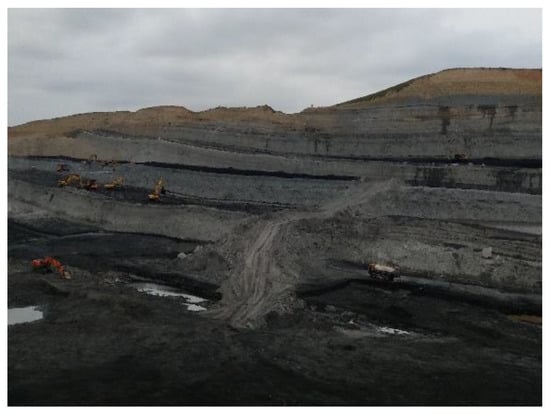
Figure 1.
Mining slope after disaster treatment.
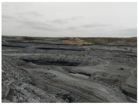
Figure 2.
Open-pit slope.
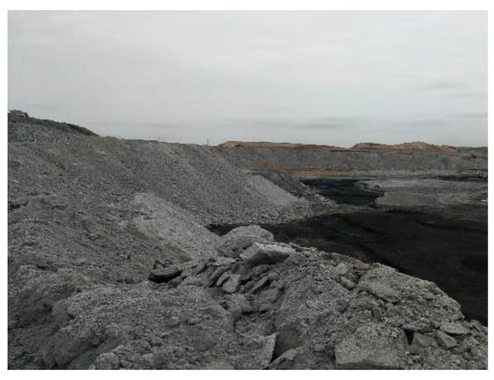
Figure 3.
Internal waste dump after disaster treatment 1.
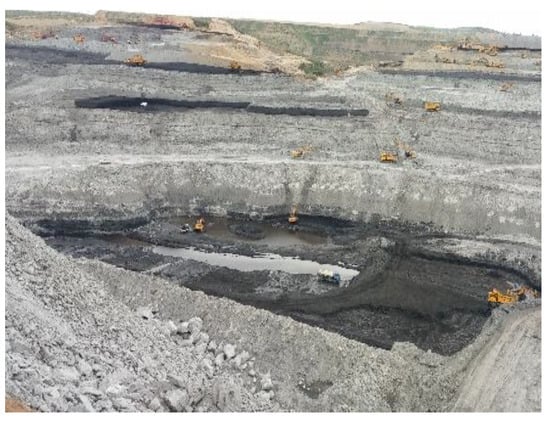
Figure 4.
Internal waste dump after disaster treatment 2.
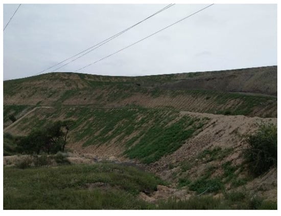
Figure 5.
External waste dump.
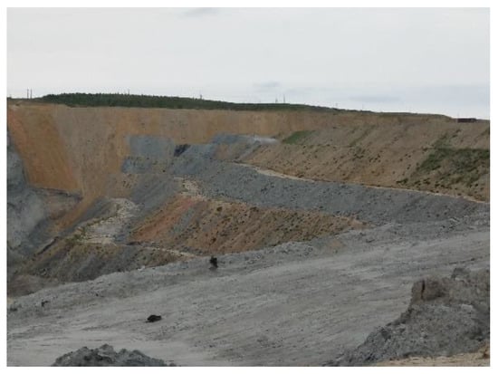
Figure 6.
Internal waste dump.
2.1. Engineering Geological Characteristics of Slope
This area is a plateau erosive hilly landform with bedrock exposed along both sides of the valley, and the ridge and valley are mainly Quaternary. Because it is located in the uplift area of the eastern edge of the Dongsheng coalfield, the upper stratum has been seriously weathered, denuded, and eroded.
2.1.1. Formation Lithology
According to the stratum exposure and borehole exposure, the main strata in the area are the Yanchang Formation of the Upper Triassic system from old to new (T3y), the middle lower Jurassic Yan’an formation (J1-2y), and the Quaternary Holocene (Q4). From old to new:
- (1)
- Yanchang Formation of Upper Triassic system (T3y)
This is the sedimentary basement of the coal measure strata. Only the southeast part of the ore field is exposed, and only the upper part is exposed by drilling. The exploration area is exposed in Ahuigou. According to the regional stratigraphic data, the thickness is > 100 m. The upper lithology is thin-layer variegated mudstone and sandy mudstone, and the lower lithology is mainly grayish-green medium and coarse-grained sandstone that is locally mixed with purple siltstone and mudstone. The sandstone is mainly composed of quartz, followed by feldspar, containing more mica fragments and dark minerals, argillaceous interstitial filling, and undeveloped bedding, and the apparent resistivity is reflected by a low amplitude relative to a formation. Large plate and trough cross bedding are developed. Only the top of the borehole is exposed, and the exposed thickness is 0~30.50 m. The thickness of the whole group is unknown.
- (2)
- A formation of middle and lower Jurassic(J1-2y)
This is the main coal bearing stratum of the ore field, which is exposed in each valley of the ore field. Its lithology is composed of a set of sandstone, siltstone, mudstone, sandy clay rock, and coal seam. The area is divided into three rock segments from bottom to top according to the lithology combination and the coal-bearing property. According to the drilling results in the ore field, only the first rock segment (J1-2y1) and the second rock segment (J1-2y2) are exposed. The exposed drilling thickness is 31.82~128.00m, with an average thickness of 84.78m.
- (1)
- The first rock section (J1-2y1): From the bottom boundary of the formation to the top boundary of coal formation 5, including three coal formations, 5, 6, and 7, the grain size of the rock in this section gradually becomes finer from bottom to top. The bottom of the lithology is mainly gray-white medium coarse-grained quartz sandstone. Local sections contain gravel. The sandstone is well-sorted and has a high quartz content. It is a regional correlation marker layer. The lithology of the middle and upper parts is interbedded with grayish-white sandstone, dark gray siltstone, and sandy mudstone containing a large number of fragment plant fossils. The surface of the area is only exposed in each valley, the control stratum thickness is about 85m, and it is in pseudointegrated contact with the underlying stratum.
- (2)
- The second rock section (J1-2y2): The area is from the coarse sandstone of the roof of the No. 5 coal formation to the bottom boundary of the sandstone of the roof of the No. 3 coal formation. The exposure in the ore field is incomplete, and only four coal groups remain. Its lithology is mainly sandy mudstone, siltstone, and mudstone intercalated with coarse-, medium-, and fine-grained sandstone, and the lower part is yellow thick-layered coarse sandstone. The rock is mainly composed of quartz, feldspar, and argillaceous cementation and is generally loose. Some sections are calcareous cementation, and the rock is spherical after weathering. The average thickness of the stratum is about 78m, with a small amount of exposure in the east of the ore field, which is in integrated contact with the underlying stratum.
- (3)
- Quaternary system (Q4): This is mainly exposed in the valley of the ore field, and the lithology is composed of an alluvial proluvial gravel layer, eluvial deluvial gravel, and secondary loess. The stratum thickness is 0~21.45m, with an average thickness of 8.49 m, and there is angular unconformity between all old strata.
2.1.2. Geological Structure
The structural form of the coal-bearing strata in the ore field is consistent with the overall structural form of the Dongsheng coalfield. It is a monoclinic structure that is inclined to the southwest, and the stratigraphic dip angle is 1~3°, with wide and gentle undulations. No obvious faults or magmatic rock intrusions are found in the ore field. The structural complexity belongs to the simple type.
2.1.3. Rock Mass Structure Type
The Quaternary System in this area is loose soil, and the coal measure stratum is a medium soft rock mass with a layered structure.
2.1.4. Engineering Geological Factors
- (1)
- Engineering geological characteristics
The ore field is located in Dongsheng Coalfield in the northeast of the Ordos Plateau. The overall terrain is high in the northwest and low in the southeast. The general elevation is 1480~1330 m. It belongs to a plateau erosive hilly landform with strong terrain cutting, exposed bedrock, and sparse vegetation. It is a semidesert area with an impermanent surface water body. No adverse engineering geological phenomena, such as debris flow and sliding wave, are found in the natural state.
- (2)
- Engineering geological characteristics of coal seam and roof and floor rock
The lithology of the coal seam roof and floor rocks in the ore field is mainly dark gray sandy mudstone and gray-white fine-grained sandstone, followed by siltstone, mudstone, and coarse-grained sandstone. According to the physical and mechanical test results of 50 groups of 129 rocks collected from five boreholes (ZK12, ZK 11, ZK 22, ZK 79, and ZK 10) constructed in the exploration report, the water content of the rocks is 4.35~15.96%, the average value of compressive strength is 3.89 MPa (the water absorption state is 0.1~3.7MPa, the natural state is 0.11~55.9 MPa), the Proctor coefficient is 0.01~2.95, the softening coefficient is 0.08~0.91, and the tensile strength is 0.21~2.89 MPa, the measured values of shear strength.
According to Table 1 and other test results, the compressive strength values of the coal seam roof and floor rocks are very low, all below 30 MPa. Sandy mudstone softens or even collapses after encountering water. Therefore, the coal seam roof and floor rocks are soft rocks.

Table 1.
List of measured values of rock shear strength.
According to the engineering geological logging results of five boreholes (ZK12, ZK11, ZK22, ZK79, and ZK10) constructed in the past, the rock joints and fissures are not very developed in the natural state, the rock core is relatively complete, the rock quality index (RQD) value is 18~89%, with an average of 66%, and the rock mass quality index (M) value is 0.0096~0.076, with an average of 0.043. Therefore, the rock quality grade in the natural state is grade III, that is, the rock quality is medium, and the rock mass is medium and complete. The rock mass quality grade is grade IV, and the rock mass quality is poor. The rocks are easily weathered after being exposed to the surface. In particular, the sandy mudstone is weathered and fragile, and the compressive strength is also significantly reduced after encountering water. Some will collapse and be destroyed in water, and the rock quality and rock mass integrity are poor.
- (3)
- Type of engineering geological exploration
The rocks are mainly clastic sedimentary rocks with layered structures and anisotropic rock mass. The strength of the coal seam roof and floor rocks is low. They are all soft rocks, and the stability of the rock mass is poor. Therefore, the engineering geological conditions are determined as three types and two types, that is, the engineering geological conditions are dominated by layered rocks of the medium type.
2.2. Determination of Physical and Mechanical Indexes of Rock and Soil Mass
According to the cohesion index of each rock stratum, an empirical reduction was adopted, combined with the engineering geological conditions of the Nayuan open-pit coal mine. The physical and mechanical indexes of the rock mass were determined, as shown in Table 2.
Table 2.
Physical and mechanical indexes of rock and soil mass.
3. Slope Stability Analysis
With the development of the computer, the slope stability can be compiled. The most dangerous sliding surface and the minimum safety factor are calculated through various optimization methods. For general rock slopes, because there are a large number of discontinuous structural planes with different occurrences and characteristics in the actual rock mass, the stability of the slope can be analyzed for a group of structural planes, controlling the slope stability according to the rigid body limit equilibrium theory, and the influence of various adverse factors can be considered.
Because the traditional rigid body limit equilibrium theory does not consider the stress–strain relationship in rock and soil mass, it is unable to analyze the occurrence and development process of slope failure and the influence of slope deformation on slope stability. Therefore, when the slope failure mechanism is complex or the stress deformation needs to be considered in slope analysis, it should be analyzed in combination with numerical simulation.
Therefore, this article adopts the combination of limit equilibrium and numerical simulation to analyze and evaluate the slope stability of the stope and waste dump of the Nayuan open-pit coal mine.
3.1. Limit Equilibrium
The limit equilibrium analysis method was the earliest method and is the most widely used analysis method in the engineering field. This method is essentially a slice method, that is, the slope body is divided into several blocks based on experience. After making appropriate assumptions about the action force on the sides of the blocks, a static balance analysis is carried out on each block, and the slope safety factor is calculated through an algebra sum [10,11].
3.1.1. Overview of Limit Equilibrium Theory
- (1)
- Definition of safety and stability factor
The slope safety factor, , refers to reducing the shear strength index of rock and soil masses to and . The rock and soil masses are in limit equilibrium along the sliding surface, as follows:
where is ; is ; is the stability coefficient; is the cohesion; and is the internal friction angle.
- (2)
- Molar Coulomb strength criterion
If a section of rock and soil mass slides along a sliding surface and the section reaches a limit equilibrium everywhere on the sliding surface, it is and that follow the Mohr–Coulomb strength criterion, which can be calculated by setting the normal force and tangential force at the bottom of the strip as and , then:
where is the dip angle of the block bottom, and the value is and is the pore water pressure, which is usually defined as the pore water pressure coefficient .
- (3)
- Force balance conditions
For the divided blocks, each block and the whole rock and soil mass need to be balanced by the force and the moment.
3.1.2. Selection of Methods
The limit equilibrium method is a common method for slope stability analysis at present. It has the characteristics of a simple calculation model, the accurate quantification of calculation parameters, and direct and practical calculation results. In the process of forming the theoretical system of the limit equilibrium method, there have been a series of simplified calculation methods, such as the Swedish method, the Bishop method, and the army engineer group method. Different calculation methods have different mechanical mechanisms, and with the emergence and development of computer, there are some methods with more strict solving steps, such as the Morgenstern–Price method, the Spencer method, and so on.
Considering that the potential modes of stope and waste dump landslides are circular sliding surface sliding and cutting bedding sliding, this study only considers the Bishop method and the Morgenstern–Price method, and the software was selected based on the principles of the two algorithms to check the slope stability. The principles of the Bishop method and the Morgenstern–Price method are described in reference [17,18], respectively.
3.2. Numerical Simulation
The slope numerical simulation of the project adopts the finite element analysis software, which is a professional software for stress and deformation analysis in geotechnical structures. It can solve linear elastic deformation problems and highly complex nonlinear elastic–plastic problems, use the total stress method and the effective stress analysis method, and perform working condition analyses, such as surcharge and excavation for soft soil consolidation analysis, and consolidation analysis, including drainage measures.
The finite element method considers the characteristics of a discontinuous medium of slope rock mass, avoids the shortcomings of the limit equilibrium method, which regards the slope as a rigid body and simplifies the boundary conditions too much, and can be close to the actual analysis of the slope stress field and the deformation field.
The finite element method can be used to solve elastic, elastoplastic, viscoelastic plastic, viscoplasticity, and other problems. The continuous system is divided into finite partitions or elements, an approximate solution is proposed for each element, and then all elements are combined into a system similar to the original system according to the standard method. The node equilibrium equations are established based on the integral principle equivalent to the differential equation and solved by the virtual work principle and the minimum potential energy principle.
- (1)
- Mathematics mechanics principle of finite element analysis
The mathematical mechanical principle and analysis steps of solving slope deformation and instability by combining the finite element method with the specific mechanical model are as follows:
① The discrete finite element calculation model is established.
With a certain form of element type (triangle or quadrilateral), the calculation model is divided into finite elements of appropriate sizes, it is assumed that the connection between each element is realized through nodes, and the load and displacement boundary conditions are determined at the same time.
② Element displacement mode analysis, element strain, and stress
Generally, the displacement mode is a polynomial of coordinates, which is written in the form of a matrix:
where is a shape function matrix and is the element node displacement matrix.
The element strain can be obtained by calculating the partial derivative of the above formula according to the following geometric equation:
where is the strain matrix.
According to the physical equation and equation (4.15), the element node displacement, , can be obtained according to the expressed element stress calculation formula:
③ Element stiffness analysis
According to the principle of virtual work, the relationship between an element node and node displacement is:
where is the element node force. is the element stiffness matrix, which can be determined by the following formula:
where is the elastic matrix.
④ Form load array
The volume force and the surface force of each element are transferred to the node of each element according to the principle of static equivalence, and the calculation formula is as follows:
where and are the equivalent node loads of the volume force and surface force acting on the element, respectively. Assuming that there are K elements around a node I, the external load, , on node I is:
where is the concentrated force acting on node I and the load array {R} is:
⑤ Form the overall balance equation
The relationship between the node force and the node displacement of each element is superimposed to form a node displacement array, , which is used in linear algebraic equations with basic unknowns:
where is the overall stiffness matrix.
⑥ Failure criterion
The Drucker–Prager criterion, which is more consistent with rock materials, is usually adopted as the failure criterion:
where and are the first and second invariants of the stress tensor and stress bias, respectively. , is the shear strength parameter of rock.
Stress transfer is carried out for the failure unit, and the transfer stress of the failure unit is:
where is the elastic–plastic matrix and the stress of the adjusted element is —.
⑦ Solution of the global equilibrium equation
To solve Equation (11), the incremental initial stress method is usually used to obtain the node displacement vector, {U}. The strain and stress of each element are calculated according to Equations (4) and (5) of the corresponding node, and the principal stress of each element is then calculated according to the stress state theory of material mechanics and the maximum principal stress , including the angle with the X axis.
3.3. Determination of Stability Reserve Coefficient
The stability reserve coefficient of the project is mainly determined according to Table 3. According to the relevant provisions of the code for Design of Open-pit Mines in Coal Industry (GB50197-2015), based on our understanding of the geological conditions of the Nayuan open-pit coal mine and our mastery of the collected data, combined with the slope retention time, the stability reserve coefficient of the project was determined as follows: the reserve value of the safety factor of the stope slope is 1.1, and that of waste dump slope is 1.2.
Table 3.
Slope stability coefficient K.
3.4. Selection of Checking Section
According to the map measured on site in August 2018 provided by the Nayuan open-pit coal mine and in combination with the actual situation of an on-site survey of the stope and waste dump, the checking section was selected. See Figure 7 for the location of each checking section.
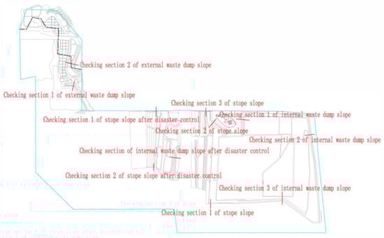
Figure 7.
The location of each checking section.
3.5. Checking Calculation of Stope Slope Stability after Disaster Control
The south side and north side of the stope slope after disaster control were selected as the two checking sections.
- (1)
- Checking section 1 of the stope slope after disaster control
The model was established according to the slope profile. The current slope is located on the north side of the stope, with a slope height of 30 m and a slope angle of 38°. The specific analysis is shown in Figure 8, Figure 9, Figure 10 and Figure 11. The movement trend of the displacement can be seen in the vector diagram. In the strain cloud diagram, it can be seen that the bottom of each step of the stope slope produces a large deformation and has a certain tensile stress on the trailing edge. The overall slope stability is good, overall sliding is unlikely, and local collapse shall be prevented. The most dangerous sliding surface was searched, and the calculated stability coefficients of the Bishop method and the Morgenstern–Price method were 1.343 > 1.1 and 1.328 > 1.1, respectively, which meet the requirements of the stability reserve coefficient, indicating that the slope is in a stable state.
Figure 8.
Schematic diagram of slope body model for checking section 1 of the stope slope after disaster control.
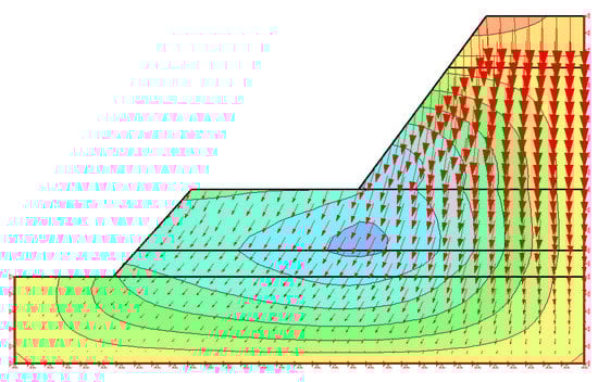
Figure 9.
Displacement motion vector diagram for checking section 1 of the stope slope after disaster control.
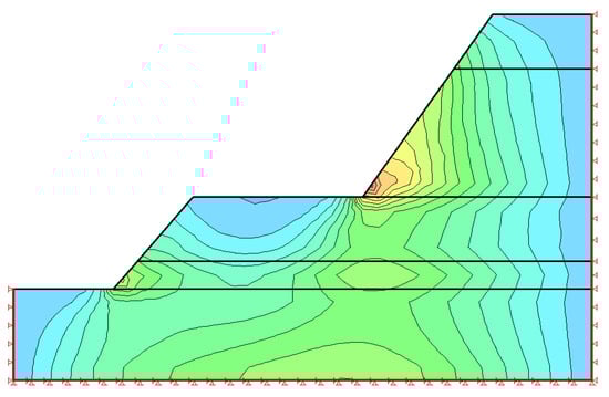
Figure 10.
Cloud diagram of shear strain for checking section 1 of the stope slope after disaster control.
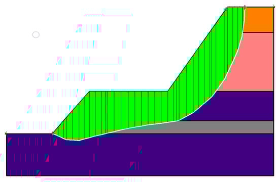
Figure 11.
Schematic diagram of limit equilibrium calculation for checking section 1 of the stope slope after disaster control.
- (2)
- Checking section 2 of the stope slope after disaster control
The model was established according to the slope profile. The current slope is located on the south side of the stope, with a slope height of 30 m and a slope angle of 34°. The specific analysis is shown in Figure 12, Figure 13, Figure 14 and Figure 15. The movement trend of the displacement can be seen in the vector diagram. In the strain cloud diagram, it can be seen that there is large deformation at the bottom of the stope slope step, and there is a certain tensile stress on the trailing edge. The overall slope stability is good, overall sliding is unlikely, and local collapse shall be prevented. The most dangerous sliding surface was searched, and the calculated stability coefficients of the Bishop method and the Morgenstern–Price method were 1.362 > 1.1 and 1.356 > 1.1, respectively, which meet the requirements of the stability reserve coefficient, indicating that the slope is in a stable state.
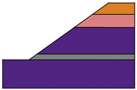
Figure 12.
Schematic diagram of slope body model for checking section 2 of the stope slope after disaster control.
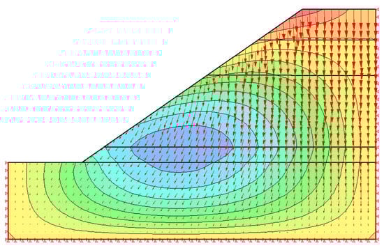
Figure 13.
Displacement motion vector diagram for checking section 2 of the stope slope after disaster control.
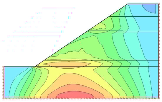
Figure 14.
Cloud diagram of shear strain for checking section 2 of the stope slope after disaster control.
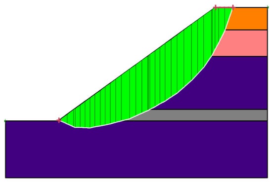
Figure 15.
Schematic diagram of limit equilibrium calculation for checking section 2 of the stope slope after disaster control.
3.6. Checking Calculation of Stope Slope Stability in Open-Pit Mine
The south side, east side, and north side of the stope were selected as three checking sections.
- (1)
- Checking section 1 of the stope slope
The model was established according to the slope profile. The current slope is located on the south side of the stope, with a slope height of 15 m and a slope angle of 37°. The specific analysis is shown in Figure 16, Figure 17, Figure 18 and Figure 19. The displacement movement trend can be seen in the vector diagram. In the strain cloud diagram, it can be seen that there is a large deformation at the bottom of the stope slope, and there is a certain tensile stress on the trailing edge. The overall slope stability is good, and the overall sliding possibility is small. Therefore, local collapse shall be prevented. The most dangerous sliding surface was searched, and the calculated stability coefficients of the Bishop method and the Morgenstern–Price method were 1.423 > 1.1 and 1.419 > 1.1, respectively, which meet the requirements of the stability reserve coefficient, indicating that the slope is in a stable state.
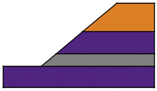
Figure 16.
Schematic diagram of slope body model for checking section 1 of the stope slope.
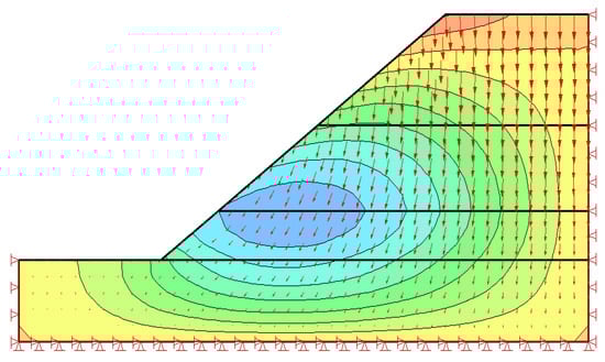
Figure 17.
Displacement motion vector diagram for checking section 1 of the stope slope.
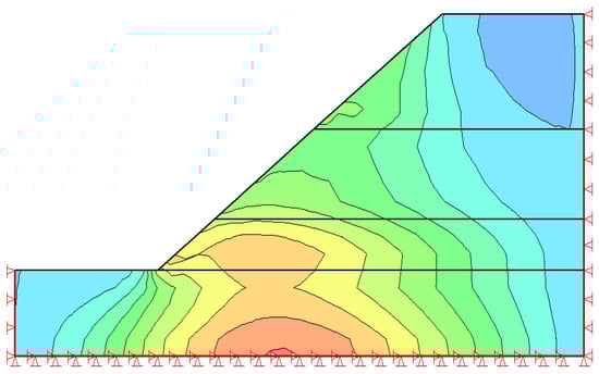
Figure 18.
Cloud diagram of shear strain for checking section 1 of the stope slope.
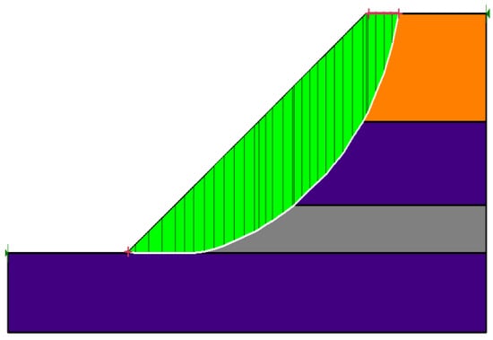
Figure 19.
Schematic diagram of limit equilibrium calculation for checking section 1 of the stope slope.
- (2)
- Checking section 2 of the stope slope
The model was established according to the slope profile. The current slope is located on the east side of the stope, with a slope height of 30 m and a slope angle of 25°. The specific analysis is shown in Figure 20, Figure 21, Figure 22 and Figure 23. The movement trend of the displacement can be seen in the vector diagram. In the stress cloud diagram, it can be seen that there is a large deformation at the bottom of the stope slope, and there is a certain tensile stress on the trailing edge. The overall slope stability is good, and the overall sliding possibility is small. Therefore, local collapse shall be prevented. The most dangerous sliding surface was searched, and the calculated stability coefficients were 1.378 > 1.1 by the Bishop method and 1.374 > 1.1 by the Morgenstern–Price method, which meet the requirements of the stability reserve coefficient, indicating that the slope is in a stable state.
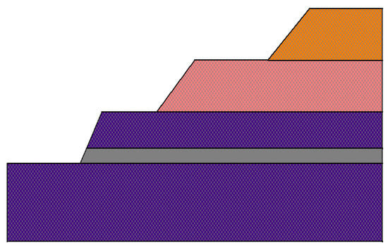
Figure 20.
Schematic diagram of slope body model for checking section 2 of the stope slope.
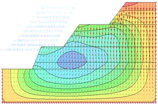
Figure 21.
Displacement motion vector diagram for checking section 2 of the stope slope.
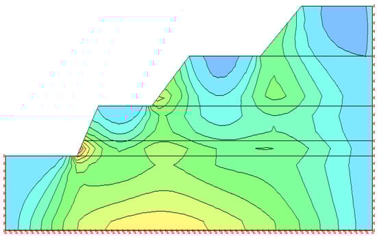
Figure 22.
Cloud diagram of shear strain for checking section 2 of the stope slope.
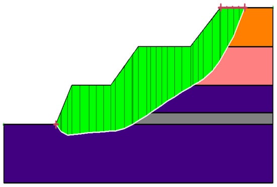
Figure 23.
Schematic diagram of limit equilibrium calculation for checking section 2 of the stope slope.
- (3)
- Checking section 3 of the stope slope
The model was established according to the slope profile. The current slope is located on the north side of the stope, with a slope height of 40 m and a slope angle of 47°. The specific analysis is shown in Figure 24, Figure 25, Figure 26 and Figure 27. The movement trend of the displacement can be seen in the vector diagram. In the stress cloud diagram, it can be seen that there is a large deformation at the bottom of the stope slope, and there is a certain tensile stress on the trailing edge. The overall slope stability is good, and the overall sliding possibility is small. Therefore, local collapse shall be prevented. The most dangerous sliding surface was searched, and the calculated stability coefficients of the Bishop method and the Morgenstern–Price method were 1.161 > 1.1 and 1.157 > 1.1, respectively, which meet the requirements of the stability reserve coefficient, indicating that the slope is in a stable state.
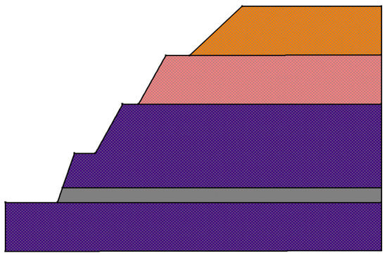
Figure 24.
Schematic diagram of slope body model for checking section 3 of the stope slope.
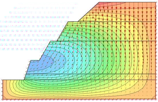
Figure 25.
Displacement motion vector diagram for checking section 3 of the stope slope.
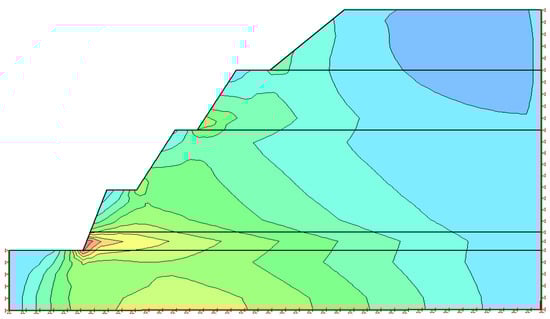
Figure 26.
Cloud diagram of shear strain for checking section 3 of the stope slope.
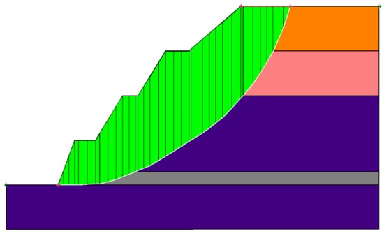
Figure 27.
Schematic diagram of limit equilibrium calculation for checking section 3 of the stope slope.
3.7. Checking Calculation of Slope Stability of Waste Dump after Disaster Control
The east side of the internal waste dump after disaster control was selected as the checking section.
The model was established according to the slope profile. The current slope is 55 m high with a slope angle of 25°. The specific analysis is shown in Figure 28, Figure 29, Figure 30 and Figure 31. The displacement movement trend can be seen in the vector diagram. In the stress cloud diagram, it can be seen that the slope at the bottom of the waste dump slope has a large deformation and has a certain tensile stress on the trailing edge. At present, the overall slope stability is good. Overall sliding is unlikely, and local collapse shall be prevented. The most dangerous sliding surface was searched, and the calculated stability coefficients were 1.263 > 1.2 by the Bishop method and 1.257 > 1.2 by the Morgenstern–Price method, which meet the requirements of the stability reserve coefficient, indicating that the slope is in a stable state.
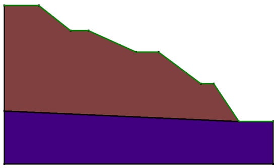
Figure 28.
Schematic diagram of slope body model for checking section of slope stability of waste dump after disaster control.
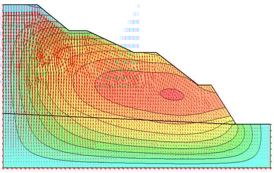
Figure 29.
Displacement motion vector diagram for checking section of slope stability of waste dump after disaster control.
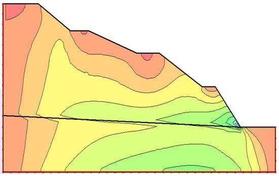
Figure 30.
Cloud diagram of shear strain for checking section of slope stability of waste dump after disaster control.
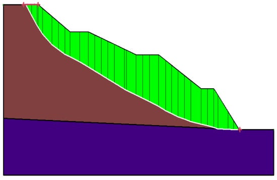
Figure 31.
Schematic diagram of limit equilibrium calculation for checking section of slope stability of waste dump after disaster control.
3.8. Checking Calculation of Slope Stability of Open-Pit Waste Dump
The southeast and east sides of the external waste dump and the west, east, and south sides of the internal waste dump were selected as five checking sections.
- (1)
- Main factors affecting the stability of the waste dump
The waste materials in the waste dump of the Nayuan open-pit coal mine are loose, and the cohesion is low. In particular, the strength of the mudstone and sandy mudstone in the waste materials in contact with water was significantly weakened, reducing the stability of waste dump. The main factors affecting the stability of the waste dump include: the basement, surface, and quaternary phreatic water, the waste material load, etc.
1) Waste dump basement: according to the coal production exploration report of the Nayuan open-pit coal mine in the Tongjiangchuan detailed survey area of Dongsheng coalfield, Inner Mongolia Autonomous Region, the lithology of the waste dump basement is mainly sandy mudstone and mudstone, with good stability, but waterproofing and drainage shall be carried out effectively.
2) Diving: due to the increase in the water content in the waste caused by atmospheric precipitation and other water, the mechanical strength indexes of the waste and the base are weakened, which increases the sliding force and reduces the antisliding force.
3) Waste load: the higher the waste height of the waste dump and the steeper the slope angle of the waste dump, the greater the pressure on the base and the easier it is to produce bottom heave.
- (2)
- Checking the calculation of the slope stability of the waste dump
1) Checking section 1 of the external waste dump slope
The model was established according to the slope profile. The current slope is 60 m high with a slope angle of 32° and is located on the southeast side of the external waste dump. The specific analysis is shown in Figure 32, Figure 33, Figure 34 and Figure 35. The movement trend of the displacement can be seen in the vector diagram. In the stress cloud diagram, it can be seen that the slope at the bottom of the waste dump slope produces a large deformation and has a certain tensile stress on the trailing edge. At present, the overall slope stability is good. Overall sliding is unlikely, and local collapse shall be prevented. The most dangerous sliding surface was searched, and the calculated stability coefficients were 1.203 > 1.2 by the Bishop method and 1.201 > 1.2 by the Morgenstern–Price method, which meet the requirements of the stability reserve coefficient, indicating that the slope is in a stable state.
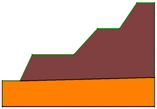
Figure 32.
Schematic diagram of slope body model for checking section 1 of the external waste dump slope.
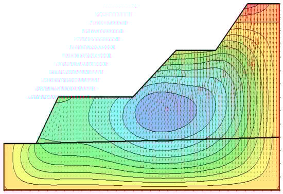
Figure 33.
Displacement motion vector diagram for checking section 1 of the external waste dump slope.
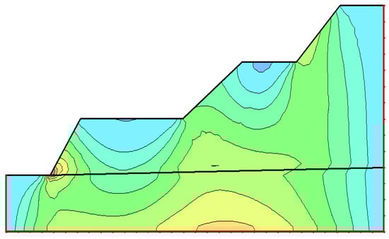
Figure 34.
Cloud diagram of shear strain for checking section 1 of the external waste dump slope.
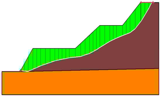
Figure 35.
Schematic diagram of limit equilibrium calculation for checking section 1 of the external waste dump slope.
2) Checking section 2 of the external waste dump slope
The model was established according to the slope profile. The current slope is 60 m high with a slope angle of 16° and is located on the east side of the external waste dump. The specific analysis is shown in Figure 36, Figure 37, Figure 38 and Figure 39. The displacement movement trend can be seen in the vector diagram. In the stress cloud diagram, it can be seen that the top of each step of the waste dump slope has a large deformation and has a certain tensile stress on the trailing edge. The overall slope stability is good. Overall sliding is unlikely, and local collapse shall be prevented. The most dangerous sliding surface was searched, and the calculated stability coefficients were 1.313 > 1.2 by the Bishop method and 1.312 > 1.2 by the Morgenstern–Price method, which meet the requirements of the stability reserve coefficient, indicating that the slope is in a stable state.
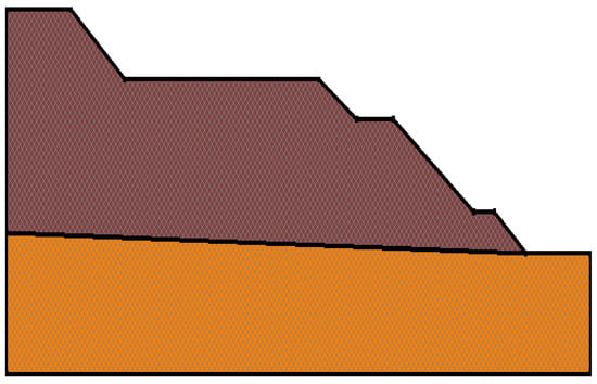
Figure 36.
Schematic diagram of slope body model for checking section 2 of the external waste dump slope.
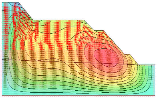
Figure 37.
Displacement motion vector diagram for checking section 2 of the external waste dump slope.
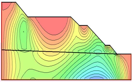
Figure 38.
Cloud diagram of shear strain for checking section 2 of the external waste dump slope.
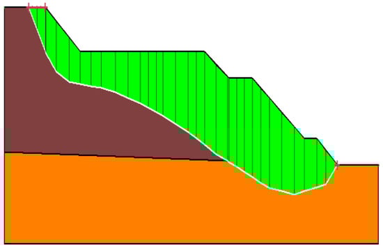
Figure 39.
Schematic diagram of limit equilibrium calculation for checking section 2 of the external waste dump slope.
- (3)
- Checking section 1 of the inner waste slope
The model was established according to the slope profile. The current slope is 50 m high with a slope angle of 30° and is located on the west side of the inner waste dump. The specific analysis is shown in Figure 40, Figure 41, Figure 42 and Figure 43. The displacement movement trend can be seen in the vector diagram. In the stress cloud diagram, it can be seen that the slope at the bottom of the waste dump has large deformation and has a certain tensile stress on the trailing edge. The overall slope stability is good. Overall sliding is unlikely, and local collapse shall be prevented. The most dangerous sliding surface was searched, and the calculated stability coefficients were 1.218 > 1.2 by the Bishop method and 1.214 > 1.2 by the Morgenstern–Price method, which meet the requirements of the stability reserve coefficient, indicating that the slope is in a stable state.
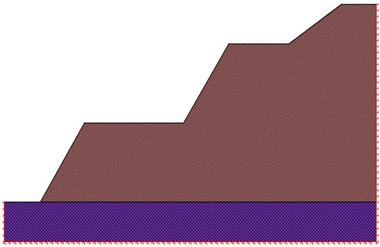
Figure 40.
Schematic diagram of slope body model for checking section 1 of the inner waste slope.
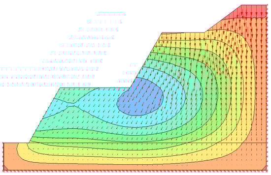
Figure 41.
Displacement motion vector diagram for checking section 1 of the inner waste slope.
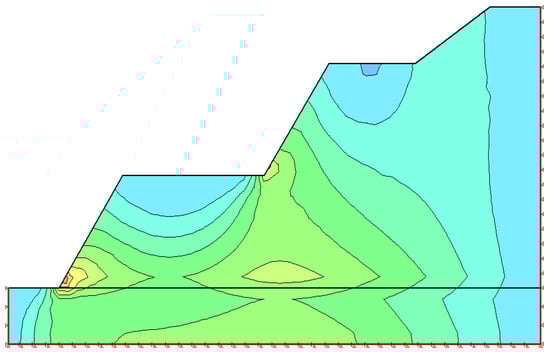
Figure 42.
Cloud diagram of shear strain for checking section 1 of the inner waste slope.
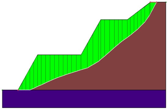
Figure 43.
Schematic diagram of limit equilibrium calculation for checking section 1 of the inner waste slope.
- (4)
- Checking section 2 of the inner waste dump slope
The model was established according to the slope profile. The current slope is 50 m high with a slope angle of 25° and is located on the east side of the inner waste dump. The specific analysis is shown in Figure 44, Figure 45, Figure 46 and Figure 47. The movement trend of the displacement can be seen in the vector diagram. In the stress cloud diagram, it can be seen that the top and bottom slopes of the waste dump slope produce large deformations and have certain tensile stresses on the trailing edges. The overall slope stability is good. Overall sliding is unlikely, and local collapse shall be prevented. The most dangerous sliding surface was searched, and the calculated stability coefficients were 1.227 > 1.2 by the Bishop method and 1.226 > 1.2 by the Morgenstern–Price method, which meet the requirements of the stability reserve coefficient, indicating that the slope is in a stable state.
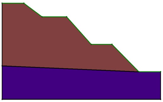
Figure 44.
Schematic diagram of slope body model for checking section 2 of the inner waste slope.
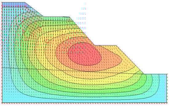
Figure 45.
Displacement motion vector diagram for checking section 2 of the inner waste slope.
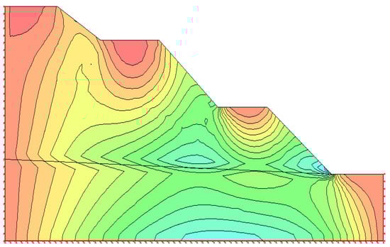
Figure 46.
Cloud diagram of shear strain for checking section 2 of the inner waste slope.
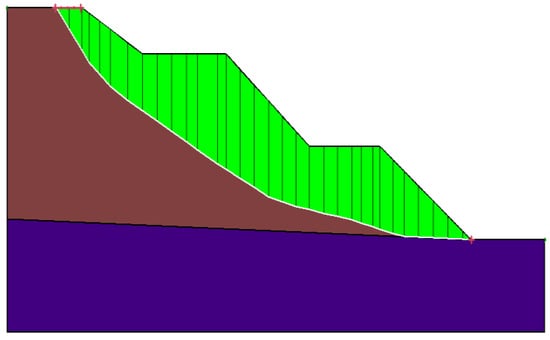
Figure 47.
Schematic diagram of limit equilibrium calculation for checking section 2 of the inner waste slope.
- (5)
- Checking section 3 of the inner waste dump slope
The model was established according to the slope profile. The current slope is 60 m high with a slope angle of 24° and is located on the south side of the inner waste dump. The specific analysis is shown in Figure 48, Figure 49, Figure 50 and Figure 51. The movement trend of the displacement can be seen in the vector diagram. In the stress cloud diagram, it can be seen that there is a large deformation at the bottom of the waste dump slope, which has a certain tensile stress on the trailing edge, and the overall slope stability is good. Overall sliding is unlikely, and local collapse shall be prevented. The most dangerous sliding surface was searched, and the calculated stability coefficients of the Bishop method and the Morgenstern–Price method were 1.231 > 1.2 and 1.229 > 1.2, respectively, which meet the requirements of the stability reserve coefficient, indicating that the slope is in a stable state.
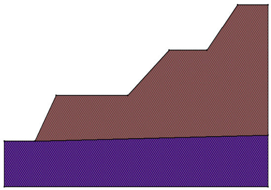
Figure 48.
Schematic diagram of slope body model for checking section 3 of the inner waste slope.
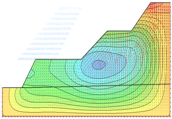
Figure 49.
Displacement motion vector diagram for checking section 3 of the inner waste slope.
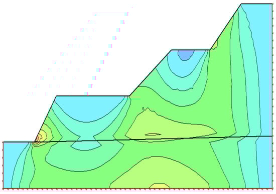
Figure 50.
Cloud diagram of shear strain for checking section 3 of the inner waste slope.
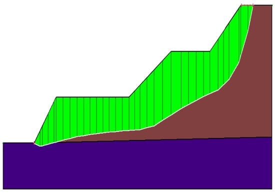
Figure 51.
Schematic diagram of limit equilibrium calculation for checking section 3 of the inner waste slope.
3.9. Evaluation Results
Through the field survey of the Nayuan open-pit coal mine, aiming at the stope and waste dump slopes of its disaster control pit and open-pit, the slope stability was comprehensively checked and analyzed using the limit equilibrium method (Bishop method and Morgenstern–Price method) and numerical simulation. The main results are shown in Table 4.
Table 4.
Table of checking calculation and simulation results of slope safety factor of each section.
It can be seen in Table 4 that the geological conditions of the base of the waste dump of the mine are good, and the stope slopes and waste dump are stable, meeting the requirements of 6.0.7 in the code for Design of Open-pit Mines in Coal Industry (GB 50197-2015).
4. Conclusions and Recommendations
4.1. Conclusions
By means of an engineering geology and hydrogeological investigation of the waste dump area of the Nayuan open-pit coal mine and numerical simulation research, the stability of the stope and the waste dump slope of the Nayuan open-pit coal mine was analyzed and studied in detail, and slope prevention, automatic monitoring, and other measures are put forward to achieve the goal of protecting the stope and waste dump slope and the surrounding environment. The main research results are summarized as follows:
- (1)
- The geotechnical physical and mechanical indexes of the stope and the waste dump were collected and analyzed, and the geotechnical mechanical indexes in this report were determined, which basically meet the requirements of slope stability analysis.
- (2)
- The limit equilibrium method and finite element method were used to analyze and evaluate the current slope stability of the Nayuan open-pit coal mine. It was concluded that the foundation of the waste dump is basically stable, and the potential landslide modes of the slope are arc-shaped sliding surface and arc-shaped linear sliding surface. The numerical simulation and checking results show that the current stope and waste dump slope are stable.
- (3)
- Checking section 1 of the stope slope after disaster control is 30 m high, the slope angle is 38°, and the stability coefficients calculated by the Bishop method and the Morgenstern–Price method are 1.343 > 1.1 and 1.328 > 1.1, respectively. Checking section 2 of the stope slope after disaster control is 30 m high, the slope angle is 34°, and the stability coefficients calculated by the Bishop method and the Morgenstern–Price method are 1.362 > 1.1 and 1.356 > 1.1, respectively. Checking section 1 of the stope slope is 15 m high, the slope angle is 37°, and the stability coefficient calculated by the Bishop method and the Morgenstern–Price method are 1.423 > 1.1 and 1.419 > 1.1, respectively. Checking section 2 of the stope slope is 30 m high, and the slope angle is 25°. The stability coefficients calculated by the Bishop method and the Morgenstern–Price method are 1.378 > 1.1 and 1.374 > 1.1, respectively. Checking section 3 of the stope slope is 40 m high, and the slope angle is 47°. The stability coefficients calculated by the Bishop method and the Morgenstern–Price method are 1.161 > 1.1 and 1.157 > 1.1, respectively. The slope stability checking section of the waste dump after disaster control is 55 m high, and the slope angle is 25°. The stability coefficient calculated by the Bishop method is 1.263 > 1.2, and that calculated by the Morgenstern–Price method is 1.257 > 1.2. Checking calculation profile 1 of the waste dump slope is 60 m high, the slope angle is 32°, and the stability coefficients calculated by the Bishop method and the Morgenstern–Price method are 1.203 > 1.2 and 1.201 > 1.2, respectively. Checking calculation profile 2 of the waste dump slope is 60 m high, the slope angle is 16°, and the stability coefficients calculated by the Bishop method and the Morgenstern–Price method are 1.313 > 1.2 and 1.312 > 1.2, respectively. Checking section 1 of the internal waste dump slope is 50 m high, and the slope angle is 30°. The stability coefficient calculated by the Bishop method is 1.218 > 1.2, and that calculated by the Morgenstern–Price method is 1.214 > 1.2. Slope checking section 2 of the inner waste dump is 50 m high, and the slope angle is 25°. The stability coefficient calculated by the Bishop method is 1.227 > 1.2, and that calculated by the Morgenstern–Price method is 1.226 > 1.2. Slope checking section 3 of the inner waste dump is 60 m high, and the slope angle is 24°. The stability coefficient calculated by the Bishop method is 1.231 > 1.2, and that calculated by the Morgenstern–Price method is 1.229 > 1.2.
4.2. Recommendations
This study was only conducted under the existing engineering geological and hydrogeological survey conditions. It is suggested that the following work be carried out:
- (1)
- Attach great importance to the slope management of the stope and the waste dump, and establish and improve the slope safety management organization system.
- (2)
- Strengthen slope deformation monitoring and rapidly assess the dynamic situation and the law of slope deformation, conduct real-time monitoring of the stope and waste dump slopes, and assign special personnel for supervision. Once signs of a landslide are found, evacuate personnel and equipment immediately and carry out a special investigation, evaluation, and treatment engineering design for any local and small-scale slope collapses and slides.
- (3)
- This paper checked and analyzed the slope according to the actual situation of the coal mine, which is only applicable to the current stage. It is suggested that the coal mine should carry out mining and stripping operations in strict accordance with the design and specification requirements in the future production process, strengthen slope monitoring, take prevention measures immediately when there are signs of a landslide on the slope, and organize the evacuation of personnel and equipment as soon as possible to ensure the safety of personnel and equipment.
Author Contributions
Conceptualization, J.C.; methodology, J.C.; software, X.D.; validation, J.C. and X.D.; formal analysis, J.C.; investigation, X.D.; resources, X.D.; data curation, X.D.; writing—original draft preparation, J.C.; writing—review and editing, J.C.; visualization, J.C.; supervision, X.D.; project administration, X.D.; funding acquisition, X.D. All authors have read and agreed to the published version of the manuscript.
Funding
This research was funded by the Science and Technology Innovation Project of China Energy Investment Group Co., Ltd., grant number GJNY-20-231.
Data Availability Statement
The data used to support the findings of this study are available within the article.
Acknowledgments
Thanks to Yan Du of the Beijing University of Science and Technology for his support in the numerical calculations in this paper.
Conflicts of Interest
The authors declare no conflict of interest.
References
- Zhu, X. Application of Gravity Increase Method in Slope Stability Analysis; Xi’an University of Science and Technology: Xi’an, China, 2010. [Google Scholar]
- Kong, D. Analysis Theory and Practice of Slope Stability; Hefei University of Technol: Hefei, China, 2009. [Google Scholar]
- Cundall, P.A. Formulation of a three-dimensional distinct element model—Part I: A scheme to detect and represent contacts in a system composed of many polyhedral blocks. Int. J. Rock Mech. Min. Sci. Geomech. Abstr. 1988, 25, 107–116. [Google Scholar] [CrossRef]
- Zienkiewicz, O.C.; Humpheson, C.; Lewis, R.W. Associated and non—Associated viseo-plasticity and plasticity in soil mechanics. Geotechnique 1975, 25, 671–689. [Google Scholar] [CrossRef]
- Ghaboussi, J.R.; Barboosa, R. Three-dimensional and discrete element methods for granular material. Int. J. Numer. Anal. Methods Geomech. 1990, 14, 451–472. [Google Scholar] [CrossRef]
- Shi, G.H. Numerical Manifold Method and Discontinuous Deformation Analysis; Pei, J.M., Translator; Tsinghua University Press: Beijing, China, 1997. [Google Scholar]
- Zhuo, J.S.; Zhang, Q. Interface Element Method for Mechanical Problems of Discontinuous Media; Pei, J.M., Translator; Science Press: Beijing, China, 2000. [Google Scholar]
- Wu, S.C.; Jin, A.B.; Liu, Y. Slope Engineering; Metallurgical Industry Press: Beijing, China, 2020. [Google Scholar]
- Jin, F.C. Research status and Prospect of slope stability methods. West-China Explor. Eng. 2007, 4, 5–6. [Google Scholar]
- Wang, Y.P. Summary of slope stability analysis methods. J. Xihua Univ. 2012, 31, 101–102. [Google Scholar]
- Xiang, J. Study on Stability Analysis and Prevention of Cutting Slope of Tongping Expressway; Central South University: Changsha, China, 2011. [Google Scholar]
- Zhu, C.B. Analysis and Evaluation of Slope Stability—Taking the Slope of Yuanjiang-Mohei Expressway as an Example; Kunming University of Technology: Kunming, China, 2005. [Google Scholar]
- Wang, J.C. Stochastic Analysis Principle of Slope Engineering; Coal Industry Press: Beijing, China, 1996. [Google Scholar]
- Chen, X.M.; Luo, G.H. Grey system analysis and evaluation of slope stability based on experience. J. Geotech. Eng. 1999, 21, 638–641. [Google Scholar]
- Wang, Y.X. Application of fuzzy mathematics in slope stability analysis. J. Geotech. Eng. 2010, 31, 30. [Google Scholar]
- Xiong, H.F. Study on Slope Stability Evaluation Based on Artificial Neural Network Technology; Wuhan University of Technology: Wuhan, China, 2003. [Google Scholar]
- Bishop, A.W. The use of the slip circle in the stability analysis of slopes. Geothenique 1955, 5, 7–17. [Google Scholar] [CrossRef]
- Morgenstern, N.R.; Price, V.E. The analysis of the stability of general slip surface. Geotechnique 1965, 15, 79–93. [Google Scholar] [CrossRef]
- Cheng, J. Residential land leasing and price under public land ownership. J. Urban Plan. Dev. 2021, 147, 05021009. [Google Scholar] [CrossRef]
- Cheng, J. Analysis of commercial land leasing of the district governments of Beijing in China. Land Use Policy 2021, 100, 104881. [Google Scholar] [CrossRef]
- Cheng, J. Analyzing the factors influencing the choice of the government on leasing different types of land uses: Evidence from Shanghai of China. Land Use Policy 2020, 90, 104303. [Google Scholar] [CrossRef]
- Cheng, J. Data analysis of the factors influencing the industrial land leasing in Shanghai based on mathematical models. Math. Probl. Eng. 2020, 2020, 9346863. [Google Scholar] [CrossRef]
- Cheng, J. Mathematical models and data analysis of residential land leasing behavior of district governments of Beijing in China. Mathematics 2021, 9, 2314. [Google Scholar] [CrossRef]
- Zheng, G.D.; Cheng, Y.M. The improved element-free Galerkin method for diffusional drug release problems. Int. J. Appl. Mech. 2020, 12, 2050096. [Google Scholar] [CrossRef]
- Wu, Q.; Peng, P.P.; Cheng, Y.M. The interpolating element-free Galerkin method for elastic large deformation problems. Sci. China Technol. Sci. 2021, 64, 364–374. [Google Scholar] [CrossRef]
- Cheng, H.; Peng, M.J.; Cheng, Y.M. The hybrid complex variable element-free Galerkin method for 3D elasticity problems. Eng. Struct. 2020, 219, 110835. [Google Scholar] [CrossRef]
- Li, J.; Wu, J. Study on elastoplastic damage constitutive model of concrete I:Basic formula. J. Civ. Eng. 2005, 38, 14–20. [Google Scholar]
- Wu, J. The elastoplastic Damage Constitutive Model of Concrete Based on the Damage Energy Release Rate and the Application in Structural Nonlinear Analysis. Ph.D. Thesis, Tongji University, Shanghai, China, 2004. [Google Scholar]
- Ma, W.B.; Chai, J.F.; Li, Z.F.; Han, Z.L.; Ma, C.F.; Li, Y.J.; Zhu, Z.Y.; Liu, Z.Y.; Niu, Y.B.; Ma, Z.G.; et al. Research on vibration Law of railway tunnel substructure under different axle loads and health conditions. Shock Vib. 2021, 2021, 9954098. [Google Scholar] [CrossRef]
- Han, Z.L.; Ma, W.B.; Chai, J.F.; Zhu, Z.Y.; Lin, C.N.; An, Z.L.; Ma, C.F.; Xu, X.L.; Xu, T.Y. A Treatment Technology for Optimizing the Stress State of Railway Tunnel Bottom Structure. Shock Vib. 2021, 2021, 9191232. [Google Scholar] [CrossRef]
- Ma, W.B.; Chai, J.F.; Han, Z.L.; Ma, Z.G.; Guo, X.X.; Zou, W.H.; An, Z.L.; Li, T.F.; Niu, Y.B. Research on Design Parameters and Fatigue Life of Tunnel Bottom Structure of Single-Track Ballasted Heavy-Haul Railway Tunnel with 40-Ton Axle Load. Math. Probl. Eng. 2020, 2020, 3181480. [Google Scholar] [CrossRef]
- Chai, J.F. Research on Multijoint Rock Failure Mechanism Based on Moment Tensor Theory. Math. Probl. Eng. 2020, 2020, 6816934. [Google Scholar] [CrossRef]
Publisher’s Note: MDPI stays neutral with regard to jurisdictional claims in published maps and institutional affiliations. |
© 2022 by the authors. Licensee MDPI, Basel, Switzerland. This article is an open access article distributed under the terms and conditions of the Creative Commons Attribution (CC BY) license (https://creativecommons.org/licenses/by/4.0/).