Article

Efficiency and Core Loss Map Estimation with Machine Learning Based Multivariate Polynomial Regression Model

1
Department of Electronics and Automation, Turhal Vocational School, Tokat Gaziosmanpaşa University, Tokat 60150, Turkey
2
Department of Electric-Electronic Engineering, Faculty of Engineering and Architecture, Tokat Gaziosmanpaşa University, Tokat 60150, Turkey
*
Author to whom correspondence should be addressed.
Mathematics 2022, 10(19), 3691; https://doi.org/10.3390/math10193691
Submission received: 30 August 2022 / Revised: 4 October 2022 / Accepted: 7 October 2022 / Published: 9 October 2022

Abstract

:
Efficiency mapping has an important place in examining the maximum efficiency distribution as well as the energy consumption of designed electric motors at maximum torque and speed. Performing analysis at all operating points with FEM analysis in the motor design process requires high processing costs and time. In this article, a machine learning-based multivariate polynomial regression estimation model was developed to overcome these costly processes from FEM analysis. With the proposed method, the operating points of the motors in different conditions during the design process can be predicted in advance with high accuracy. In the study, two different models are developed for efficiency map and core loss estimation of interior permanent magnet synchronous motor design. The developed models use few parameters and predict with high accuracy. Estimation models shorten the design process and offer a less complex model. Obtained results are validated by comparison with FEM analysis.

Graphical Abstract

1. Introduction

Systems using electric motors have a large place in global energy consumption, while their CO2 emissions grow at significant rates [1]. Well-sized and optimized motor systems with all their components play a key role in reducing this negative effect. The most emphasized issue in studies of electric vehicles is how to extend the vehicle range as much as possible according to the current battery capacity and weight of the vehicle. This can only be achieved by the operation of electric vehicle components within maximum efficiency regions. The most important and energy-consuming components of electric vehicles are electric motors. While these motors provide the power/torque values required for acceleration and hill climbing, they also need to be as efficient as possible. For this reason, the efficiency map for the motors used in these vehicles or predicting these values as in the proposed method plays a key role in both more efficient and widespread use of electric vehicles. Especially with the development of power electronics components, induction motors are frequently used in variable speed applications. These motors are preferred because of their simple structure, low need for maintenance, and high efficiency at nominal operating points [2]. However, rotor copper losses and accordingly low thermal load ability are the biggest disadvantages of these motors. Especially in electric vehicle applications, motors containing magnets are often preferred [3,4,5,6]. However, interior permanent magnet synchronous motors (IPMSMs), some of the most often used motors in electric vehicles, are very popular due to their high torque density, high efficiency, wide speed range, and reluctance torque in addition to magnet torque [7,8]. Motors used in electric vehicles are operated in a wide speed-torque range. Hence, in motor selection, vehicle characteristics such as vehicle weight and aerodynamics, as well as how the vehicle is used, play a key role in determining the required speed, torque, and power values of the vehicle. In addition, whether the vehicle is a hybrid or pure electric vehicle; what is the required maximum speed, torque, and power values; what is battery capacity and voltage; whether the motor has a direct drive or a gearbox; and the cost, which is the most important factor, are other important factors affecting the selection of the motor. Efficiency class standards [9] of motors used in industry mostly test motors in constant speed applications such as pumps, fans, and compressors, and IE1, IE2, IE3, and IE4 class standards are determined for these motors [10]. There is no current regulation that determines the efficiency class of motors used in electric vehicles and motors manufactured for industrial purposes. Motor efficiency mapping is an important issue in electric motor design. This graph (efficiency map), which is given as a function of the maximum torque produced by the motor depending on the motor speed and efficiency, is crucial in determining the area where the electric motor is most efficient in different driving combinations, especially when presented with the drive cycle. In addition, parameters such as motor total losses, d q axis flux and current values, and copper losses are also determined within voltage and current limits [6]. However, while doing this, the current, current angle, voltage, and torque values applied to the motor windings at each operating point, as well as the rotor speed and position, can be recorded in appropriate resolution. The motor efficiency map determination is carried out experimentally, through the analytical model or by analyzing the Finite Element Model (FEM) of the motor [11]. In the experimental method, in addition to the motor shaft power, the voltages applied to the motor windings and the currents drawn can also be recorded. This is possible once the drive motor is manufactured and ready for testing. However, prototyping and testing process steps must be carried out repeatedly for improvements after experimental results. This process is both costly and time consuming. In the FEM method, time-dependent transient analysis is usually performed on the 2D or 3D model created depending on the physical dimensions, material properties, and winding structure of the motor. In this method, these analyses can be repeated for different current, current angle, and speed values. However, analysis at different operating points, especially with the FEM method, is very time-consuming in terms of both time and processor load. This situation becomes inescapable in cases such as the model being 3D, whether it contains a skew or not.
In this study, a new method is presented using machine learning based multivariate polynomial regression to eliminate these deficiencies and accelerate the process. To verify and test the developed method, the data of the IPMSM modeled with the FEM method were used, and the results obtained were presented comparatively for different velocity, current and current angle values. The estimation of motor efficiency parameters using learning algorithms has attracted considerable attention by researchers in the motor design process [12]. In recent studies, Deep learning (DL) and Neural Network (NN) methods have been used for efficiency map estimation [13,14]. The main contribution emphasized in these studies is the reduction of the design process of the modeled motor compared to the FEM method. In the proposed method, in addition to the reduction of the design process, a multivariate polynomial regression model is used, and a model that can make predictions with high accuracy using fewer model parameters has been developed.

2. Materials and Methods

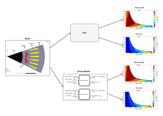
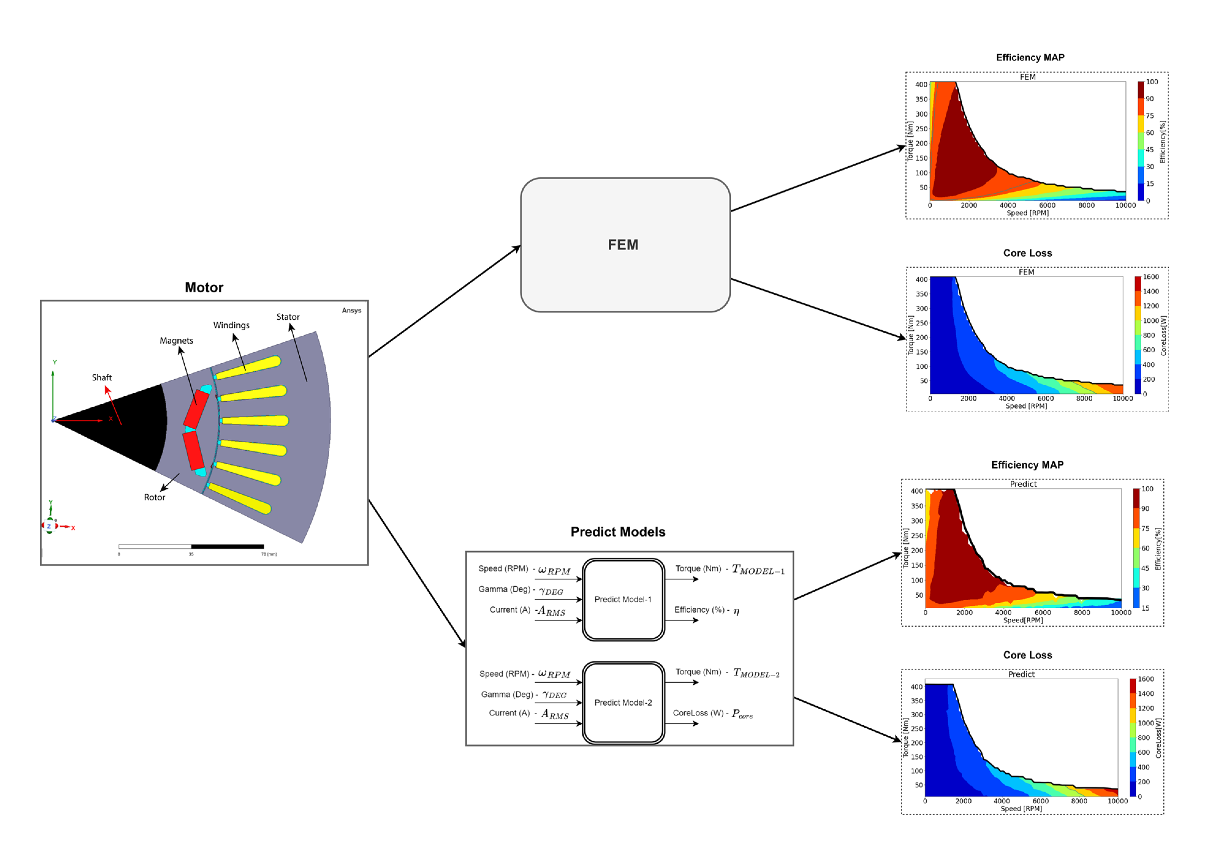
2.1. IPMSM FEM Model and Efficiency Map Calculation

The IPMSM used in the modeling is shown in Figure 1. The analyzed motor has a power of 50 kW and a torque of 400 Nm. Detailed information about the motor is presented in Table 1 [15,16]. In the designed motor, the oil cooling system is used to prevent the winding temperature from exceeding the specified limit value. Figure 1b shows the magnetic flux density distribution at full load and rated speed. As shown in the figure, the maximum value of the stator tooth average flux density (m1) is 2.07 T, and the end of the rotor flux barrier is 2.58 T. These are oversaturated regions. However, the stator back iron section was found to be 1.51 T on average.
The flux density distribution plots provide important information for determining the motor performance. Ideally, the flux density distribution should be kept as low as possible to reduce both magnetic reluctance and core losses. Figure 1c shows the watt loss curve of JFE_Steel_35JN300 laminated steel used in the stator and rotor with respect to frequency. It is an important curve to see the effect of source frequency on motor efficiency in variable speed motors.
Two methods, known as Magneto-static FE and Transient FE, are generally used in FEM analysis. In the magneto-static method, the current values defined by considering the current density are used for excitation and the results are obtained by repeating analysis at different rotor positions. In the second method, performance graphs such as motor current and torque are obtained by stimulating the motor windings with a time dependent voltage source. Especially if the motor model is analyzed by creating a 3D model instead of a 2D model, this method offers solutions that are very close to the experimental results. However, because the model is complex and requires a high level of mesh, the solution time is quite long. Another preferred method in FEM analysis is the d q reference frame, where sinusoidal variables are defined as constants. In this method, flux linkage values (cross-saturation terms) in the d and q axes are defined by Equations (1) and (2) [17].
Ψ d = Ψ m d + L d I d + L d q I q
Ψ q = Ψ m q d + L q I q + L d q I d
L d , L q , and L d q given in the equations are the inductance values of the motor in the relevant axes, and Ψ m d and Ψ m q d are the flux linkage values dependent on currents in d and q axes. In this case, the steady state voltages and torque expressions in the d q axis set are expressed by Equations (3)–(5).
V d = R S I d ω Ψ q ω L s e ω I q
V q = R S I q ω Ψ d ω L s e ω I d
T = 3 2 p ( Ψ d I q Ψ q I d )
V d and V q expressions given in the equations represent d   and   q axis voltages, R s stator winding phase resistance,   ω electrical working speed, p pole pair, and L s e ω stator end winding inductance. Accurate determination of losses is very important in motor efficiency map calculations. Generally, the most dominant losses in electric motors are stator joule losses. Joule losses depend on the square of the motor current and the winding resistance. However, especially in inverter fed motors, as high frequencies are increased, temperatures increase, and losses increase due to skin effect. The change of phase resistance with temperature, skin, and proximity effects are very important for the correct calculation of stator joule losses. For the correct calculation of AC resistance in the package program used, the change of resistance at 0, 100, …, and 500 Hz supply frequencies was introduced to the program, and the effect on temperature on resistance section was activated to calculate the losses in the most accurate way. Another issue to be considered in the efficiency calculation is core losses. As it is known, core losses vary depending on the supply frequency and flux density [18]. However, the effect of hysteresis losses and harmonics in the supply voltage on the core losses should also be considered [19]. Equation (6) was used to calculate core losses [20]. With the equation presented, core losses are calculated as a function of frequency. The effect of harmonics on losses is determined. The coefficients of core losses become variable according to frequency and flux density. The correct time step size is determined according to the harmonic content.
P = n = 1 N ( K h ( n f ) B n 2 + K c ( n f B n ) 2 + K e ( n f B n ) 1.5 )
The total core losses P is obtained according to the non-constant parameters K h , K c , and K e are given in Equation (6). These parameters are tabulated in a lookup table and then applied in FE using the cubic spline interpolation algorithm [20]. n is the harmonic number; B n is the magnetic flux density related to nth harmonic, and f is the source frequency. n is determined automatically in Ansys maxwell tool kit program. Hysteresis, eddy, and excess loss coefficients depend on the lamination material used in the stator and rotor, respectively. Depending on the conductivity of the magnet used in magnet motors, eddy currents circulate in the magnets, and the magnitude of this current is directly proportional to the magnet volume. Segmented placement of magnets is one of the most preferred methods to reduce these losses. There are many studies on the accurate estimation of these losses [21,22]. In addition to electrical and magnetic losses, windage, friction, and stray losses are other issues to be considered in the efficiency calculation. These losses vary depending on the spindle speed, radius, and spindle length [6]. In this case, the yield expression is expressed by Equation (7).
η = P o u t P i n = P o u t P o u t + P T l o s s T o t a l L o s s = C o r e L o s s + S o l i d L o s s + S t r a n d e d L o s s + M e c h a n i c a l L o s s
In the presented study, an Ansys Maxwell Electrical Machine Design Toolkit was used for Efficiency map calculations. This toolkit program provides the solution to complex problems in the design of electrical machines in a short time, and its results have been tested and verified in industry [20]. With this toolkit, efficiency, torque, and other performance curves of different types of motors can be calculated and plotted. Likewise, motor core loss, solid loss, d q inductance, and flux linkage values together with currents can be calculated within the determined current and voltage limits. Solid loss expresses the losses of solid conductors. These losses are determined for the distribution of the eddy current density. Stranded loss is the ohmic loss caused by stranded windings. Since a stranded type conductor is defined in this study, the solid loss effect is neglected in the efficiency calculation. In the presented study, Line-Line RMS voltage is selected as the voltage control type, and the MTPA method is selected as the control strategy.

2.2. Machine Learning Based Polynomial Regression

Polynomial regression is a regression that model’s components in which the relationship between an independent variable x with respect to a dependent variable y is not linear [23]. Polynomial regression is more suitable for prediction models, especially when the input variables have nonlinear dependence. A univariate k -order polynomial regression is generally expressed in equation (8) [24]. x is the input variable; y is the output, and the coefficients of the polynomial model are expressed as ( w 0 , w 1 , w 2 , , w k ) in k dimension. Moreover, here w 0 is the bias.
y = w 0 + w 1 x + w 2 x 2 + w 3 x 3 + w k x k
If more than one variable is used in polynomial regression, it is called Multivariate Polynomial Regression [25]. The general expression of multivariate polynomial regression is given in Equation (9).
y = w 0 + w 1 x 1 + w 2 x 2 + w 3 x 3 + + w k x k + ε  
Here ε is the error component in the normal distribution. To explain the polynomial regression model in a more general way, its representation in matrix form is given in Equation (10).
Y = X W + ε  
The parameters of the polynomial model specified in the matrix form are expressed in Equation (11) as X , W , and ε , respectively. X is the inputs; Y is the outputs, and W is the model coefficient matrix. n is the number of outputs, and s is the number of input variables.
Y = [ y 1 y 2 y 3 y n ] ,   W = [ w 0 w 1 w 2 w s ] ,   ε = [ ε 1 ε 2 ε 3 ε n ] ,   X = [ 1 x 11 x s , 1 1 x 21 x s , 2 1 x 1 , n x s , n ]
The coefficient matrix used in the construction of the estimation model of the polynomial regression is calculated by the residual sum of squares method. Depending on this method, the minimum error ( s s r e s ) is expressed in Equation (12).
s s r e s = i = 1 n ( y i w 0 w 1 x 1 i w 2 x 2 i w i x s i ) 2
The estimated coefficients [26] ( W ˘ ) in the regression process are expressed as in Equation (13).
W ˘ = ( X T X ) 1 X T Y
To obtain the polynomial regression model, the solution can be obtained through multivariate linear regression. Thus, multivariate polynomial regression also uses a linear equation to calculate the coefficients, although it calculates for the non-linear model. Depending on the multivariate linear regression model, the polynomial regression is defined in Equation (14) [6].
y = w 0 + a 1 = 1 m w a 1 x a 1 + a 1 = 1 m a 2 = a 1 m w a 1 a 2   x a 1 x a 2 +   + a 1 = 1 m a 2 = a 1 m     a k = a k 1 m w a 1 a 2 a k x a 1 x a 2 x a k
where m is the number of input variables, and k is is the degree of the equation. This expresses the general equation used in the calculation of a single output multivariate polynomial regression. The same solution can be obtained by fitting the multivariate polynomial regression model to a multivariate linear regression model.
Generalization success increases according to the degree of polynomial functions. Depending on polynomial degree, polynomial functions are grouped as quartic, cubic, quadratic, linear polynomial, and constant polynomial. Although polynomial functions are both simple and easy to compute, it has been emphasized in the literature that the preferred polynomial model has poor asymptotic, extrapolation, and interpolation properties [27,28]. Although these are the weaknesses of the relevant model, we aimed to minimize these limitations by preferring the multivariate regression model for the study.

2.3. Estimation of Efficiency and Core Loss Maps

In this study, the machine learning based multivariate polynomial regression model is used for efficiency and core loss estimation. Figure 2 shows the diagram of the proposed two models for efficiency and core loss map estimation. These developed models can estimate efficiency and core loss by training a multivariate polynomial model with the data set. Speed, gamma (current angle), and current are used for the input parameters of each model. Torque and efficiency estimation can be made with Model-1, and torque and core loss estimation can be made with Model-2. It is difficult to create an estimation model because the core loss estimation model requires a complex nonlinear model [14]. The accuracy of the core loss estimation model is important because of its impact on the design process. For this reason, two separated models have been created to make high accuracy estimations for efficiency and core loss estimations.
The input and output parameters of Model-1 and Model-2 based on the multivariate polynomial regression general equation are expressed in Table 2 for clarity. The input variables of Model-1 and Model-2 are defined as Speed ( ω R P M ), Gamma ( γ D E G ) and Current ( A R M S ). The output variables of Model-1 are Torque ( T M O D E L - 1 ) and Efficiency ( η ) . The output variables of Model-2 are Torque ( T M O D E L - 2 ) and CoreLoss ( P c o r e ) .
Based on the general expression of the multivariate polynomial regression Equation (14), the output functions for Model-1 and Model-2 are redefined. Thus, the output variables for Model-1 are defined as torque T M O D E L - 1 ( ω R P M , γ D E G , A R M S ) and efficiency η ( ω R P M , γ D E G , A R M S ) as indicated in Table 2. Similarly, the output functions for Model-2 are defined as T M O D E L - 2 ( ω R P M , γ D E G , A R M S ) and P c o r e ( ω R P M , γ D E G , A R M S ) . In addition, model-1 and model-2 input variables are defined as x 1 ,   x 2 , x 3 .
The calculations of the multivariate polynomial regression model defined for Model-1 and Model-2 are generally expressed in Equation (15). The calculated coefficients vary according to each output function.
y ( x 1 , x 2 , x 3 ) = w 0 + a 1 = 1 3 w a 1 x a 1 + a 1 = 1 3 a 2 = a 1 3 w a 1 a 2   x a 1 x a 2     + a 1 = 1 3 a 2 = a 1 3 a 3 = a 2 3 w a 1 a 2 a 3 x a 1 x a 2 x a 3 + a 1 = 1 3 a 2 = a 1 3 a 3 = a 2 3 a 3 = a 4 3 w a 1 a 2 a 3 a 4 x a 1 x a 2 x a 3 x a 4 + a 1 = 1 3 a 2 = a 1 3 a 3 = a 2 3 a 3 = a 4 3 a 4 = a 5 3 w a 1 a 2 a 3 a 4 a 5 x a 1 x a 2 x a 3 x a 4 x a 5
The coefficients of the output functions T M O D E L - 1 ,   η , T M O D E L - 2 , P c o r e depending on the function y ( x 1 , x 2 , x 3 ) specified in Equations (15) are given Table A1 in Appendix A.
The functions used for efficiency and core loss map predictions using Model-1 and Model-2 are associated with the motor and FEM parameters as input variables and output functions. In determining the input variables of the prediction models, the current angle (gamma) and the applied current are very important in determining the points where the maximum torque occurs according to the MTPA method. In addition, in order to calculate the efficiency in constant torque and constant power regions, all speed regions must be scanned. For this reason, these 3 parameters were selected as input parameters. The relationship between these parameters and the output parameters is also seen in the correlation coefficient matrix.
The developed estimation models are trained by using speed, gamma, current, torque, efficiency, and core loss parameters obtained from the previously designed IPMSM FEM. The main reason why multivariate polynomial regression is preferred in the proposed method is that the training parameters used contain nonlinear components. The correlation coefficient is used to examine the relationship between the training parameters. Correlation coefficients indicate the linear relationship between parameters [29]. The coefficient of correlation measures how much the input variables affect the output variables in data analysis. In Equation (16), the coefficient of correlation ( r x y ) is defined as: the correlation r x y between input variable x and output variable y .
r x y = n i = 1 n x i y i i = 1 n x i i = 1 n y i n   i = 1 n x i 2 ( i = 1 n x i ) 2 n i = 1 n y i 2 ( i = 1 n y i ) 2
where n is the number of data points in the dataset; x is the input variable, and y is the output variable. At the same time, the coefficient of correlation gives the direction and coefficient of the linear relationship between the variables. The direction of the linear relationship is in the range [−1, 1]. As the coefficient of correlation approaches 0, the linear relationship decreases. When we look at the correlation graphs in Figure 3, it is seen that they contain non-linear components.

2.4. Data Set

In the method, the model results obtained from FEM analysis are used as a data set. This data set consists of Speed, Gamma, Current, Torque, Efficiency and Core loss parameters. The whole data set consists of 3325 data for each parameter.
The distribution of each parameter of the whole dataset among each other is expressed in Figure 4. The input variables have a non-linear dependence on the distribution of the data set. Moreover, since there is a non-linear relationship between the input and output parameters, the proposed multivariate polynomial regression models are very effective for Efficiency and Core loss.
Figure 5 shows the flow diagram of the proposed method that expresses the efficiency and core loss estimation process. The data set used for training the developed models is divided into 2 parts. This division is training and test data. The whole data set consists of many “samples” of different speed values. Depending on the values of each Speed_rpm, the data are divided into 67% training and 33% test data. According to this split, 2233 training data and 1092 test data are generated for each parameter. This split value is sufficient to generate Efficiency and core loss maps. This procedure of splitting the data set has a distribution that allows the data to form an accurate prediction model.
The first part is the training set, and the other part is the test data used for model prediction. For the training of Model-1 and Model-2, 33% of the dataset is used for efficiency and core loss estimation. The remaining part is used as the training set. The training and test data are shuffled before training the models to increase the efficiency of the model. Model-1 and Model-2 are trained with polynomial regression. The results obtained from the trained model are used to generate prediction results according to the test data set. The effectiveness of the model is measured by evaluating the performance of the prediction results.
In the present study, the degree of polynomial equation for the multivariate estimation model of Model-1 and Model-2 was determined as 5. This value is obtained after several experiments and is chosen for the best result. Machine learning based regression analyses for Model-1 and Model-2 are performed with python programming language based scikit-learn package. The training and testing processes of the prediction model are implemented on an 8 GB RAM computer with an 11th Gen Intel(R) Core (TM) i5-1135G7 2.4 GHz CPU.

2.5. Performance Metrics

In order to evaluate the performance of the prediction results obtained from the proposed models (Model-1, Model-2), estimation performance skills are examined with regression metrics. R 2 , MAE (Mean Absolute Error), and RMSE (Root Mean Square Error) metrics are commonly used to evaluate the results of the regression models developed in this study. The y results are used in the calculation of the metrics specified in Equations (17)–(19); y ¯ means the results, y ^ the predicted results.
The general expression for R 2 (R-squared) is given in Equation (17). The R 2 metric is also called coefficient of determination [30]. This metric describes the relationship between actual results and predicted results. It specifies the variation between dependent variables and independent variables. The higher this value, the better the model [31]. The best value for R 2 is 1 .
R 2 = 1 1 n i = 1 n ( y i y ^ i ) 2 1 n i = 1 n ( y i y ¯ i ) 2
MAE gives an absolute mean measure of the errors of the estimation model [32]. Since it calculates the absolute value of the errors, it is useless in estimating the direction of the error. MAE shows the effect of outliers in the results obtained in the estimations model [33]. It also indicates how close the estimates are to the actual values. MAE is generally expressed in Equation (18). The error decreases as the MAE criterion approaches 0.
M A E = 1 n i = 1 n | y i y ^ i |
The RMSE is a metric of the square root of the mean squared error between the model predicted value and the true value [31,34]. The general expression of the RMSE is given in Equation (19). It can show the effect of estimated small-scale values on the error. A better model is obtained as the error value approaches 0 in RMSE.
R M S E = 1 n i = 1 n ( y i y ^ i ) 2

2.6. Performance Evaluation of The Proposed Models

The proposed Model-1 and Model-2 for efficiency and core loss prediction are trained by machine learning based multivariate polynomial regression. The training and prediction (test) errors of the proposed models are evaluated with different performance measures such as R 2 , MAE, and RMSE. In addition, the k-Cross-Validation technique is used to evaluate the validation performance of the model.
The training and test error results of the model are presented in Table 3. R 2 , MAE, and RMSE metrics are used to evaluate the test and training error results obtained for Model-1 and Model-2. According to the R 2 metric, Model-1 and Model-2 predictions have achieved successful results with values very close to 1. The R 2 metric indicates the success of the variation between the input and output parameters of Model-1 and Model-2. According to the MAE criterion, each model obtained values close to 0 when evaluated. Thus, the models did not produce extreme values in outlier prediction results. The RMSE measure is a general indicator of the effect of small-scale errors of the estimation models on the model. Since the RMSE values are very close to 0, the prediction accuracy of the model is quite high.
The k-fold Cross-Validation technique is used to validate the performance of machine learning models more effectively [35]. k is usually chosen between 3 and 5. In this study, k is chosen as 5. As shown in Figure 6, cross validation divides the dataset into k parts. The error of each part is calculated. The average of the calculated errors determines the validity of the model. MAE is used for error calculation.
Table 4 shows the 5-fold cross-validation scores. For   R 2 , MAE, and RMSE, k fold cross-validation scores are calculated in 5 steps. The cross-validation score is determined by averaging the 5 values obtained for each metric. According to the obtained metrics, the average prediction performances of the model have high accuracy measures. The cross-validation score calculated for Model-2 has a higher accuracy than Model-1. This is because there is a more linear relationship between the input and output parameters of Model-2. Although the cross-validation scores of the models differ, the prediction error of the proposed model is quite low compared to the training and test error.

3. Results of the FEM and Proposed Method

In IPMSM’s FEM analysis, calculations are made according to the Maximum Torque per Ampere unit (MTPA) strategy. Torque, speed, DC Bus voltage, and the trajectory of the current are important parameters at the given operating point. However, the PWM method and switching frequency are other important parameters. With the control method used, the points where the losses are at a minimum and the efficiencies at a maximum should be determined well.
While the current angle at which the maximum torque occurs in surface mounted magnet motors is 0 degrees, for IPMSM this value varies between 0 and 90 degrees depending on the reluctance torque. For these motors, the angle at which the maximum torque occurs must first be determined. In Figure 7a, the torque curve obtained according to the current angle and the maximum value of the applied current are presented. As can be seen, the maximum torque value is 406 Nm at 50 degrees. Another aspect is the constant torque and constant power zones for this motor. In Figure 7b, 0–1194 rpm is the constant moment, and 1194–10,000 rpm is the field weakening area. Figure 8a shows the FEM efficiency map presented as a contour graph. It is seen that the motor maximum efficiency is 96% at speeds close to the corner speed. Figure 8b shows the efficiency map estimation for Model-1 trained with polynomial regression. The estimation result is in good agreement when compared with the FEM results. According to the FEM results, the estimation of the motor maximum speed shows close values.
Core loss map FEM and estimation results are given in Figure 9a and b, respectively. According to the results obtained from the FEM analysis, as expected, the highest losses are closest to the maximum speed, that is, the points where the supply frequency is highest. The estimation results of Model-2 trained for core loss are in close resemblance to FEM analysis. The estimation results are of high accuracy comparable to the FEM analysis during the design process.
Different parameters of speed, angle, current, core loss, and efficiency are used to develop the prediction models, which consist of training and test data. FEM and prediction compatibility for Model-1 and Model-2 of 50 different test data samples selected from these data are examined in detail.
In Figure 10. the estimated torque and efficiency match analysis with Model-1 is shown comparatively. The FEM and test data in 50 different samples estimated by Model-1 are close.
Figure 11 shows the comparison results of Model-2, developed for torque and core loss estimation, with FEM in 50 different samples. According to these results, Model-2 torque and core loss estimation values are very close.
Efficiency map is often used in 2D-3D FEA analyses for different speeds, different current angles, and different currents to obtain the motor performance of the motor model using parametric analysis and, accordingly, draw an efficiency map.
In variable speed motors, the fact that the source output is far from the sinusoidal waveform affects the winding resistance at high frequencies. Due to situations such as the skin effect, accurate estimation of winding resistance is very important in obtaining accurate motor performance. For this reason, the regression model uses two separate models for both core and other losses.
In this method, if the model is 3D or contains more than one stator/rotor, the analysis time is quite long. However, since the method is machine learning based, it can predict the motor performance value using less data, which saves time and resources for motor designs. The time performance of FEM and proposed models for predicting efficiency and core loss is examined. The comparison of the processing time of the prediction process with the machine learning based multivariate polynomial regression model is presented in Table 5. Thus, the time spent per process for the results obtained by FEM analysis is considerably longer than that of the proposed method.

4. Conclusions

The efficiency map in electric motors is often determined by detailed analysis based on FEM. In these analysis, losses, torque, and flux linkage values are mapped depending on the currents in the d and q axes and motor speed. The efficiency mapping time of the 2D or 3D model designed with FEM takes days. In the presented method, high accuracy efficiency map and core loss estimation are made using a polynomial regression-based model. Thus, the design process is shortened with the proposed method.
The developed method offers a less complex model than ANN, DL, or other similar learning algorithms. Models that can predict with high accuracy are created using a small number of parameters. In the design process, an important advantage is provided by predetermining the operating points of the motors under different conditions. In addition, highly accurate efficiency and core loss estimations are validated by performance metrics. The developed estimation method can be applied and modified to motor types in different topologies.

Author Contributions

Conceptualization, M.A. and O.M.; methodology, M.A.; software, O.M.; validation, O.M. and M.A.; supervision, M.A. All authors have read and agreed to the published version of the manuscript.

Funding

This research received no external funding.

Data Availability Statement

Not applicable.

Conflicts of Interest

The authors declare no conflict of interest.

Appendix A

Table A1. Coefficients calculated for model-1 and model-2.
Eq. T M O D E L - 1 ( x 1 , x 2 , x 3 ) η ( x 1 , x 2 , x 3 ) T M O D E L - 2 ( x 1 , x 2 , x 3 ) P c o r e ( x 1 , x 2 , x 3 )
1 −0.1855 × 10−105.40037 × 10⁻¹¹−4.41855 × 10⁻¹⁰−6.70102 × 10−10
x 1 −0.010406142.223461499−0.010406140.102099556
x 2 0.257945862−0.1735668710.257945862−0.096338237
x 3 0.8002787362.4261938670.8002787360.21954824
x 1 2 0.004511307−26.58587880.0045113071.441670458
x 1 x 2 −0.081800623−0.300988663−0.0818006231.868839924
x 1 x 3 0.3310726279.4935054180.3310726271.364710171
x 2 2 −1.03002515511.60518471−1.0300251550.264684523
x 2 x 3 −1.645771113−29.48356205−1.6457711130.752012172
x 3 2 1.6252785320.6134052061.625278532−1.742215194
x 1 3 0.29614380277.135701320.2961438022.07084931
x 1 2 x 2 −1.485047006−8.183799845−1.485047006−18.49713819
x 1 2 x 3 0.94835844833.363735220.94835844815.60328151
x 1 x 2 2 0.7425725246.2048572930.7425725246.541083218
x 1 x 2 x 3 2.83998550512.188205142.839985505−22.29984621
x 1 x 3 2 −5.224390672−61.51370975−5.2243906727.212440633
x 1 3 1.333593807−41.872884331.333593807−1.110660866
x 2 2 x 3 8.23689111382.609551148.236891113−5.135667937
x 2 x 3 2 −0.8761506949.370949363−0.8761506949.505743396
x 3 3 −2.0994319845.070273145−2.099431984−0.24245764
x 1 4 −1.596883971−88.56296516−1.596883971−7.7266445
x 1 3 x 2 0.06760950534.051005390.06760950536.1395262
x 1 3 x 3 4.425585006141.23490064.425585006−70.77485692
x 1 2 x 2 2 0.787365309−123.66263310.787365309−22.41807134
x 1 2 x 2 x 3 11.3088962349.7514172811.30889623134.1280755
x 1 2 x 3 2 −13.21140071−199.4535296−13.21140071−76.35220461
x 1 x 2 3 3.839726464118.2722363.8397264647.640299472
x 1 x 2 2 x 3 −35.59545235−386.1648547−35.59545235−49.51210094
x 1 x 2 x 3 2 39.63556414452.709514539.6355641474.60415419
x 1 x 3 3 −3.654552896−26.44490044−3.654552896−24.20769484
x 2 4 −2.1619435519.60854789−2.16194355−2.183843801
x 2 3 x 3 −7.1635850149.22512228−7.1635850122.58182018
x 1 2 x 2 2 0.330411496−225.25528570.330411496−26.78475608
x 2 x 3 3 −4.031479404100.8648552−4.031479404−0.40663652
x 3 4 2.509891165−30.87100552.5098911651.540612901
x 1 5 1.52009782210.301577341.520097822−12.61284229
x 1 4 x 2 −3.1376833152.34667118−3.1376833151.41740053
x 1 4 x 3 −3.097042388−10.1022335−3.097042388−15.33748672
x 1 3 x 2 2 3.145881627−64,331769643.145881627−92.83820489
x 1 3 x 2 x 3 15.21874315−69.534740115.2187431590.18170667
x 1 3 x 3 2 −13.86241656−40.85391566−13.8624165627.53616394
x 1 2 x 2 3 2.138555237143.10982682.13855523770.99856742
x 1 2 x 2 2 x 3 −43.7017644−261.7424631−43.7017644−147.2524879
x 1 2 x 2 x 2 2 42.06517177334.800969642.065171779.5538821
x 1 2 x 3 3 −3.20045862918.32869371−3.20045862926.75569696
x 1 x 2 4 −6.930984407−135.4330182−6.930984407−23.54702987
x 1 x 2 3 x 3 50.54368948510.406260750.5436894858.1983485
x 1 x 2 2 x 3 2 −50.70176882−510.0694027−50.70176882−20.87892363
x 1 x 2 x 3 3 3.634109024−8.9405343813.634109024−31.33945953
x 1 x 3 4 0.63206419510.973062890.63206419514.75879043
x 2 5 2.19233512613.90920562.1923351263.753905646
x 1 4 x 3 3 −3.056811449−135.7876994−3.056811449−15.71916208
x 2 3 x 3 2 1.044715288238.46122721.0447152888.488592009
x 1 2 x 2 3 6.322667642−75.285511636.32266764210.01019862
x 2 x 3 4 −2.084729859−0.685593331−2.084729859−2.769192918
x 3 5 −0.2578942310.08474252−0.25789423−0.577972739

References

  1. Waide, P.; Brunner, C.U. Energy-Efficiency Policy Opportunities for Electric Motor-Driven Systems. Int. Energy Agency 2011, 132. [Google Scholar]
  2. Akar, M. Detection of a Static Eccentricity Fault in a Closed Loop Driven Induction Motor by Using the Angular Domain Order Tracking Analysis Method. Mech. Syst. Signal Process. 2013, 34, 173–182. [Google Scholar] [CrossRef]
  3. Gu, W.; Zhu, X.; Quan, L.; Du, Y. Design and Optimization of Permanent Magnet Brushless Machines for Electric Vehicle Applications. Energies 2015, 8, 13996–14008. [Google Scholar] [CrossRef] [Green Version]
  4. Mahmoudi, A.; Rahim, N.A.; Hew, W.P. An Analytical Complementary FEA Tool for Optimizing of Axial-Flux Permanent-Magnet Machines. Int. J. Appl. Electromagn. Mech. 2011, 37, 19–34. [Google Scholar] [CrossRef] [Green Version]
  5. DIanati, B.; Kahourzade, S.; Mahmoudi, A. Axial-Flux Induction Motors for Electric Vehicles. In Proceedings of the 2019 IEEE Vehicle Power and Propulsion Conference, VPPC 2019, Hanoi, Vietnam, 14–17 October 2019. [Google Scholar] [CrossRef]
  6. Roshandel, E.; Mahmoudi, A.; Kahourzade, S.; Yazdani, A.; Shafiullah, G.M. Losses in Efficiency Maps of Electric Vehicles: An Overview. Energies 2021, 14, 7805. [Google Scholar] [CrossRef]
  7. Dutta, R.; Rahman, M.F. Design and Analysis of an Interior Permanent Magnet (IPM) Machine with Very Wide Constant Power Operation Range. IEEE Trans. Energy Convers. 2008, 23, 25–33. [Google Scholar] [CrossRef]
  8. Jung, H.C.; Park, G.J.; Kim, D.J.; Jung, S.Y. Optimal Design and Validation of IPMSM for Maximum Efficiency Distribution Compatible to Energy Consumption Areas of HD-EV. In Proceedings of the IEEE CEFC 2016—17th Biennial Conference on Electromagnetic Field Computation, Miami, FL, USA, 13–16 November 2016. [Google Scholar] [CrossRef]
  9. IEC 60034-1:2010; IEC Webstore, Rural Electrification, LVDC. IEC: Geneva, Switzerland, 2010.
  10. IEC 60034-2-1:2014; IEC Webstore, Energy Efficiency. IEC: Geneva, Switzerland, 2014.
  11. Chen, X.; Wang, J.; Sen, B.; Lazari, P.; Sun, T. A High-Fidelity and Computationally Efficient Model for Interior Permanent-Magnet Machines Considering the Magnetic Saturation, Spatial Harmonics, and Iron Loss Effect. IEEE Trans. Ind. Electron. 2015, 62, 4044–4055. [Google Scholar] [CrossRef]
  12. Khan, A.; Ghorbanian, V.; Lowther, D. Deep Learning for Magnetic Field Estimation. IEEE Trans. Magn. 2019, 55, 7202304. [Google Scholar] [CrossRef]
  13. Khan, A.; Mohammadi, M.H.; Ghorbanian, V.; Lowther, D. Efficiency Map Prediction of Motor Drives Using Deep Learning. IEEE Trans. Magn. 2020, 56, 7511504. [Google Scholar] [CrossRef]
  14. Jun, S.-B.; Kim, C.-H.; Cha, J.; Lee, J.H.; Kim, Y.-J.; Jung, S.-Y.; Lee, J.; Kim, J.H.; Jung, Y.-J.; Electronics, N. A Novel Method for Establishing an Efficiency Map of IPMSMs for EV Propulsion Based on the Finite-Element Method and a Neural Network. Electronics 2021, 10, 1049. [Google Scholar] [CrossRef]
  15. Hsu, J.S.; Ayers, C.L.; Coomer, R.H.; Wiles, C.W.; Campbell, K.T.; Lowe, R.T.; Michelhaugh, S.L. Report on Toyota/Prius Motor Torque Capability, Torque Property, No-Load Back Emf, and Mechanical Losses Oak Ridge Institute for Science and Education; Oak Ridge National Laboratory: Oak Ridge, TN, USA, 2004. [Google Scholar]
  16. Marlino, L.D.; Rogers, S.A. FY 2005 Report on Toyota Prius Motor Thermal Management Energy Efficiency and Renewable Energy Freedomcar and Vehicle Technologies Vehicle Systems Team; Oak Ridge National Laboratory: Oak Ridge, TN, USA, 2005. [Google Scholar]
  17. Kuptsov, V.; Fajri, P.; Trzynadlowski, A.; Zhang, G.; Magdaleno-Adame, S. Electromagnetic Analysis and Design Methodology for Permanent Magnet Motors Using MotorAnalysis-PM Software. Machines 2019, 7, 75. [Google Scholar] [CrossRef] [Green Version]
  18. Steinmetz, P. On the Law of Hysteresis. Trans. Am. Inst. Electr. Eng. 1892, 9, 1–64. [Google Scholar] [CrossRef]
  19. Li, J.; Abdallah, T.; Sullivan, C.R. Improved Calculation of Core Loss with Nonsinusoidal Waveforms. In Proceedings of the Conference Record—IAS Annual Meeting (IEEE Industry Applications Society), Chicago, IL, USA, 30 September–4 October 2001; Volume 4, pp. 2203–2210. [Google Scholar] [CrossRef]
  20. ANSOFT Maxwell/ANSYS Maxwell Documentation. Available online: http://ansoft-maxwell.narod.ru/english.html (accessed on 21 September 2022).
  21. Kahourzade, S.; Ertugrul, N.; Soong, W.L. Loss Analysis and Efficiency Improvement of an Axial-Flux PM Amorphous Magnetic Material Machine. IEEE Trans. Ind. Electron. 2018, 65, 5376–5383. [Google Scholar] [CrossRef]
  22. Wu, X.; Wrobel, R.; Mellor, P.H.; Zhang, C. A Computationally Efficient PM Power Loss Derivation for Surface-Mounted Brushless AC PM Machines. In Proceedings of the 2014 International Conference on Electrical Machines, ICEM 2014, Berlin, Germany, 2–5 September 2014; pp. 17–23. [Google Scholar] [CrossRef]
  23. Wei, J.; Chen, T.; Liu, G.; Yang, J. Higher-Order Multivariable Polynomial Regression to Estimate Human Affective States. Sci. Rep. 2016, 6, 23384. [Google Scholar] [CrossRef] [Green Version]
  24. Pang, Y.; Shi, M.; Zhang, L.; Song, X.; Sun, W. PR-FCM: A Polynomial Regression-Based Fuzzy C-Means Algorithm for Attribute-Associated Data. Inf. Sci. 2022, 585, 209–231. [Google Scholar] [CrossRef]
  25. Potts, D.; Schmischke, M. Learning Multivariate Functions with Low-Dimensional Structures Using Polynomial Bases. J. Comput. Appl. Math. 2022, 403, 113821. [Google Scholar] [CrossRef]
  26. Consonni, V.; Baccolo, G.; Gosetti, F.; Todeschini, R.; Ballabio, D. A MATLAB Toolbox for Multivariate Regression Coupled with Variable Selection. Chemom. Intell. Lab. Syst. 2021, 213, 104313. [Google Scholar] [CrossRef]
  27. Hardin, R.H.; Sloane, N.J.A. A New Approach to the Construction of Optimal Designs. J. Stat. Plan. Inference 1993, 37, 339–369. [Google Scholar] [CrossRef]
  28. Emeksiz, C. The Estimation of Diffuse Solar Radiation on Tilted Surface Using Created New Approaches with Rational Function Modeling. Indian J. Phys. 2020, 94, 1311–1322. [Google Scholar] [CrossRef]
  29. Gao, L.; Li, D.; Yao, L.; Gao, Y. Sensor Drift Fault Diagnosis for Chiller System Using Deep Recurrent Canonical Correlation Analysis and K-Nearest Neighbor Classifier. ISA Trans. 2022, 122, 232–246. [Google Scholar] [CrossRef]
  30. Steurer, M.; Hill, R.J.; Pfeifer, N. Metrics for Evaluating the Performance of Machine Learning Based Automated Valuation Models. J. Prop. Res. 2021, 38, 99–129. [Google Scholar] [CrossRef]
  31. Chicco, D.; Warrens, M.J.; Jurman, G. The Coefficient of Determination R-Squared Is More Informative than SMAPE, MAE, MAPE, MSE and RMSE in Regression Analysis Evaluation. PeerJ Comput. Sci. 2021, 7, 1–24. [Google Scholar] [CrossRef] [PubMed]
  32. Khalifa, R.M.; Yacout, S.; Bassetto, S. Developing Machine-Learning Regression Model with Logical Analysis of Data (LAD). Comput. Ind. Eng. 2021, 151, 106947. [Google Scholar] [CrossRef]
  33. Weeraddana, D.; Khoa, N.L.D.; Mahdavi, N. Machine Learning Based Novel Ensemble Learning Framework for Electricity Operational Forecasting. Electr. Power Syst. Res. 2021, 201, 107477. [Google Scholar] [CrossRef]
  34. Abidi, S.M.R.; Xu, Y.; Ni, J.; Wang, X.; Zhang, W. Popularity Prediction of Movies: From Statistical Modeling to Machine Learning Techniques. Multimed. Tools Appl. 2020, 79, 35583–35617. [Google Scholar] [CrossRef]
  35. Kakoudakis, K.; Behzadian, K.; Farmani, R.; Butler, D. Pipeline Failure Prediction in Water Distribution Networks Using Evolutionary Polynomial Regression Combined with K-Means Clustering. Urban Water J. 2017, 14, 737–742. [Google Scholar] [CrossRef]
Figure 1. Analyzed motor for the 2D FEM: (a) motor geometry; (b) magnetic flux density distribution; (c) core loss versus frequency for JFE_Steel_35JN300.
Mathematics 10 03691 g001aMathematics 10 03691 g001b
Figure 2. Efficiency and core loss map estimation models.
Mathematics 10 03691 g002
Figure 3. Correlation diagram.
Mathematics 10 03691 g003
Figure 4. Dataset distribution.
Mathematics 10 03691 g004
Figure 5. Proposed method flowchart.
Mathematics 10 03691 g005
Figure 6. 5-Fold Cross-Validation.
Mathematics 10 03691 g006
Figure 7. Analyzed motor torque: (a) torque-current angle; (b) torque-speed map.
Mathematics 10 03691 g007
Figure 8. Analyzed motor efficiency: (a) 2D FEM; (b) proposed method.
Mathematics 10 03691 g008
Figure 9. Analyzed motor core loss: (a) 2D FEM; (b) proposed method.
Mathematics 10 03691 g009
Figure 10. Comparison between FEM and prediction for 50 samples obtained with Model-1: (a) torque; (b) efficiency.
Mathematics 10 03691 g010
Figure 11. Comparison between FEM and prediction for 50 samples obtained with Model-2: (a) torque; (b) efficiency.
Mathematics 10 03691 g011
Table 1. Design specifications of used motor.
ParameterValue
Rated Power50 kW
Rated Torque400 Nm
Rated Speed1194 rpm
DC Bus voltage300 Vdc
Rated Current200 Arms
Current density (A/mm2)27.4
Poles&Slots8&48
Stator outer diameter269.2 mm
Stack length83.6 mm
Lamination materialJFE_Steel_35JN300
Magnet gradeN36Z
Table 2. Input and output parameters for Model-1 and Model-2.
ModelsInput ParametersInput VariablesOutput
Model-1 ω R P M x 1 T M O D E L - 1 ( ω R P M , γ D E G , A R M S )
γ D E G x 2 η ( ω R P M , γ D E G , A R M S )
A R M S x 3
Model-2 ω R P M x 1 T M O D E L - 2 ( ω R P M , γ D E G , A R M S )
γ D E G x 2 P c o r e ( ω R P M , γ D E G , A R M S )
A R M S x 3
Table 3. Train and test errors.
ModelsErrors R 2 MAERMSE
Model-1Train0.996300.008110.01395
Test0.991720.012830.02130
Model-2Train0.999740.002650.00359
Test0.997390.007090.01063
Table 4. Cross-validation score.
Models R 2 MAERMSE
Model-10.781212530.1846640.0913293
Model-20.9603010.03608010.00219244
Table 5. Time performance comparison of the proposed method (time per operation).
FEMProposed Method
15 s0.0203 s
Publisher’s Note: MDPI stays neutral with regard to jurisdictional claims in published maps and institutional affiliations.

