Classification of Monkeypox Images Based on Transfer Learning and the Al-Biruni Earth Radius Optimization Algorithm

Abstract

The world is still trying to recover from the devastation caused by the wide spread of COVID-19, and now the monkeypox virus threatens becoming a worldwide pandemic. Although the monkeypox virus is not as lethal or infectious as COVID-19, numerous countries report new cases daily. Thus, it is not surprising that necessary precautions have not been taken, and it will not be surprising if another worldwide pandemic occurs. Machine learning has recently shown tremendous promise in image-based diagnosis, including cancer detection, tumor cell identification, and COVID-19 patient detection. Therefore, a similar application may be implemented to diagnose monkeypox as it invades the human skin. An image can be acquired and utilized to further diagnose the condition. In this paper, two algorithms are proposed for improving the classification accuracy of monkeypox images. The proposed algorithms are based on transfer learning for feature extraction and meta-heuristic optimization for feature selection and optimization of the parameters of a multi-layer neural network. The GoogleNet deep network is adopted for feature extraction, and the utilized meta-heuristic optimization algorithms are the Al-Biruni Earth radius algorithm, the sine cosine algorithm, and the particle swarm optimization algorithm. Based on these algorithms, a new binary hybrid algorithm is proposed for feature selection, along with a new hybrid algorithm for optimizing the parameters of the neural network. To evaluate the proposed algorithms, a publicly available dataset is employed. The assessment of the proposed optimization of feature selection for monkeypox classification was performed in terms of ten evaluation criteria. In addition, a set of statistical tests was conducted to measure the effectiveness, significance, and robustness of the proposed algorithms. The results achieved confirm the superiority and effectiveness of the proposed methods compared to other optimization methods. The average classification accuracy was 98.8%.

1. Introduction

As the globe was shaken by the outbreak of COVID-19 in 2020, reports of the arrival of monkeypox in 2022 show yet another global virus [1]. This virus is closely linked to cowpox and smallpox. Monkeys and rodents are the primary vectors of transmission, although human-to-human transmission is also widespread [2]. In 1958, a laboratory in Copenhagen, Denmark, discovered the virus for the first time in a monkey [3]. In 1970, amid an increased attempt to eliminate smallpox [4,5], the first human case of monkeypox was documented in the Democratic Republic of the Congo. It is common knowledge that many people who live in close proximity to tropical rainforests in Central and West Africa fall victim to the highly contagious monkeypox virus. Physical contact with an infected human, animal, or object is sufficient for the virus to spread. Transmission occurs by saliva, nasal secretions, or respiratory droplets [5]. It can also be spread via animal bites. Patients infected with monkeypox experience a range of short-term symptoms, including fever, pains, weariness, and red bumps on the skin in the long run [6,7].

Despite the fact that the reported instances of monkeypox are on the rise, the disease is not nearly as infectious as COVID-19 has been. In 1990, only fifty people in West and Central Africa contracted monkeypox [8]. However, by 2020, there were 5000 reported instances. Although it was previously believed that monkeypox exclusively occurred in Africa, numerous non-African nations, including Europe and the United States, reported identifying monkeypox infections in people in 2022. As a result, widespread panic and worry are rising; many individuals are airing their concerns on online platforms. According to CDC recommendations, no effective therapy exists for the monkeypox virus at the present time. Two oral medications, Brincidofovir and Tecovirimat, which were previously only used to treat the smallpox virus, have been licensed for treatment against the monkeypox virus by the Centers for Disease Control and Prevention [9]. Nonetheless, the monkeypox virus may be effectively combated by immunization. Despite the availability of FDA-approved vaccinations against the monkeypox virus, none have been administered to humans in the United States. Treatment for monkeypox in other countries typically involves the use of smallpox vaccinations [10]. Monkeypox is diagnosed using a combination of the patient’s medical history and the peculiarities of the skin lesions themselves. However, electron microscopy testing of skin lesions is the gold standard for confirming a viral infection. Moreover, the monkeypox virus can be validated by polymerase chain reaction (PCR) [11], a technique that is already being widely employed in the diagnosis of COVID-19 patients [12,13,14,15].

Machine learning (ML) is a burgeoning field of AI that has shown great promise in a variety of settings, from decision-making assistance and industrial applications to medical imaging and illness detection. Medical professionals have found that the safe, accurate, and quick imaging solutions made possible by ML are invaluable resources for making informed decisions. For the purpose of breast cancer diagnosis, for instance, CAD systems based on fuzzy logic were created by the authors of [16]. When compared to traditional ML, fuzzy logic is superior, since it can speed up computational tasks while mimicking the logic and approach of a trained radiologist. The cancer detection algorithm delivers a result based on the user’s selected method if they input information such as contour, density, and shape [17]. The authors of [18] used a small dataset of 108 patients with COVID-19 and 86 non-COVID-19 patients to assess ten different deep learning models and achieved 99.1% accuracy. Using 453 CT scan images, the authors of [19] built a modified Inception-based model and improved its accuracy to 73.1%. Psoriasis, melanoma, lupus, and chickenpox are only a few of the skin illnesses that may be detected with the use of the low-complexity convolutional neural network (CNN) suggested by the authors of [20]. They demonstrated that skin illness can be detected 71% of the time utilizing image analysis with an already-existing VGGNet. The proposed approach showed the best performance, with accuracy of about 78%. Using MobileNet and smartphones, the authors of [21] developed a method for diagnosing skin diseases. They reported an accuracy of 94.4% when identifying individuals with chickenpox symptoms.

At the time of writing, few studies have been uncovered that show promise for the use of ML methods in the diagnosis of monkeypox using image processing. The lack of a framework developed for image-based diagnosis of monkeypox was due to the lack of a publicly available dataset for training and testing purposes, as the virus has just recently been substantially introduced in many countries.

In light of these opportunities, a significant conclusion was reached: that it is necessary to develop a new approach for robustly diagnosing monkeypox images and fill this gap. To fill it, this paper proposes two new algorithms for improving the selection of the best set of features and improving a classifier’s performance. These two algorithms are based on the Al-Biruni Earth radius (BER) algorithm, the sine cosine algorithm (SCA), and particle swarm optimization (PSO). The feature selection is based on a new hybrid of SCA and BER, whereas the optimization of the classifier’s parameters was based on a new hybrid of PSO and BER. To prove the effectiveness of the proposed algorithms, a set of experiments were conducted, and the results are compared to those of other competing feature selection and parameter optimization algorithms. Statistical tests were conducted to show the stability of the proposed algorithms, and the results confirmed the target outcome.

The remainder of the paper follows this outline: The literature review is presented in Section 2, followed by the materials and methods employed in this paper in Section 3. The proposed optimization algorithms are discussed in Section 4. Then, the experiment results and their findings are described in Section 5. Finally, the suggestions for future research are summarized and discussed in Section 6.

2. Literature Review

Medical diagnoses and treatments are two areas where ML and deep learning have shown to be invaluable. Researchers have built a variety of models and systems that use ML and deep learning to make illness predictions. There is currently no reliable diagnostic test for Alzheimer’s disease. Diagnosis should involve the patient’s medical background, the results of cognitive and laboratory testing, and maybe an electroencephalogram (EEG). Consequently, innovative approaches are needed to guarantee earlier and more accurate diagnoses and to track treatment success. The authors of [22] used a machine learning approach called support vector machine (SVM) to search EEG epochs for traits that might identify Alzheimer’s disease patients from controls. To automatically identify AD patients from healthy controls, a processing approach based on quantitative EEG (qEEG) was developed. Accuracy was good in the research because it accounted for how each patient was diagnosed.

Heart disease is one of the top five main causes of death worldwide today. The forecasting of cardiovascular illness is a major challenge in the field of clinical data analysis. Machine learning has shown itself to be capable of extracting useful information from the mountains of data produced by the healthcare industry. Several studies have merely scratched the surface of how machine learning may be used to forecast heart illness. The authors of [23] suggested a novel method to enhance the accuracy of cardiovascular disease prediction by locating crucial features using machine learning methods. A number of different feature combinations and well-established classification algorithms were tested in the prediction model [24,25].

Diagnosis of Parkinson’s disease (PD) is often made after careful medical observation and study of clinical indicators. In many cases, a wide variety of motor symptoms must be defined in order to complete this examination. Traditional diagnostic procedures, however, rely on the subjective assessment of movements that might be difficult to detect. Machine learning also facilitates the integration of data from many modalities, such as MRI and SPECT, for PD diagnosis [26]. Applying machine learning algorithms may help us find relevant qualities that are underutilized in the clinical diagnosis of PD and which might be relied on to diagnose PD in preclinical stages or atypical forms.

In the clinic, fatty liver disease is common and is associated with an increased risk of mortality (FLD). Early prediction of FLD patients offers the opportunity to create a workable plan for prevention, early diagnosis, and therapy. To aid in the detection of at-risk individuals, diagnosis itself, and the prevention and management of FLD, the authors of [27] developed a machine-learning model to predict the onset and progression of the disease. A variety of classification models, such as logistic regression (LR), random forest (RF), Naive Bayes (NB), and an artificial neural network (ANN), were developed for FLD prediction. The receiver operating characteristic curve area was used to evaluate the efficacy of the four models (ROC). The authors of [27] developed and studied four classification algorithms that reliably identify fatty liver disease. However, when compared to other classification strategies, the random forest model fared the best. Primary prevention, monitoring, early treatment, and care of patients with fatty livers might all benefit from the adoption of a random forest model in the clinical environment.

Chronic kidney disease (CKD) is a serious threat to health and well-being, and it affects an alarmingly growing number of individuals throughout the world. In its early stages, CKD typically presents no symptoms; hence, its presence is often overlooked. Medication that slows the course of CKD is most effective when given to patients soon after diagnosis. Machine-learning models can greatly assist therapists in achieving this objective because of their rapid and accurate identification capabilities. A machine-learning strategy for CKD diagnosis was proposed by the authors of [28]. The CKD dataset, which is heavily skewed by missing values, was contributed from the machine learning repository at UCI [29]. Patients may forget or be unable to provide some measures for several reasons. Therefore, it is common to find gaps in the data in clinical practice. In order to generate models, six machine-learning techniques were used when the missing data were added. The random forest model had the highest diagnostic accuracy (99.75%) compared to the others. After analyzing the mistakes of the preexisting models, it was proposed to use a combined model, including logistic regression and a random forest employing a perceptron, which could achieve an average accuracy of 99.83 percent after ten simulation repetitions. This led us to speculate that this approach can be used to analyze clinical data in order to diagnose more complicated diseases better.

In order to reliably identify coronary artery disease, the authors of [30] introduced a revolutionary machine-learning technique (CAD). Ten time-tested approaches to machine learning were considered. The effectiveness of these strategies was improved by the application of data standardization and preprocessing. Particle swarm optimization, a form of genetic algorithm, was used in tandem with stratified ten-fold cross-validation to optimize feature selection and classifier parameters in concurrently. Experimental results showed that the suggested approach considerably enhanced the accuracy of the machine-learning models used in medical and scientific research.

Monkeypox has recently emerged as a significant global health concern; there are confirmed cases in 75 countries outside of Africa. Early clinical identification of monkeypox is challenging due to the virus’s similarity to chickenpox and measles. Where confirmatory polymerase chain reaction (PCR) tests are not readily available, computer-assisted detection of lesion morphology may aid in the monitoring and rapid diagnosis of individuals infected with monkeypox. Automatic skin lesion detection using deep-learning algorithms has been shown to be effective when sufficient training instances are provided. Due of monkeypox’s rarity, there was already a knowledge vacuum among medical specialists throughout the world before the current outbreak. Scientists are taking heart from the successes of supervised machine learning in the discovery of COVID-19 as they attempt to find a remedy for this perplexing issue. However, implementing machine learning to detect monkeypox from patient skin images is hampered by a lack of monkeypox skin photos.

The biggest monkeypox skin image database was given by the authors of [31]. With the help of web scraping, now a comprehensive picture collection of both healthy and sick skin for anybody can be found and used. Images of infected skin show symptoms of measles, cowpox, chickenpox, smallpox, and monkeypox. Pictures of measles, chickenpox, and monkeypox skin lesions were compiled by the authors of [32] to create the Monkeypox Skin Lesion Dataset (MSLD). The majority of these pictures came from publicly accessible sources, including websites, news portals, and case reports. Initial procedures involved augmenting the sample size with more data and conducting a 3-fold cross-validation trial. In the second stage, pre-trained deep learning models such as VGG-16, ResNet50, and InceptionV3 were used to classify illnesses into different categories (e.g., monkeypox). The maximum overall accuracy was reached by ResNet50. Using a modified version of VGG16, the authors of [33] proposed a deep learning model for detecting monkeypox disease based on image data collection and implementation. It is safer to use and disseminate such data for constructing and implementing any machine-learning model because the dataset was assembled by collecting images from multiple open-source publications and websites. Two different investigations used the VGG16 model with the adjustments. The findings from both trials indicate that this model may reliably identify patients with monkeypox. More insight into the features of the monkeypox virus can be achieved due to the model’s ability to predict and extract such features.

3. Materials and Methods

The primary materials and methods employed in this work to implement the proposed approaches are detailed in this section. Achieving the greatest outcomes begins with feature engineering and continues with the iterative use of meta-heuristic optimization approaches. Therefore, the next sections start with presenting the methods used in feature engineering, followed by the utilized optimization methods.

3.1. Feature Engineering

Machine-learning approaches rely heavily on feature engineering methods. These methods involve picking and choosing features that machine-learning pipelines will need. In the literature, feature selection and feature extraction are often used interchangeably. The goal of a feature extraction procedure is to modify the raw data in order to derive new variables that can improve the performance of the machine-learning algorithm. In contrast, the goal of feature selection is to extract and identify the specific features in the dataset that are most useful for the classification tasks based on a set of criteria, such as originality, consistency, and meaningfulness. Binary values (both 0 and 1) are utilized to limit the search space in order to implement the feature selection procedure. As a result, the continuous values-based meta-heuristic optimizers will need to be updated so they can deal with the binary outputs corresponding to the selected features [34,35].

Feature selection is the most important part of feature engineering, since it determines which features will be used to optimize for performance. Each feature in the n-feature set can be assigned the value 1 or 0 to indicate whether or not it is part of the final solution in the feature selection job. In order to identify the best set of features, meta-heuristic algorithms often begin with a random population of vectors with random features and then conduct a sequence of exploration and exploitation. The coming sections briefly introduce the deep neural network employed for feature extraction using transfer learning. These deep networks include AlexNet, VGG, ResNet, and GoogleNet. As GoogleNet was the deep network adopted for feature extraction, it is presented in more detail in the next sections. On the other hand, the other deep networks are presented briefly, as they were used for comparison purposes.

3.1.1. AlexNet Deep Network

By achieving a top-5 test error rate of only 15.3% on a subset of the ImageNet dataset, AlexNet was declared the winner of ILSVRC-2012. Dropout was used in the model to prevent overfitting, and convolution operations were implemented using graphics processing units. AlexNet, when it was first released, was the biggest convolution neural network ever built [36].

3.1.2. VGG Deep Network

When it came to localization and classification, the VGG models came out on top and in second place, respectively, in the 2014 ImageNet Challenge. With very deep convolutional networks (16 and 19 weight layers), the models achieved top-5 test error rates of 6.8% and 25.3% in the ILSVRS classification and localization tracks, respectively, by making efficient use of the smallest available filter sizes [37].

3.1.3. ResNet Deep Network

The basic ResNet was developed in response to the degradation issue in deep neural networks; it was inspired by the VGG nets. In this context, “degradation” means that the network’s performance on test and training data declines as its depth grows. When it comes to identity mapping, the ResNet model takes the fast route by using a shortcut connection whose output is simply added to the stacked layer’s final result. With no need to worry about the network degrading over time, a deeper network may be created and trained. A considerably deeper ResNet, an ensemble (i.e., eight times deeper than VGG nets), led to reduced complexity, simple optimization, and an enhanced top-5 error rate in comparison to state-of-the-art models of 3.57% [38].

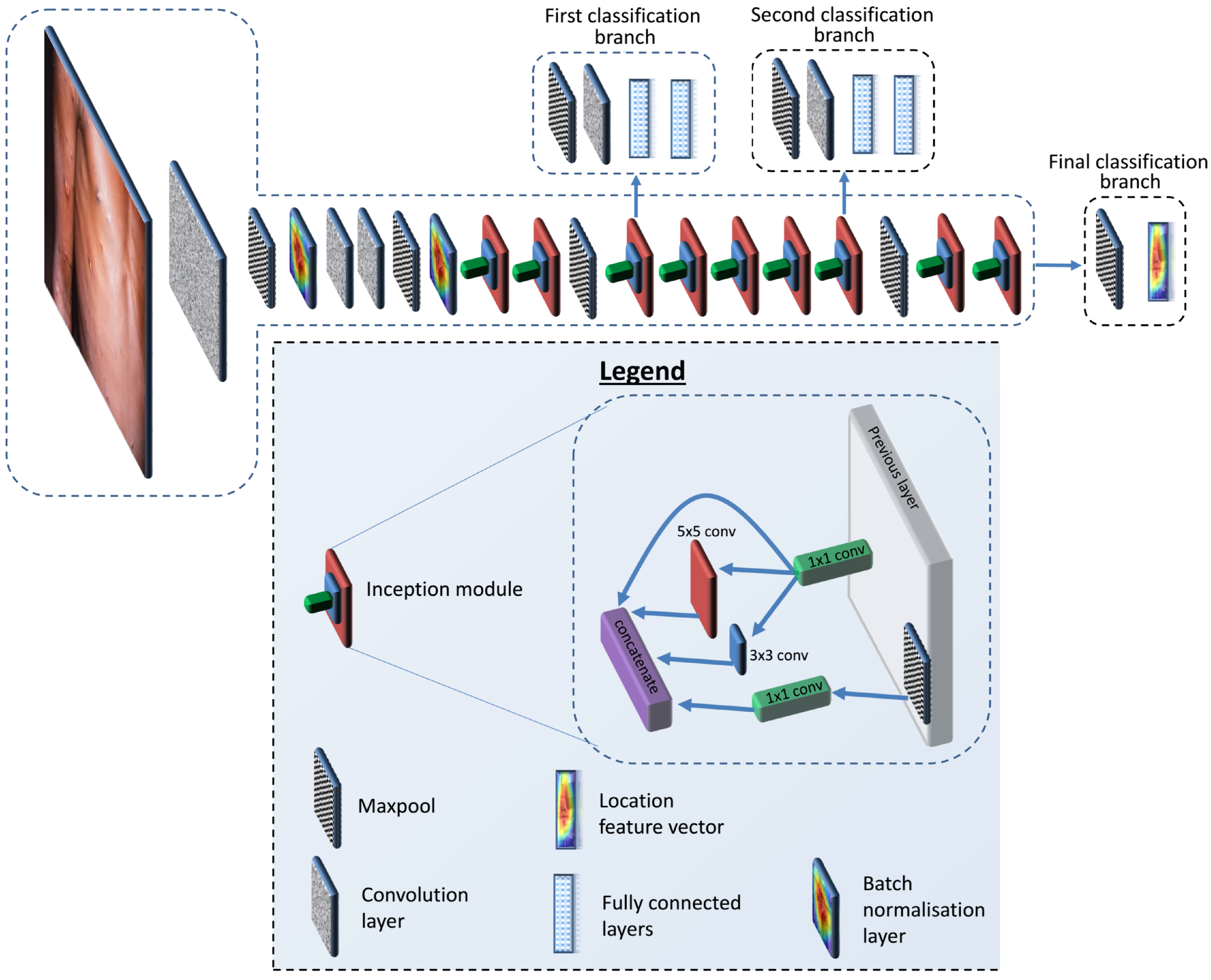
3.1.4. GoogleNet Deep Network

GoogLeNet and the rest of the Inception model deep learning family are built on iterations of an Inception module [39]. Using a network-within-a-network strategy, the Inception module does its best to approximate the convolutional vision network’s local sparse structure. GoogLeNet, a model developed by Google, achieved top-5 error accuracy of 6.67%, making it the winner of the ILSVRC 2014 competition. Inception versions 1–4 and Inception–ResNet are two variants of GoogLeNet that may be accessed by the general public. As a network inside a network, Inception has a spatial repetition of the best local sparse structure of a visual network. Inception uses 11 inexpensive convolutions to compute reductions before resorting to the 33 or 55 more resource-intensive convolutions. An example of a high-capability architecture that served as a model for our own design is GoogleNet. New concepts, algorithms, and enhanced network topologies are just as important as more processing power, larger datasets, and more complex models when it comes to improving identification capabilities. The architecture of the GoogleNet deep network is shown in Figure 1. In this work, the GoogleNet deep network was adopted for feature extraction based on the results achieved compared to those of other deep networks.

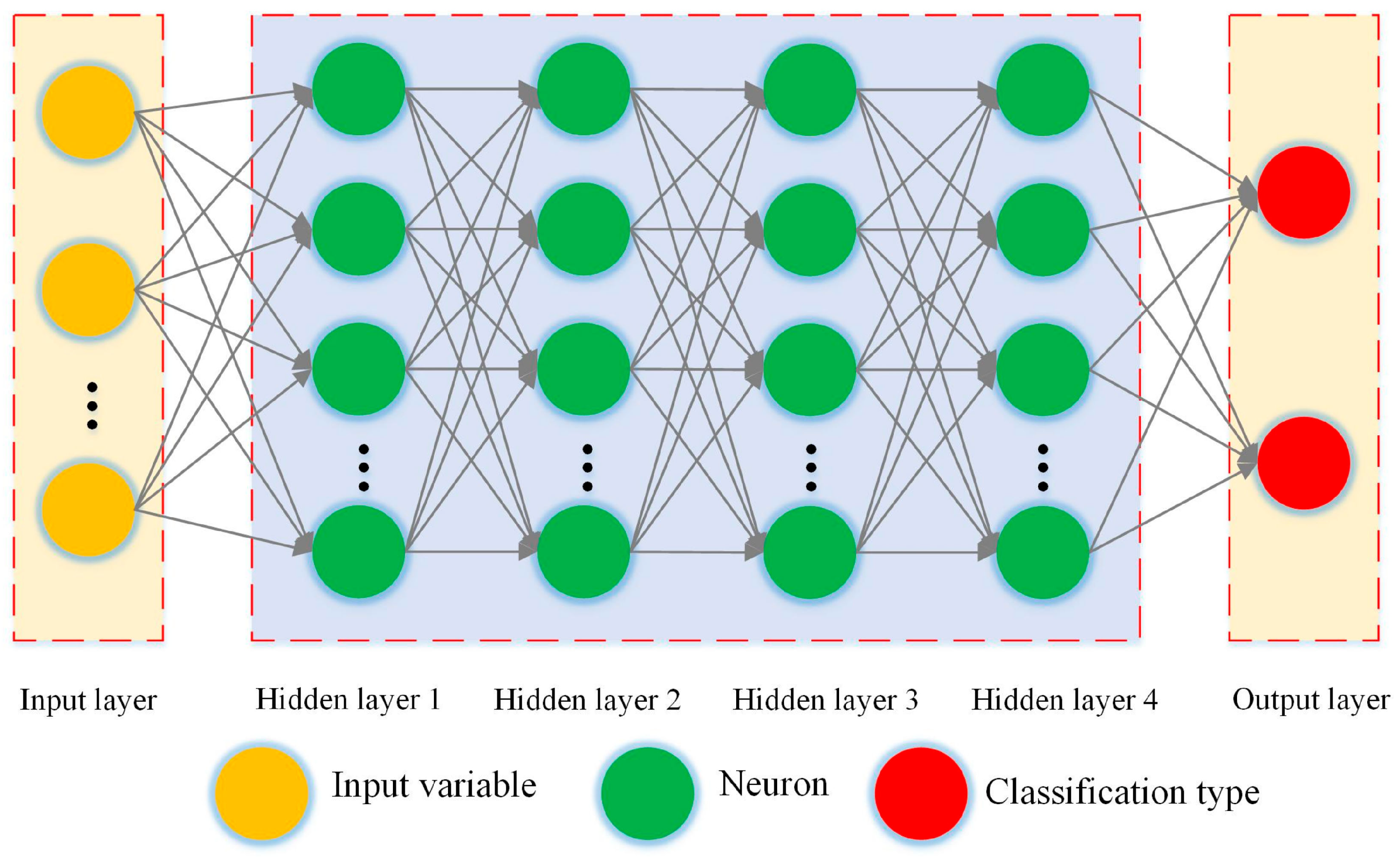
3.2. Multi-Layer Neural Network

In the neural network (NN) model known as the multi-layer perceptron [40], the neurons in the interstitial spaces between the several hidden layers are interconnected [41]. Figure 2 depicts the model architecture of the developed NN employed for classifying the selected features of the input images. The developed NN makes use of both practice and experimentation in its parameter selection. The parameters of this NN are optimized using the proposed meta-heuristic optimization algorithm. The details of the optimization algorithm and the optimized parameters are presented and discussed in the next sections.

3.3. Meta-Heuristic Optimization

In this paper, three optimization algorithms, namely, Al-Biruni Earth radius (BER), the sine cosine algorithm (SCA), and particle swarm optimization (PSO), were utilized. These algorithms were used to develop two new hybrid optimization algorithms for feature selection and NN parameter optimization. In this section, the basics of these algorithms are presented; then, the proposed hybrid optimization algorithms are explained in the next section.

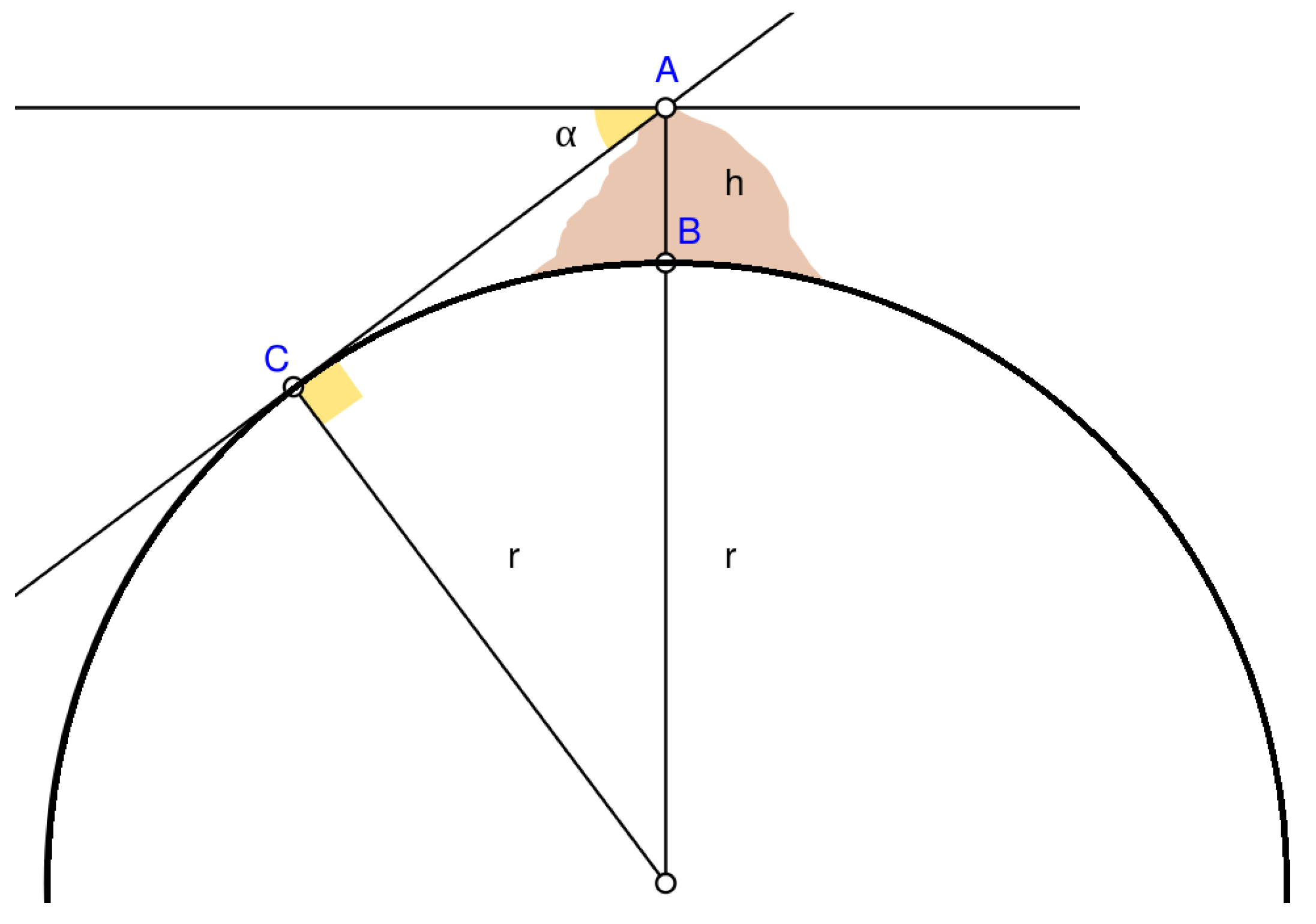
3.3.1. Al-Biruni Earth Radius (BER) Optimization Algorithm

The calculation of earth radius based on Al-Biruni method is depicted in Figure 3. This method forms the basis of Al-Biruni Earth Radius (BER) optimization algorithm. Finding the optimal solution within specified constraints is the work of optimization algorithms. Each member of the population can be represented by a S vector in the BER algorithm: $S=S_1,S_2,\dots ,S_d\in R$, where $S_d$ is the dimension of the search space and d is the dimension of the parameter or feature being optimized. It is proposed that success up to some limit be measured using the fitness function F. Using these stages of the optimization procedure, populations may be searched for a fitness-maximizing vector $S^{*}$. To begin, a sample of the population is chosen at random (solutions). Before BER can begin optimizing, a number of factors must be specified, including the fitness function, the minimum and maximum allowed solution sizes, the population size, the dimensions, and the number of solutions. Exploration and exploitation operations form the backbone of the BER algorithm as explained in the following.

• Exploration Operation: This operation is responsible for locating promising areas of the search space and breaking through local optimum stasis on the way to the best possible solution.

  –

  Moving towards the best solution: Using this strategy, the solitary explorer will scout out the immediate region around its current location for potentially fruitful new exploration sites. One way to accomplish this is by using an iterative process to search for a more optimal option (with respect to fitness) from the numerous available choices nearby. BER analysis uses the following formulas to accomplish this goal:

  $$r=h\frac{cos\left(x\right)}{1-cos\left(x\right)}$$

  (1)

  $$D=r_1(S\left(t\right)-1)$$

  (2)

  $$S(t+1)=S\left(t\right)+D(2r_2-1)$$

  (3)

  where $0<x\le 180$, h is a number that is randomly selected from the range $[0,2]$, $r_1$ and $r_2$ are coefficient vectors whose values are measured by Equation (1), $S\left(t\right)$ is the solution vector at iteration t, and D is the diameter of the circle in which the search agent will look for promising areas.

• Exploitation Operation: The exploiting group is accountable for improving current solutions. When a cycle ends, the BER calculates the fitness of each participant and awards those with the best scores. The BER employs two unique strategies to achieve the aim of exploitation, both of which are outlined in the following.

  –

  Moving towards the best solution: The following equation is employed to move in the direction of the best solution.

  $$S(t+1)=r^2(S\left(t\right)+D)$$

  (4)

  $$D=r_3(L\left(t\right)-S\left(t\right))$$

  (5)

  where $r_3$ is a random vector calculated using Equation (2) that controls the movement steps towards the best solution, $S\left(t\right)$ is the solution vector at iteration t, $L\left(t\right)$ is the best solution vector, and D refers to the distance vector.

  –

  Searching the area around the best solution Generally speaking, the region around the optimal response offers the most potential for success (leader). As a result, some people will hunt for ways to enhance the situation by investigating alternatives that are somewhat similar to the best one. To implement the aforementioned process, BER employs the following equation.

  $$S^{\prime }(t+1)=r(S^{*}\left(t\right)+k)$$

  (6)

  $$k=1+\frac{2\times t^2}{Ma{x}_{iter}^2}$$

  (7)

  where the best solution is denoted bu $S^{*}\left(t\right)$, which is selected after comparing $S(t+1)$ and $S^{\prime }(t+1)$. The following equation is used to mutate the solution if the best fitness was not changed in the last two iterations.

  $$S(t+1)=k\ast z^2-h\frac{cos\left(x\right)}{1-cos\left(x\right)}$$

  (8)

  where z is a random number in the range $[0,1]$ and t is the iteration number.

• Selection of the best solution: To ensure that the solutions are of excellent quality, the BER chooses the best ones to employ in the next cycle. While the elitism technique is more effective, it may lead multi-modal functions to converge too soon [42,43]. By taking a mutational approach and scanning the area surrounding the explorers, the BER is able to deliver cutting-edge exploration capabilities. With its robust exploration capabilities, the BER is able to stave off convergence. First, parameters such as population size, mutation frequency, and iteration count are input into the BER. The BER then assigns individuals to either the exploration group or the exploitation group. The BER method dynamically modifies the size of each group throughout the iterative process of locating the best solution. Two approaches are used by each group to complete their missions. The BER ensures diversity and thorough exploration by shuffling the order of responses between repetitions. In one iteration, a solution may be part of the exploration group, but by the next, it may be part of the exploitation group. Due to the BER’s exclusive nature, the leader will not be deposed during the procedure.

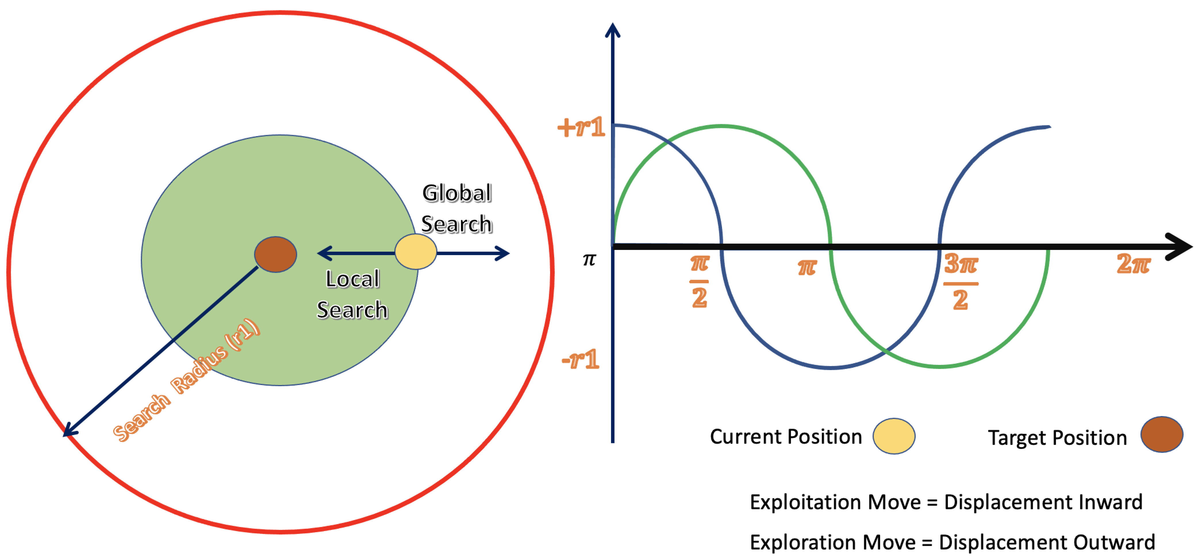
3.3.2. Sine Cosine Algorithm

The sine cosine algorithm (SCA) was initially introduced in [44]. Based on Figure 4, it can be noted that the oscillation functions of sines (and cosines) have an important role in determining the optimal solution sites. To express the operations of SCA, a collection of random variables is employed [45].

• The motion direction.
• The movement location.
• Emphasizing/de-emphasizing the destination effect.
• Swapping between the sine and cosine components.

The update process of the candidate solutions is performed using the following equation.

$$P(t+1)=\left\{\begin{array}{cc}P\left(t\right)+r_5·sin\left(r_6\right)·|r_7{S}^{*}\left(t\right)-S\left(t\right)|\hfill & r_4<0.5\hfill \\ P\left(t\right)+r_5·cos\left(r_6\right)·|r_7{S}^{*}\left(t\right)-S\left(t\right)|\hfill & r_4\ge 0.5\hfill \end{array}\right.$$

(9)

in which t is the number of search iterations. Current and best solutions are referred to as S and $S^{*}$. The values of $[0-1]$ are allocated to the random variables $r_4$, $r_6$, and $r_7$. For example, as can be seen from the equation, the locations of the best solutions influence the present solution’s position, making it easier to get to an ideal solution. The value of $r_4$ is changed as follows during the running iterations of SCA.

$$r_4=a-\frac{a\times t}{t_{max}}$$

(10)

where a is a constant, and t and $t_{max}$ represent the current and maximum iterations, respectively.

The SCA algorithm is more resilient than a broad range of meta-heuristic approaches in the literature because it uses just one optimal solution to lead the other solutions. Compared to other algorithms, this algorithm’s convergence speed and memory usage are quite low [45]. Nevertheless, as the number of local optimum solutions grows, the algorithm’s efficiency declines. Since the local optima can become stagnant, the SCA optimizer and the GWO algorithm are incorporated into the proposed algorithm to take advantage of their fast convergence rates and memory efficiency, and to ensure a healthy ratio of exploration to exploitation tasks during the optimization process.

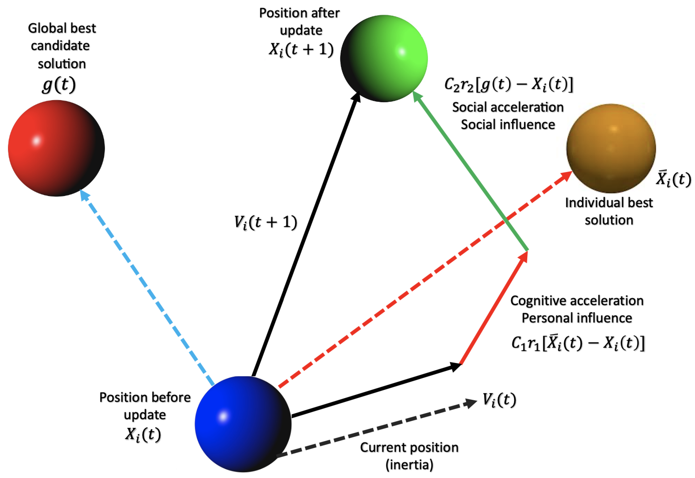
3.3.3. Particle Swarm Optimization

The particle swarm optimization (PSO) methodology is based on mimicking the foraging behavior of flocking animals such as birds using an optimization tool that outperforms the group intelligence approach. Some technical optimization issues can be solved with the PSO method, which was developed after observing this class of animal foraging patterns. All particles in the PSO algorithm have an adjustable value, and their search velocity and range are controlled by the speed at which they move, as shown in Figure 5. Particles then conduct their solution space search from the optimal particle’s position in the population. Particles keep themselves current during the search process by monitoring two extreme values: the individual extremum $P_{best}$, which is the optimal solution discovered by an individual particle, and the global extremum $g_{best}$, which is the ideal solution currently found by the whole group. A scenario where the particles are looked for in a D-dimensional target space is considered, where a group of N particles live together. The i-th particle’s velocity throughout its journey is a D-dimensional vector:

$$V_i=(V_{i1},V_{i2},\dots ,V_{iD}),i=1,2,\dots ,N$$

(11)

Each particle’s particular extremum, defined as its best possible position in the solution space, is represented by the notation:

$$P_{best}=P_{i1},P_{i2},\dots ,P_{iD},i=1,2,\dots ,N$$

(12)

As long as the particle locates both the local and global extrema, it can modify its current velocity and position using the following formulas.

$$V_{id}(t+1)=w\ast V_{id}\left(t\right)+c_1{r}_1(P_b-P_{id}\left(t\right))+c_2{r}_2(P^{*}-P_{id}\left(t\right))$$

(13)

$$P_{id}(t+1)=P_{id}\left(t\right)+V_{id}(t+1)$$

(14)

where the global extremum is denoted by $P^{*}$, w refers to the inertia weight, and the learning factors $c_1$ and $c_2$ are selected arbitrarily in the range between 0 and 2. $V_{im}$ refers to the particle velocity, and $r_1$ and $r_2$ are random numbers between 0 and 1.

4. The Proposed Methodology

In this section, two proposed hybrid optimization algorithms are explained for improving the feature selection optimization of NN parameters. The first algorithm is based on particle swarm optimization and Al-Biruni Earth radius optimization algorithms and is referred to as PSOBER. The binary version of this algorithm is used for feature selection. The second algorithm is based on the sine cosine algorithm (SCA) and the Al-Biruni Earth radius (BER) optimization algorithm and is referred to as SCBER. The proposed algorithms exploit the advantages of both algorithms they use for better selection of the best solution.

Figure 6 depicts the stages of the proposed approach. As shown in the figure, the first stage is the data processing, which includes image resizing, data augmentation, and feature extraction. This stage focuses on preparing the input images and increasing the number of images, and then extracting the relevant features using GoogleNet. The second stage, on the other hand, is the feature selection, which involved the proposed feature selection algorithm. The target of this stage is to select the most effective features that can accuracy classify the input images. The advantage of this stage is that is reduces the number of features extracted by the deep learning by excluding the irrelevant features. Finally, the third stage is the optimization of the neural network’s parameters using the proposed optimization algorithm. The target of this step is to choose the best set of parameters for classification. The following sections discuss the details of the proposed feature selection and parameter optimization algorithms.

4.1. The Proposed PSOBER Optimization Algorithm

The feature selection process employed in this work is based on the proposed hybrid particle swarm optimization (PSO) algorithm and Al-Biruni Earth radius (BER) optimization algorithm, and it is denoted by PSOBER. The steps of PSOBER are presented in Algorithm 1. In this algorithm, the collaboration between the BER and PSO algorithms finds the best solutions. During the search process, the BER algorithm operates in even-number iterations. The PSO algorithm works in odd-number iterations, as presented in Line 5 of the algorithm. This interchanging operation of the BER and PSO allows for better exploration and exploitation of the search process. The achieved results, explained in the next section, confirm this achievement.

Algorithm 1 The PSOBER optimization algorithm.

1: Initialize PSOBER population $P_i(i=1,2,\dots ,d)$, $V_i(i=1,2,\dots ,d)$ with size d, iterations $Ma{x}_{iter}$, fitness function $F_n$, $t=1$, $n_1$, $n_2$, $r_1$, $r_2$, $r_3$, $r_4$, $r_5$, $c_1$, $c_2$ 2: Calculate fitness function $F_n$ for each $P_i$ 3: Find best solution as $P^{*}$ 4: while $t\le Ma{x}_{iter}$ do 5:    if t%2 == 0 then 6:      for ($i=1:i<n_1+1$) do 7:         Update $r=h\frac{cos\left(x\right)}{1-cos\left(x\right)}$ 8:         Calculate $D=r_1(P\left(t\right)-1)$ 9:         Update positions to head toward best solution as         $P(t+1)=P\left(t\right)+D(2r_2-1)$ 10:      end for 11:      for ($i=1:i<n_2+1$) do 12:         Calculate $D=r_3(L\left(t\right)-P\left(t\right))$ 13:         Update positions of best solution as         $P(t+1)=r_2(P\left(t\right)+D)$ 14:         Calculate $k=1+\frac{2\times t^2}{Ma{x}_{iter}^2}$ 15:         Investigate area around best solution as         $P^{\prime }(t+1)=r_1(P^{*}\left(t\right)+k)$ 16:         Compare $P(t+1)$ and $P^{\prime }(t+1)$ to select best solution $P^{*}$ 17:         if best fitness is not changed for last two iterations then 18:           Mutate solution as $P(t+1)=k*z^2-h\frac{cos\left(x\right)}{1-cos\left(x\right)}$ 19:         end if 20:      end for 21:    else 22:      for each particle $i=1,\dots ,N$ do 23:         for each dimension $d=1,\dots ,n$ do 24:           Update the particle’s velocity using:           $V_{id}(t+1)=w{V}_{id}+c_1{r}_1(P_{id}-P_{id}\left(t\right))+c_2{r}_2(P^{*}-P_{id}\left(t\right))$ 25:           Update the particle’s position using:           $P_{id}(t+1)=P_{id}\left(t\right)+V_{id}(t+1)$ 26:         end for 27:      end for 28:    end if 29:    Update the fitness function $F_n$ for each $P_i$ 30:    Update BER parameters, $t=t+1$ 31: end while 32: Return $P^{*}$

4.2. The Proposed Binary PSOBER Optimization Algorithm

In order to determine whether or not a given feature is important, feature selection problems have a small search space consisting only of the binary values 0 and 1. Consequently, the binary PSOBER method is proposed in this part, which transforms the continuous values produced by the continuous PSOBER algorithm into binary [0, 1] to conform to the feature selection procedure. The primary function of this algorithm is to convert the continuous solution into a binary solution in terms of the following $Sigmoid$ function.

$$\begin{array}{cc}\hfill & P_t^{*}=\left\{\begin{array}{cc}1\hfill & \mathrm{if}Sigmoid\left(P_t^{*}\right)\ge 0.5\hfill \\ 0\hfill & otherwise\hfill \end{array}\right.,\hfill \\ \hfill & Sigmoid\left(P_t^{*}\right)={\displaystyle \frac{1}{1+e^{-10(P_t^{*}-0.5)}}}\hfill \end{array}$$

(15)

where $P_t^{*}$ denotes the optimal solution at step t. Algorithm 2 details the steps of the proposed binary PSOBER used in selecting the best set of features that can boost the classification accuracy of monkeypox cases.

Algorithm 2 The proposed binary PSOBER algorithm.

1: Initialize Set PSOBER population, parameters, configuration. 2: Convert solutions to binary [0, 1]. 3: Calculate objective function and select best solutions. 4: Train k-NN and calculate error 5: while $t\le Ma{x}_{iter}$ do 6:    Find the best solution using PSOBER algorithm 7:    Convert solutions to binary using Equation (15) 8:    Calculate Fitness 9:    Update Positions 10: end while 11: Return $X^{*}$

Objective Function

With the help of the following formula representing the objective function, it is possible to evaluate the accuracy of the solution generated by the proposed optimization method.

$$F_t=\alpha Error\left(Params\right)+\beta \frac{\left|A\right|}{\left|B\right|}$$

(16)

where $Params$ stands for the model’s input parameters. The significance of the chosen traits in the population is reflected by the values of $alpha\in$ [0, 1] and $beta=1-alpha$. While $\left|A\right|$ represents the number of features that were used to make a decision, $\left|B\right|$ represents the total number of features in the dataset. The optimal strategy is one that uses as few features as possible to get a high-quality classification.

4.3. The Proposed SCBER Optimization Algorithm

To achieve better classification performance, an optimization algorithm is proposed based on a hybrid between the sine cosine and Al-Biruni Earth radius optimization algorithms, which is denoted by SCBER. This optimization algorithm is used to optimize the parameters of a multi-layer neural network. The steps of the proposed SCBER algorithm are listed in Algorithm 3.

When applied to a population, the proposed SCBER algorithm strikes an automated balance between exploring and exploiting different segments of the population. In the proposed method, 70% of the population is divided into two groups: exploration and exploitation. Having a large number of individuals involved in the exploration group helps with finding new and intriguing search regions. Individual fitness increases when more opportunistic individuals are able to increase their fitness levels, but the percentage of individuals in the exploratory group rapidly decreases from 70% to 30%. If a better solution cannot be identified, then using an elitism approach guarantees convergence by keeping the process leader in subsequent populations. SCBER may increase the size of the exploration group at any point so long as the leader’s fitness has not increased sufficiently throughout three iterations.

Algorithm 3 The proposed SCBER optimization algorithm.

1: Initialize BER population $P_i(i=1,2,\dots ,d)$ with size d, iterations $Ma{x}_{iter}$, fitness function $F_n$, $t=1$, $n_1$, $n_2$, a, $r_1$, $r_2$, $r_3$, $r_4$, $r_5$, $r_6$, $r_7$ 2: Calculate fitness function $F_n$ for each $P_i$ 3: Find best solution as $P^{*}$ 4: while $t\le Ma{x}_{iter}$ do 5:    if t%2 == 0 then 6:      for ($i=1:i<n_1+1$) do 7:         Update $r=h\frac{cos\left(x\right)}{1-cos\left(x\right)}$ 8:         Calculate $D=r_1(P\left(t\right)-1)$ 9:         Update positions to head toward best solution as         $P(t+1)=P\left(t\right)+D(2r_2-1)$ 10:      end for 11:      for ($i=1:i<n_2+1$) do 12:         Calculate $D=r_3(L\left(t\right)-P\left(t\right))$ 13:         Update positions of best solution as         $P(t+1)=r_2(P\left(t\right)+D)$ 14:         Calculate $k=1+\frac{2\times t^2}{Ma{x}_{iter}^2}$ 15:         Investigate area around best solution as         $P^{\prime }(t+1)=r_1(P^{*}\left(t\right)+k)$ 16:         Compare $P(t+1)$ and $P^{\prime }(t+1)$ to select best solution $P^{*}$ 17:         if best fitness is not changed for last two iterations then 18:           Mutate solution as $P(t+1)=k*z^2-h\frac{cos\left(x\right)}{1-cos\left(x\right)}$ 19:         end if 20:      end for 21:    else 22:      Update current birds’ positions as 23:      if $r_4<0.5$ then 24:         Update birds’ positions by $P(t+1)=P\left(t\right)+r_5\times sin\left(r_6\right)\times |r_7{P}^{*}\left(t\right)-P\left(t\right)|$ 25:      else 26:         Update birds’ positions by $P(t+1)=P\left(t\right)+r_5\times cos\left(r_6\right)\times |r_7{P}^{*}\left(t\right)-P\left(t\right)|$ 27:      end if 28:      Calculate $r_4=a-\frac{a\times t}{t_{max}}$ 29:    end if 30:    Update the fitness function $F_n$ for each ${\mathbf{P}}_i$ 31:    Update BER parameters, $t=t+1$ 32: end while 33: Return $P^{*}$

5. Experimental Results

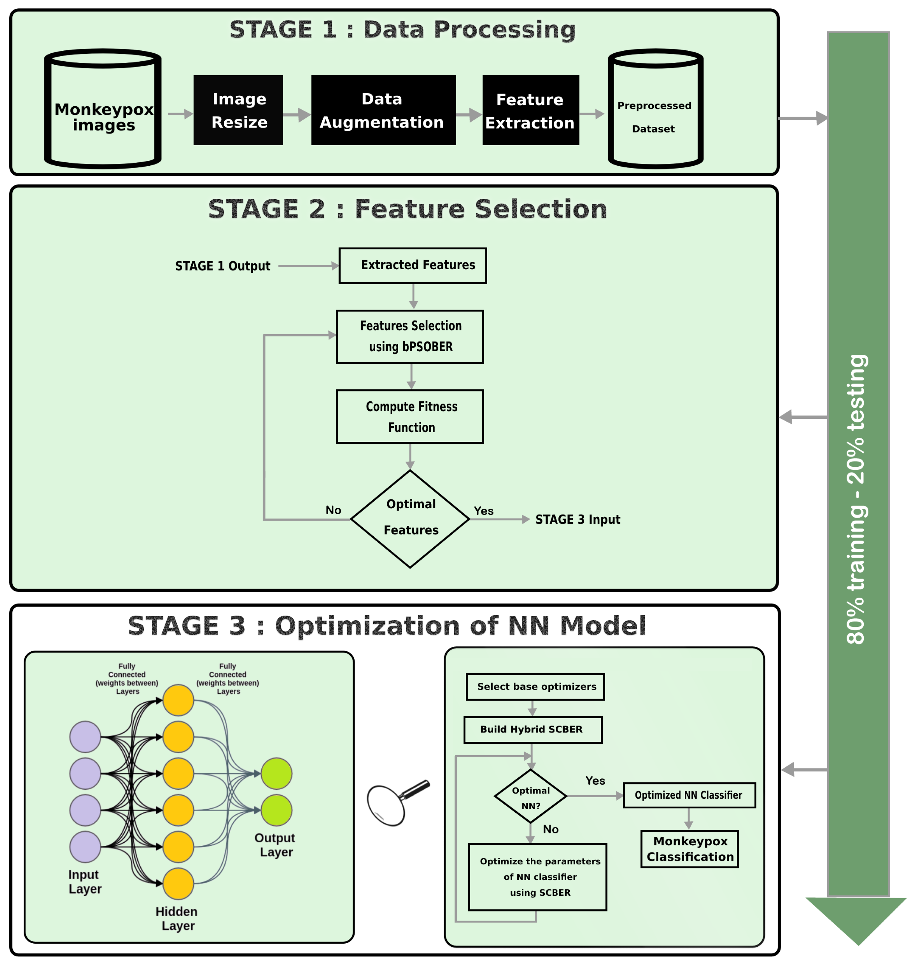
Three sets of experiments were carried out in this paper to evaluate the proposed algorithms. The purpose of the first set of experiments was to determine which of the deep learning networks available for feature extraction performs the best, and then adopt the best performing deep network. The results of the best-adopted network werer then fed to the proposed feature selection algorithm (bPSOBER), which was evaluated using the second set of experiments. The selected features were classified using the optimized NN, which was optimized using the proposed SCBER, which was evaluated using the third set of experiments. In addition, a set of statistical experiments were conducted to assess the stability and significance of the proposed algorithms. In this section, the results of these experiments are presented and explained.

The hardware parameters of the platform that ran the experiments were: central processing unit (CPU) of type Intel Core i7, the graphics processing unit (GPU) was GeForce RTX2070 Super with 8 GB memory, and the main memory was of size 16 GB. On the other hand, the software parameters were: platform was Ubuntu 20.04 with CUDA9.0, Cudnn7.1, TensorFlow 1.15, and Spider IDE with Python3.7. Based on these parameters, the experiments were conducted in ≥16 batches, which enabled completing the model training process in a relatively short time.

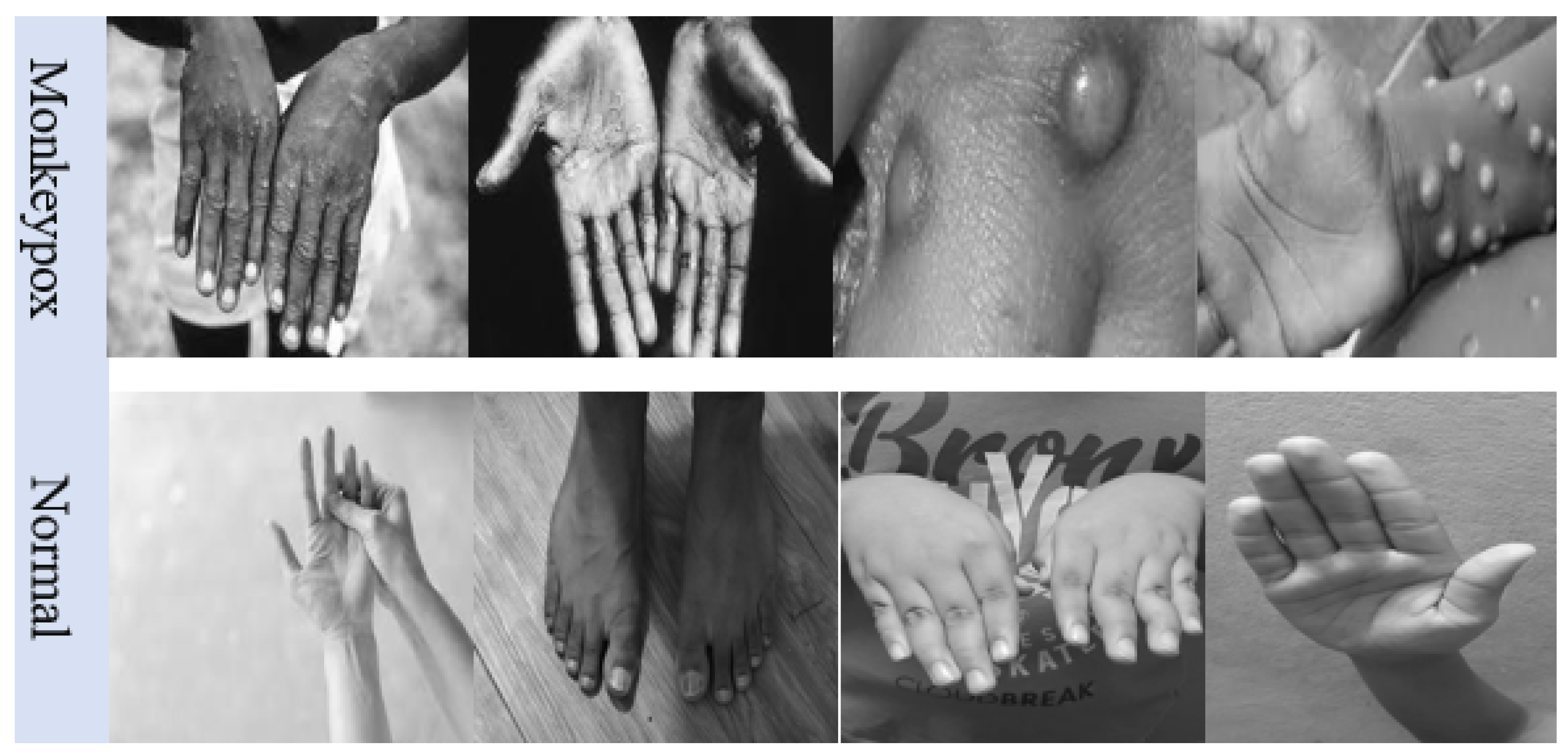
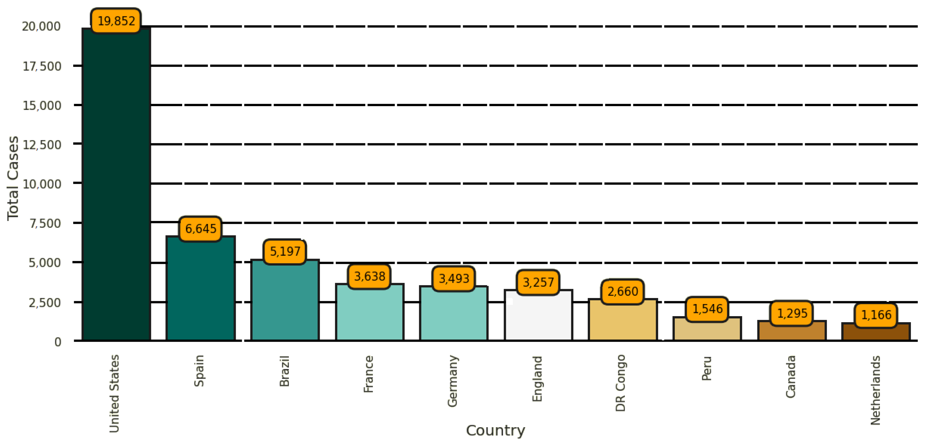
5.1. Monkeypox Dataset

The experiments conducted in this work were based on a freely available dataset on Kaggle [46]. This dataset is composed of 279 images of monkeypox cases and 293 images of normal cases. Sample images of the dataset are shown in Figure 7, and the spread of the contamination of the monkeypox infection is shown in Figure 8. As the size of the dataset is small, data augmentation was applied to increase the number of images in the dataset to enable transfer learning for feature extraction.

5.2. Evaluation Criteria

The effectiveness of the proposed feature selection procedure is evaluated in terms of the metrics presented in

Table 1. The metrics used in evaluating the performance of the proposed feature selection method.

Metric	Value
Mean	$\frac{1}{M}{\sum }_{i=1}^M{P}_{*}^i$
Worst fitness	$ma{x}_{i=1}^M{P}_{*}^i$
Best fitness	$mi{n}_{i=1}^M{P}_{*}^i$
Average fitness size	$\frac{1}{M}{\sum }_{i=1}^{M}size\left(P_{*}^i\right)$
Standard deviation	$\sqrt{\frac{1}{M-1}{\sum }_{i=1}^M{\left(P_{*}^i-Mean\right)}^2}$
Average error	$\frac{1}{M}{\sum }_{j=1}^M\frac{1}{N}{\sum }_{i=1}^{N}mse(C_i,L_i)$

. These metrics include mean, worst fitness, best fitness, average fitness size, standard deviation, and average error. On the other hand, the effectiveness of the extracted features and the performance of the proposed optimized neural network are evaluated in terms of the metrics listed in

Table 2. The metrics used in evaluating the performance of the proposed optimized NN.

Metric	Value
Accuracy	$\frac{TP+TN}{TP+TN+FP+FN}$
Nvalue (NPV)	$\frac{TN}{TN+FN}$
Pvalue (PPV)	$\frac{TP}{TP+FP}$
Sensitivity (TPR)	$\frac{TP}{TP+FN}$
Specificity (TNR)	$\frac{TN}{TN+FP}$
F1-Score	$\frac{TP}{TP+0.5(FP+FN)}$

. These metrics include accuracy, n-value, p-value, sensitivity, specificity, and F1-score. In these tables, M represents the total number of optimization iterations, $P_j^{*}$ stands for the best solution vector at iteration j, and $size(P_j^{*})$ indicates the size of the best solution. The number of data points in the test set is represented by N, and the output label at data point i is marked by $C_i$. The number of features is denoted by D, and the label of the class of point i is denoted by $Li$. True positive, false positive, and false negative are abbreviated as $TP$, $TN$, $FP$, and $FN$, respectively [47].

5.3. Configuration Parameters

Table 3. Configuration parameters of the proposed algorithms.

Parameter	Value
Population size	30
Number of iterations	100
Mutation probability	0.5
K (decreases from 2 to 0)	1
Inertia factor of SCA	0.1
Exploration percentage	70
Number of runs	30
Number of agents	20
Dimension	Features count
$\alpha$ of Equation (16)	0.99
$\beta$ of Equation (16)	0.01

displays the proposed algorithms’ configuration parameters. These parameters include the population size, number of training iterations, mutation probability, and K factor for the BER parts of the proposed algorithms; the inertial factor of the SC algorithm; the exploration percentage; the numbers of runs and agents; the dimensions of the search space; and finally, the values of $\alpha$ and $\beta$, which were set as 0.99 and 0.01, respectively. On the other hand,

Table 4. Configuration parameters of the competing algorithms.

Algorithm	Parameter	Value
SC	Inertia factor	0.1
	Iterations	100
	Runs	30
FA	Iterations	80
	Fireflies	10
GA	Cross over	0.9
	Mutation ratio	0.1
	Selection mechanism	Roulette wheel
	Iterations	80
	Agents	10
PSO	Acceleration constants	[2, 12]
	Inertia $W_{min}$, $W_{max}$	[0.6, 0.9]
	Iterations	80
	Particles	10
WOA	r	[0, 1]
	a	2 to 0
	Iterations	80
	Whales	10
GWO	a	2 to 0
	Wolves	10
	Iterations	80

displays the settings for the other competing algorithms used in the experiments.

5.4. Stage 1: Preprocessing Results

The preprocessing of the input dataset was applied through a set of steps, including resizing the input images, data augmentation, evaluation of the given deep networks to chose the best, and then feature extraction.

5.4.1. Data Augmentation

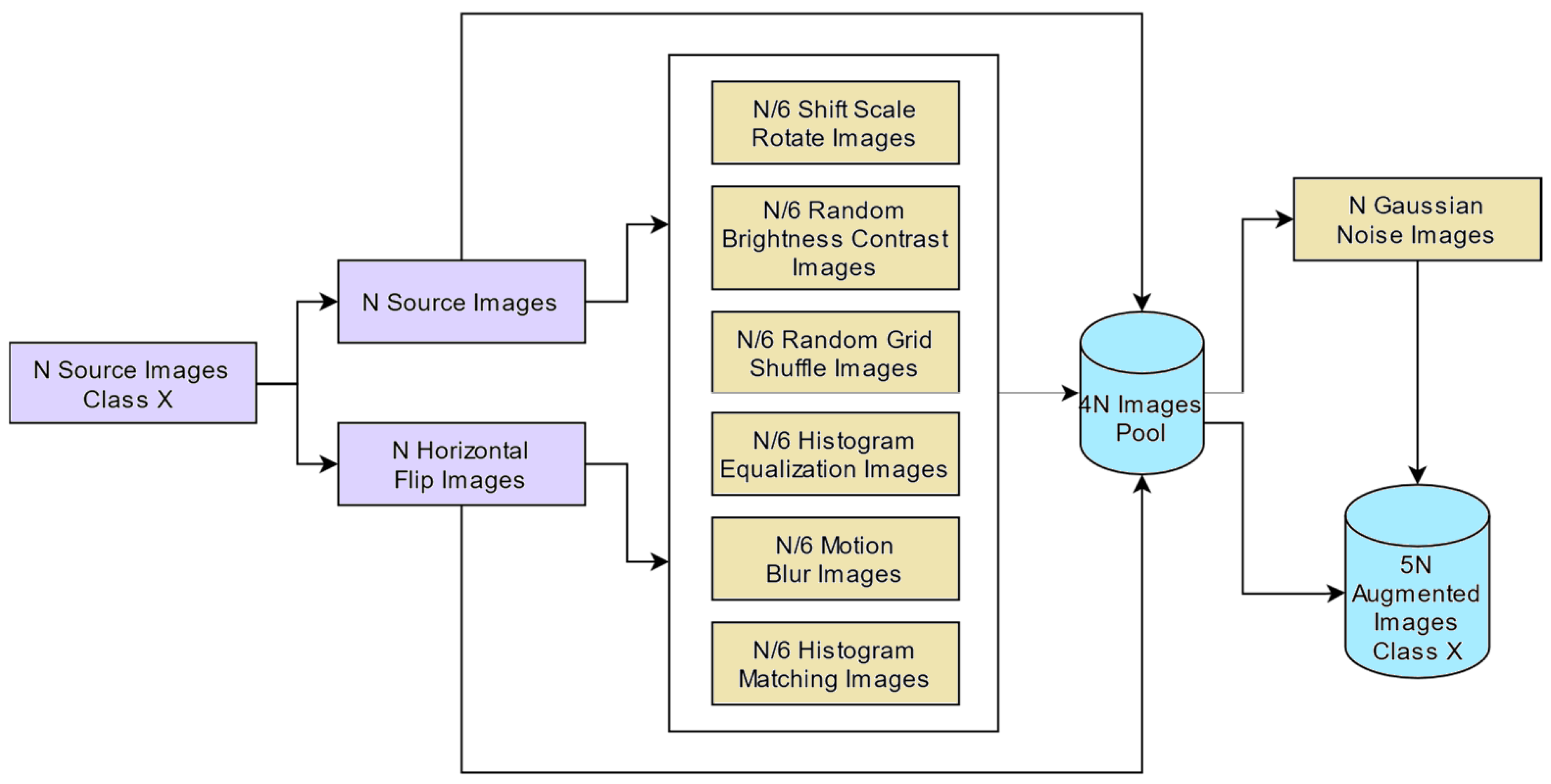
The term “data augmentation” refers to the method of changing the size and orientation of the dataset images to generate new image that can enrich the existing dataset. Data augmentation is used on both training and validation sets to boost the generalization capacity of deep learning-based image classification models. Various data augmentation techniques, such as geometric modification, kernel filters, picture mixing, random erasure, and transformations, were applied to increase the size of the dataset. The image augmentation pipeline was developed for monkeypox images using some selected augmentation methods. All images in the validation and training sets for each class were scaled to $224\times 224$ before being augmented. The process of image augmentation is depicted in Figure 9.

5.4.2. Evaluating the Deep Learning Networks

Machine-learning models rely heavily on the detection and extraction of key features from input images. Here, the outputs of four different deep neural networks, namely, AlexNet [36], VGG-19 [37], GoogleNet [39], and ResNet-50 [38], are compared based the same dataset. The outputs from these networks are presented in

Table 5. Evaluation of the features extracted using four deep neural networks and the developed multi-layer neural network.

Metric	AlexNet	VGG19Net	ResNet-50	GoogLeNet
Accuracy	0.84	0.86	0.88	0.89
Sensitivity (TPR)	0.63	0.63	0.63	0.63
Specificity (TNR)	0.90	0.93	0.96	0.98
Pvalue (PPV)	0.66	0.73	0.85	0.91
Nvalue (NPV)	0.89	0.89	0.89	0.89
F-score	0.64	0.67	0.72	0.74

. Using the default parameters, we first gathered the features of the images from the preceding layers of a deep neural network so that they could be used in the subsequent operations for feature selection and balancing. GoogleNet had the best performance, as seen in the results. Therefore, this was adopted by extracting the features that were then fed to the feature selection process.

5.5. Stage 2: Feature Selection Results

The selection of the most significant features of the features extracted by GoogleNet was essential. In this experiment, six optimization methods were employed—namely, the bPSOBER, binary BER (bBER), binary particle swarm optimizer (bPSO) [48], binary whale optimization algorithm (bWOA) [49], binary gray wolf optimizer (bGWO) [50], binary firefly algorithm (bFA) [51], and binary genetic algorithm (bGA) [52]. The evaluation of results achieved by these feature selection methods is listed in

Table 6. Evaluation of the proposed feature selection algorithm (bPSOBER) compared to other competing methods.

	bPSOBER	bBER	bPSO	bWAO	bGWO	bFA	bGA
Average error	0.83508	0.85228	0.88608	0.88588	0.87238	0.88448	0.86588
Average Select size	0.78788	0.98788	0.98788	1.15128	0.91068	1.02238	0.93028
Average Fitness	0.89828	0.91448	0.91288	0.92068	0.92058	0.96478	0.92588
Best Fitness	0.80008	0.83478	0.89318	0.88478	0.89838	0.88348	0.82918
Worst Fitness	0.89858	0.90168	0.96088	0.96088	0.97458	0.98108	0.94428
Standard deviation Fitness	0.72058	0.72528	0.72468	0.72688	0.72588	0.76148	0.72688

. It can be seen in this table that the results achieved by the proposed bPSOBER algorithm are superior to those achieved by the other feature selection methods.

To demonstrate that the proposed feature selection algorithm (bPSOBER) is statistically significantly superior, the p-values were computed by comparing the outputs of each pair of algorithms. To conduct this study, Wilcoxon’s rank-sum test was employed. There are two major hypotheses at play here: the null and the alternative. The mean ($\mu$) values of the null hypothesis represented by $H0$ include $\mu bPSOBER=\mu bBER$, $\mu bPSOBER=\mu bPSO$, $\mu bPSOBER=\mu bWOA$, $\mu bPSOBER=\mu bGWO$, $\mu bPSOBER=\mu FA,$ and $\mu bPSOBER=\mu bGA$. However, the $H1$ hypothesis does not factor in the averages of the algorithms. The outcomes of the Wilcoxon rank-sum test are shown in

Table 7. The Wilcoxon signed-rank test for evaluating the the proposed feature selection algorithm (bPSOBER) compared to other competing feature selection methods.

	bPSOBER	bBER	bPSO	bWAO	bGWO	bSC	bGA
Theoretical median	0	0	0	0	0	0	0
Actual median	0.8351	0.8523	0.8861	0.8859	0.8724	0.8845	0.8659
Number of values	14	14	14	14	14	14	14
Wilcoxon Signed Rank Test
Sum of signed ranks (W)	105	105	105	105	105	105	105
Sum of positive ranks	105	105	105	105	105	105	105
Sum of negative ranks	0	0	0	0	0	0	0
P value (two tailed)	0.0001	0.0001	0.0001	0.0001	0.0001	0.0001	0.0001
Exact or estimate?	Exact	Exact	Exact	Exact	Exact	Exact	Exact
Significant (alpha = 0.05)?	Yes	Yes	Yes	Yes	Yes	Yes	Yes
How big is the discrepancy?
Discrepancy	0.8351	0.8523	0.8861	0.8859	0.8724	0.8845	0.8659

. Compared to the previous algorithms, the suggested one has a lower p-value (p < 0.005). The suggested feature selection approach was validated by these findings, demonstrating its statistical superiority. A one-way analysis of variance (ANOVA) test was performed to examine whether or not there were statistically significant differences between the suggested bPSOBER algorithm and the other algorithms. The mean ($\mu$) values of the null hypothesis, designated by $H0$, include $\mu bPSOBER=\mu bBER=\mu bPSO=\mu bWOA=\mu bGWO=\mu FA=\mu bGA$.

Table 8. The results of the analysis-of-variance (ANOVA) test for evaluating the proposed feature selection algorithm, bPSOBER.

	SS	DF	MS	F (DFn, DFd)	p Value
Treatment (between columns)	0.0296	6	0.0049	F (6, 91) = 130.7	p < 0.0001
Residual (within columns)	0.0034	91	0.000038
Total	0.03304	97

presents the measured results of the ANOVA test. The results recorded in these tables confirm the superiority, significance, and effectiveness of the proposed feature selection algorithm.

Another experiment was conducted to show the effectiveness of the feature selection process on the classification performance.

Table 9. Comparison between the classification results with and without the proposed feature selection algorithm, bPSOBER.

Metric	Before Feature Selection	After Feature Selection
Accuracy	0.902061856	0.938023451
Sensitivity (TPR)	0.625	0.625
Specificity (TNR)	0.993150685	0.998003992
Pvalue (PPV)	0.967741935	0.983606557
Nvalue (NPV)	0.889570552	0.932835821
F-score	0.759493671	0.76433121

shows classification results with and without feature selection. It can be easily noted in this table that feature selection is necessary to boost the accuracy of the classification results.

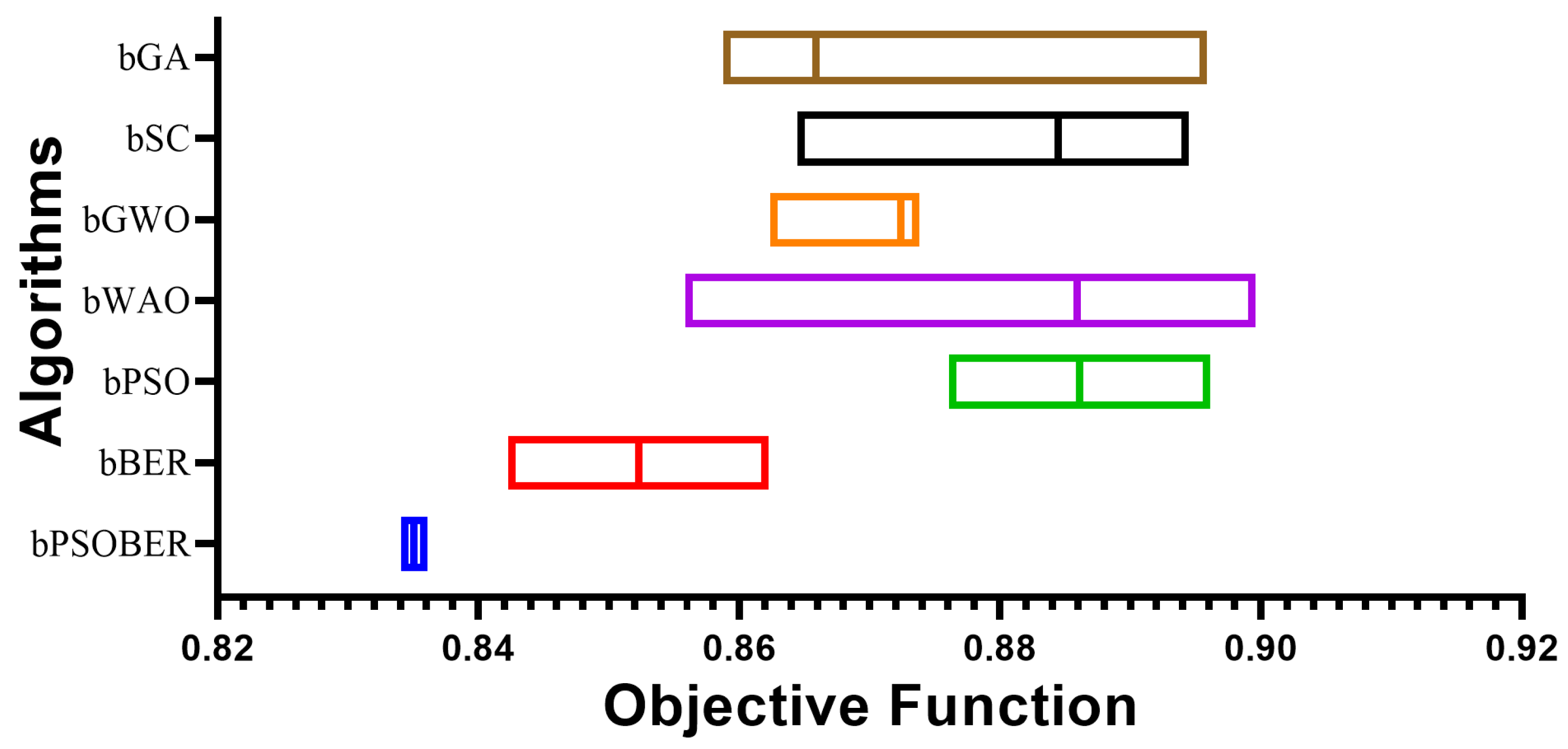
The results using the proposed feature selection method are illustrated by the plots shown in Figure 10. In this figure, the quartile–quartile (QQ), homoscedasticity, and residual plots are used to show the effectiveness and robustness of the proposed method. The values shown in the QQ plot approximately fit a straight line, which reflects the robustness of the selected features in classifying the monkepox cases. In addition, the recorded results in the homoscedasticity and residual plots give more emphasis to these findings.

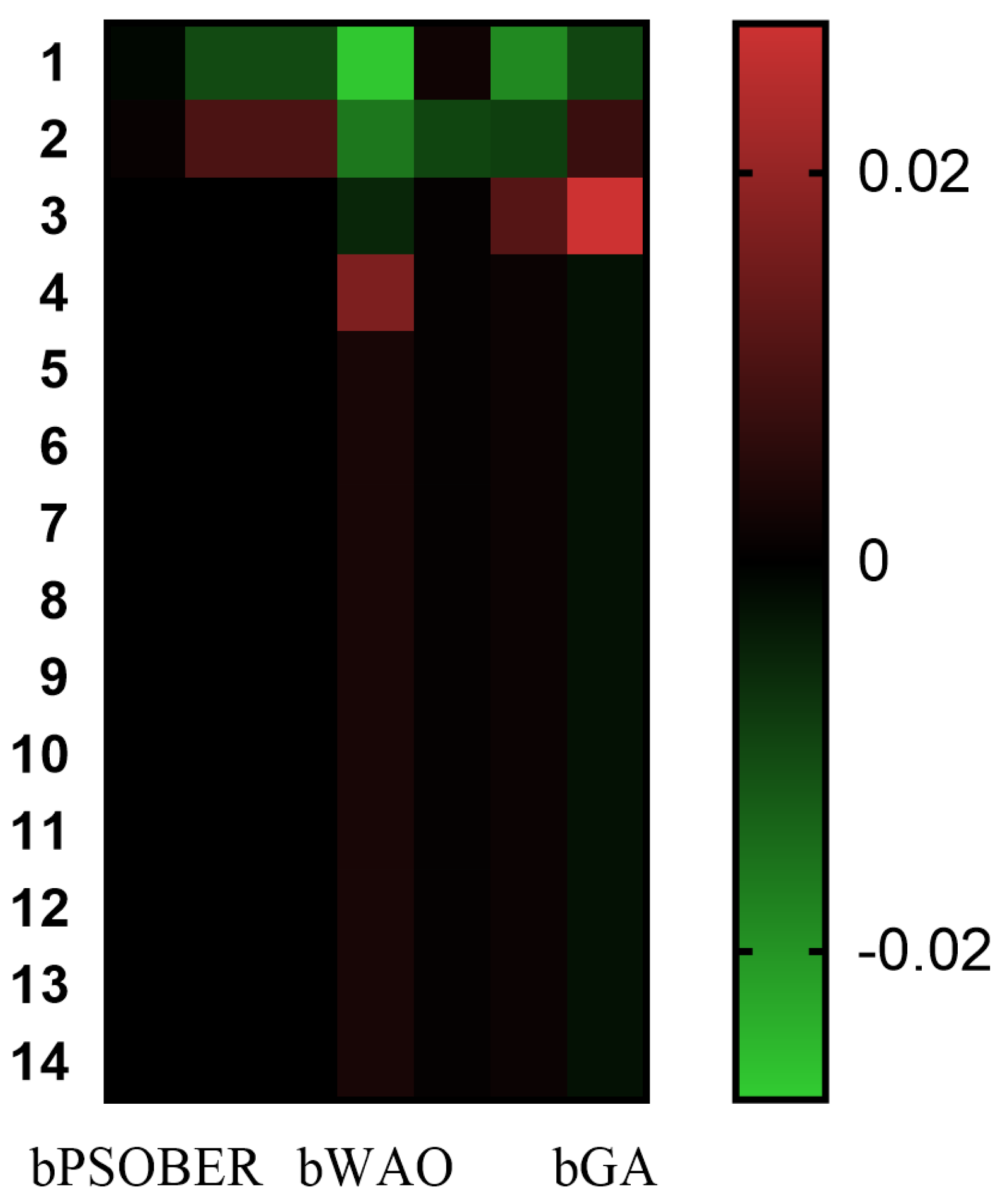
The average error of the proposed feature selection method compared to those of six other feature selection methods is shown in the plot depicted in Figure 11. In this figure, it is shown that the proposed method achieved the lowest average error, which confirms the robustness of the proposed method. In addition, the heatmap shown in Figure 12 confirms the superiority of bPSOBER, as it achieved the best results when compared to bWAO and bGA feature selection algorithms.

5.6. Stage 3: Monkeypox Classification Results

The selected features based on the proposed bPSOBER were used to classify the input image through a machine-learning classifier. The classifier adopted in this work was the multi-layer neural network (NN). To achieve the best performance of this NN, the parameters of this network were optimized using SCBER. The optimized parameters are listed in

Table 10. The optimized parameters of the developed neural network employed in monkeypox classification using SCBER.

Parameter	Optimized Value
Number of classes	2
Number of hidden layers	4
Neurons if the first layer	30
Number of neurons in the second layer	30
Number of neurons in the third layer	30
Number of neurons in the fourth layer	10
Training epochs	200
Learning rate	${10}^{-4}$
Display step	1
Batch size	100

.

The effectiveness of the optimized NN classifier was evaluated using a set of experiments. SCBER’s results are compared to those of BER, PSO, PSOBER, and SC to demonstrate the superiority of the proposed NN optimization. Various optimizers were employed to fine-tune the NN’s parameters, and the outcomes were recorded and analyzed.

Table 11. Statistical analysis of the results achieved by the optimized neural network using SCBER.

	SCBER+NN	BER+NN	PSO+NN	PSOBER+NN	SC+NN
Number of values	19	19	19	19	19
Minimum	0.989	0.9604	0.9625	0.9539	0.9539
10% Percentile	0.99	0.9704	0.9654	0.9594	0.9594
25% Percentile	0.99	0.9704	0.9654	0.9594	0.9594
75% Percentile	0.992	0.976	0.9754	0.9694	0.9694
90% Percentile	0.992	0.976	0.9754	0.9894	0.9694
95% CI of median
Maximum	0.992	0.976	0.9754	0.9994	0.9694
Median	0.99	0.9704	0.9654	0.9594	0.9594
Range	0.003	0.0156	0.0129	0.0455	0.0155
Actual confidence level	98.08%	98.08%	98.08%	98.08%	98.08%
Lower confidence limit	0.99	0.9704	0.9654	0.9594	0.9594
Upper confidence limit	0.992	0.976	0.9754	0.9694	0.9694
Mean	0.9906	0.9717	0.9684	0.9665	0.9623
Harmonic mean	0.9906	0.9717	0.9684	0.9663	0.9622
Quadratic mean	0.9906	0.9718	0.9684	0.9665	0.9623
Geometric mean	0.9906	0.9717	0.9684	0.9664	0.9623
Std. Error of Mean	0.0002334	0.000868	0.00113	0.002692	0.001177
Std. Deviation	0.001017	0.003783	0.004926	0.01173	0.005131
Upper 95% CI of mean	0.9911	0.9736	0.9708	0.9721	0.9647
Lower 95% CI of mean	0.9901	0.9699	0.966	0.9608	0.9598
Coefficient of variation	0.1027%	0.3893%	0.5087%	1.214%	0.5332%
Geometric SD factor	1.001	1.004	1.005	1.012	1.005
Upper 95% CI of geo. mean	0.9911	0.9736	0.9708	0.972	0.9647
Lower 95% CI of geo. mean	0.9901	0.9699	0.966	0.9608	0.9598
Upper 95% CI of harm. mean	0.9911	0.9736	0.9708	0.9719	0.9647
Lower 95% CI of harm. mean	0.9901	0.9699	0.966	0.9608	0.9598
Upper 95% CI of quad. mean	0.9911	0.9736	0.9708	0.9722	0.9648
Lower 95% CI of quad. mean	0.9901	0.9699	0.966	0.9608	0.9598
Kurtosis	−1.253	3.463	−1.391	2.688	−1.196
Skewness	0.6458	−1.177	0.7904	1.709	0.6007
Sum	18.82	18.46	18.4	18.36	18.28

presents a statistical analysis of the results achieved using SCBER compared to other optimization methods. Based on the results shown in this table, it is clear that the proposed optimization method yields superior results compared to the other methods.

The statistical significance of the proposed optimization of NN using SCBER was tested using the p-values by comparing the outputs of each pair of algorithms. The Wilcoxon’s rank-sum test was performed, and results were recorded. There are two major hypotheses at play here: the null and the alternative. The mean ($\mu$) values of null hypothesis represented by $H0$ include $\mu SCBER=\mu BER,\mu SCBER=\mu PSO,\mu SCBER=\mu PSOBER,\mu SCBER=\mu SC$. However, the $H1$ hypothesis does not factor in the averages of the algorithms. The outcomes of the Wilcoxon rank-sum test are shown in

Table 12. The Wilcoxon signed-rank test for evaluating the performance of the proposed optimization algorithm, SCBER, compared to other competing optimization methods.

	SCBER+NN	BER+NN	PSO+NN	PSOBER+NN	SC+NN
Theoretical median	0	0	0	0	0
Actual median	0.99	0.9704	0.9654	0.9594	0.9594
Number of values	19	19	19	19	19
Wilcoxon Signed Rank Test
Sum of signed ranks (W)	190	190	190	190	190
Sum of positive ranks	190	190	190	190	190
Sum of negative ranks	0	0	0	0	0
P value (two tailed)	<0.0001	<0.0001	<0.0001	<0.0001	<0.0001
Exact or estimate?	Exact	Exact	Exact	Exact	Exact
P value summary
Significant (alpha = 0.05)?	Yes	Yes	Yes	Yes	Yes
How big is the discrepancy?
Discrepancy	0.99	0.9704	0.9654	0.9594	0.9594

. Compared to the previous algorithms, the suggested one has a lower p-value (p < 0.005). The suggested feature selection approach was validated by these findings, demonstrating its statistical superiority. The ANOVA test was performed to examine whether or not there was a statistically significant difference between the suggested SCBER algorithm and the other algorithms. The mean ($\mu$) values of the null hypothesis, designated by $H0$, include $\mu SCBER=\mu BER$ = $\mu PSO=\mu PSOBER=\mu SC$. The measured values of the ANOVA test are presented in

Table 13. The results of the analysis of variance (ANOVA) test for evaluating the proposed SCBER+NN approach.

	SS	DF	MS	F (DFn, DFd)	p Value
Treatment (between columns)	0.009183	4	0.0023	F (4, 90) = 56.37	p < 0.0001
Residual (within columns)	0.003665	90	0.00004
Total	0.01285	94

. As presented in these tables, the results emphasize the superiority and effectiveness of the proposed approach in classifying monkeypox cases from images.

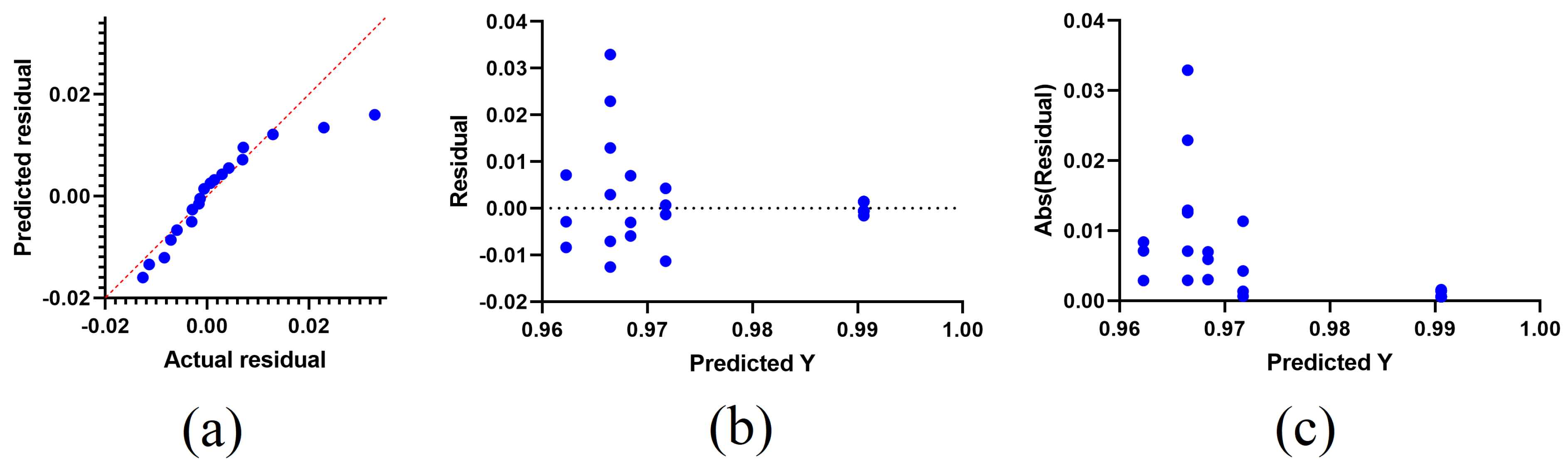
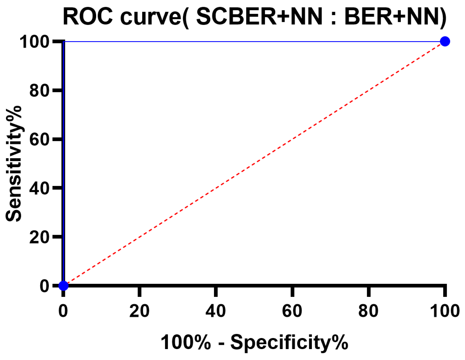
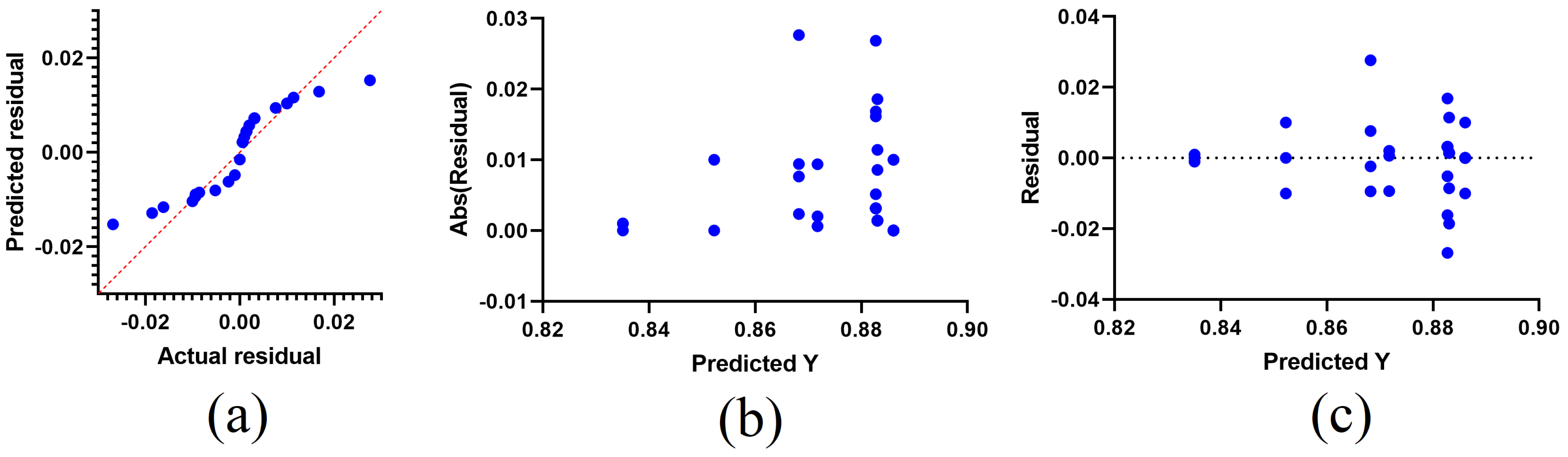
Figure 13 and Figure 14 graphically depict the statistical analysis of the achieved classification results. Figure 13 contains three plots, namely, a quartile–quartile (QQ) plot, a residual plot, and a homoscedasticity plot. Figure 14 illustrates the ROC curve. It can be seen in these graphs that SCBER is stable, with residual errors ranging from −0.02 to +0.02 and homoscedasticity values from −0.01 to +0.04. The QQ plot further demonstrates that the anticipated outcomes are consistent with the observed values, providing more evidence for the validity of the proposed method.

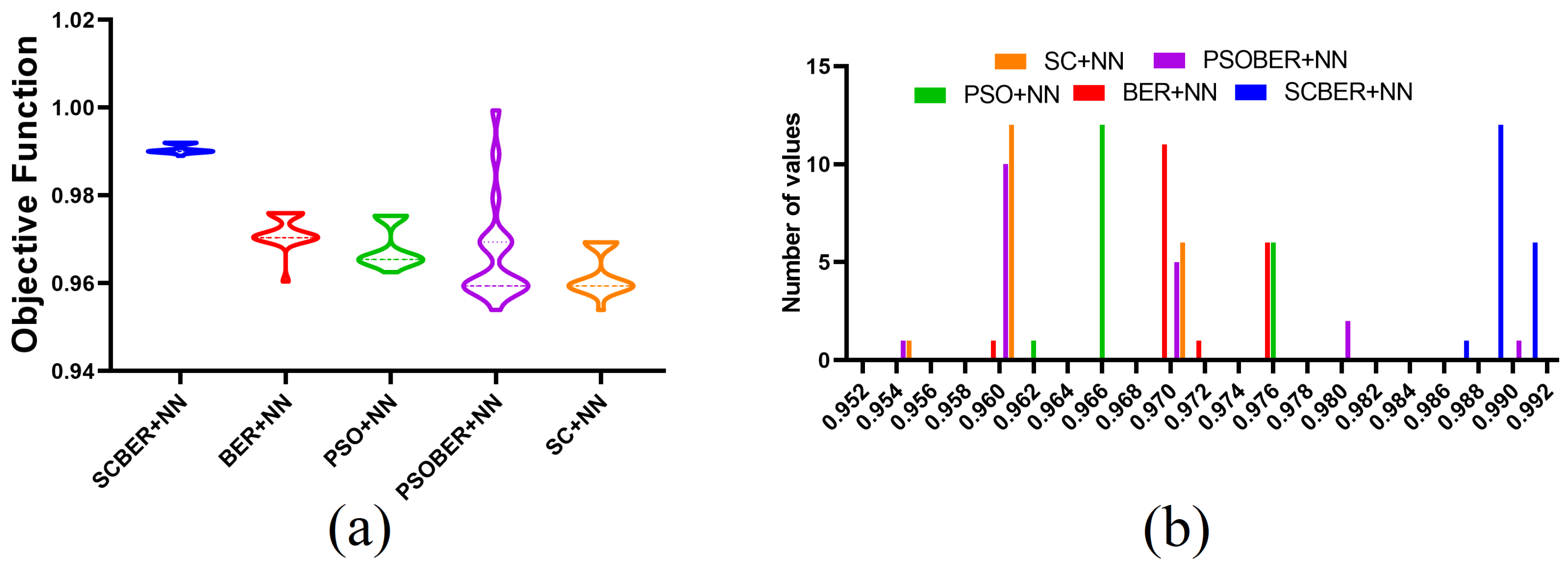
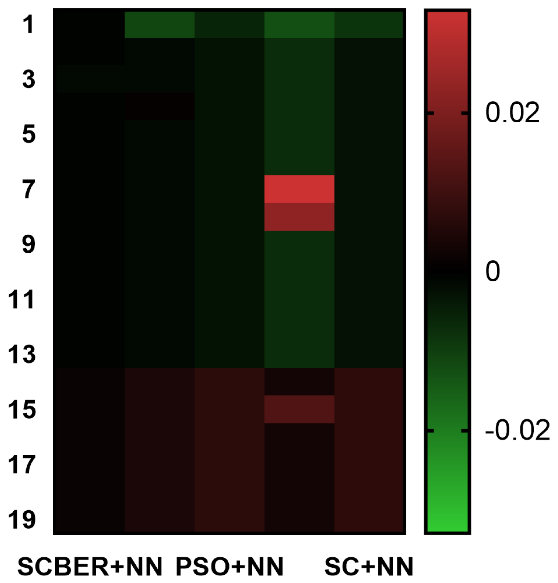
The accuracy plots depicted in Figure 15 and the heatmap plot depicted in Figure 16 show the accuracy and the histogram of the results achieved using SCBER. The accuracy plot shows that higher accuracy was achieved by the proposed algorithm compared to the other four optimization algorithm. In addition, the accuracy histogram plot emphasizes the superiority and stability of the proposed optimization algorithm in classifying the monkeypox cases in the input images.

6. Conclusions

In this paper, two algorithms were proposed for improving the classification accuracy of the monkeypox cases in images. The first algorithm is denoted the binary PSOBER algorithm, which is a hybrid of PSO and BER optimization algorithms and aims to select the best set of features that can improve the classification accuracy. The second algorithm is denoted by SCBER; it aims at optimizing the parameters of a NN to achieve the best accuracy. The evaluation of the proposed algorithms was performed with a freely-available monkeypox dataset which was augmented to fit the transfer learning using GoogleNet. Two sets of evaluation criteria were employed to assess the proposed algorithms. In addition, statistical analysis was performed by the Wilcoxon signed-rank test and ANOVA to measure the significance and effectiveness of the proposed algorithm. Moreover, a set of visual representations of the results was generated to confirm the robustness and effectiveness of the proposed algorithms. Experimental results show the superiority of the proposed algorithms compared to other competing algorithms in the task of monkeypox classification. The future aims of this work include assessing the proposed method with large-scale datasets and engineering optimization problems to clearly identify its advantages and disadvantages.

References

1. McCollum, A.M.; Damon, I.K. Human Monkeypox. Clin. Infect. Dis. 2014, 58, 260–267. [Google Scholar] [CrossRef] [Green Version]
2. Alakunle, E.; Moens, U.; Nchinda, G.; Okeke, M.I. Monkeypox Virus in Nigeria: Infection Biology, Epidemiology, and Evolution. Viruses 2020, 12, 1257. [Google Scholar] [CrossRef]
3. Moore, M.J.; Rathish, B.; Zahra, F. Monkeypox. In StatPearls; StatPearls Publishing: Treasure Island, FL, USA, 2022. [Google Scholar]
4. Nolen, L.D.; Osadebe, L.; Katomba, J.; Likofata, J.; Mukadi, D.; Monroe, B.; Doty, J.; Hughes, C.M.; Kabamba, J.; Malekani, J.; et al. Extended Human-to-Human Transmission during a Monkeypox Outbreak in the Democratic Republic of the Congo. Emerg. Infect. Dis. 2016, 22, 1014–1021. [Google Scholar] [CrossRef] [Green Version]
5. Nguyen, P.Y.; Ajisegiri, W.S.; Costantino, V.; Chughtai, A.A.; MacIntyre, C.R. Reemergence of Human Monkeypox and Declining Population Immunity in the Context of Urbanization, Nigeria, 2017–2020. Emerg. Infect. Dis. 2021, 27. [Google Scholar] [CrossRef]
6. El-kenawy, E.S.M.; Albalawi, F.; Ward, S.A.; Ghoneim, S.S.M.; Eid, M.M.; Abdelhamid, A.A.; Bailek, N.; Ibrahim, A. Feature Selection and Classification of Transformer Faults Based on Novel Meta-Heuristic Algorithm. Mathematics 2022, 10, 3144. [Google Scholar] [CrossRef]
7. Ali Salamai, A.; El-kenawy, E.S.M.; Abdelhameed, I. Dynamic Voting Classifier for Risk Identification in Supply Chain 4.0. Comput. Mater. Contin. 2021, 69, 3749–3766. [Google Scholar]
8. Ali, S.; Ahmed, M.; Paul, J.; Jahan, T.; Sani, S.; Noor, N.; Hasan, T. Monkeypox Skin Lesion Detection Using Deep Learning Models: A Feasibility Study. arXiv 2022, arXiv:2207.03342. [Google Scholar]
9. Adler, H.; Gould, S.; Hine, P.; Snell, L.B.; Wong, W.e.a. Clinical features and management of human monkeypox: A retrospective observational study in the UK. Lancet Infect. Dis. 2022, 22, 1153–1162. [Google Scholar] [CrossRef]
10. Akin, K.D.; Gurkan, C.; Budak, A.; KARATAŞ, H. Classification of Monkeypox Skin Lesion using the Explainable Artificial Intelligence Assisted Convolutional Neural Networks. Avrupa Bilim ve Teknoloji Dergisi 2022, 106–110. [Google Scholar] [CrossRef]
11. Ibrahim, A.; Mirjalili, S.; El-Said, M.; Ghoneim, S.S.M.; Al-Harthi, M.M.; Ibrahim, T.F.; El-Kenawy, E.S.M. Wind Speed Ensemble Forecasting Based on Deep Learning Using Adaptive Dynamic Optimization Algorithm. IEEE Access 2021, 9, 125787–125804. [Google Scholar] [CrossRef]
12. Ahsan, M.M.; Gupta, K.D.; Islam, M.M.; Sen, S.; Rahman, M.L.; Shakhawat Hossain, M. COVID-19 Symptoms Detection Based on NasNetMobile with Explainable AI Using Various Imaging Modalities. Mach. Learn. Knowl. Extr. 2020, 2, 490–504. [Google Scholar] [CrossRef]
13. Ahsan, M.M.; E. Alam, T.; Trafalis, T.; Huebner, P. Deep MLP-CNN Model Using Mixed-Data to Distinguish between COVID-19 and Non-COVID-19 Patients. Symmetry 2020, 12, 1526. [Google Scholar] [CrossRef]
14. Ahsan, M.M.; Ahad, M.T.; Soma, F.A.; Paul, S.; Chowdhury, A.; Luna, S.A.; Yazdan, M.M.S.; Rahman, A.; Siddique, Z.; Huebner, P. Detecting SARS-CoV-2 From Chest X-Ray Using Artificial Intelligence. IEEE Access 2021, 9, 35501–35513. [Google Scholar] [CrossRef]
15. Ahsan, M.M.; Nazim, R.; Siddique, Z.; Huebner, P. Detection of COVID-19 Patients from CT Scan and Chest X-ray Data Using Modified MobileNetV2 and LIME. Healthcare 2021, 9, 1099. [Google Scholar] [CrossRef]
16. Ahsan, M.M.; Siddique, Z. Machine learning-based heart disease diagnosis: A systematic literature review. Artif. Intell. Med. 2022, 128, 102289. [Google Scholar] [CrossRef]
17. Miranda, G.H.B.; Felipe, J.C. Computer-aided diagnosis system based on fuzzy logic for breast cancer categorization. Comput. Biol. Med. 2015, 64, 334–346. [Google Scholar] [CrossRef]
18. Ardakani, A.A.; Kanafi, A.R.; Acharya, U.R.; Khadem, N.; Mohammadi, A. Application of deep learning technique to manage COVID-19 in routine clinical practice using CT images: Results of 10 convolutional neural networks. Comput. Biol. Med. 2020, 121, 103795. [Google Scholar] [CrossRef]
19. Wang, L.; Lin, Z.Q.; Wong, A. COVID-Net: A tailored deep convolutional neural network design for detection of COVID-19 cases from chest X-ray images. Sci. Rep. 2020, 10, 19549. [Google Scholar] [CrossRef]
20. Sandeep, R.; Vishal, K.P.; Shamanth, M.S.; Chethan, K. Diagnosis of Visible Diseases Using CNNs. In Proceedings of the International Conference on Communication and Artificial Intelligence; Goyal, V., Gupta, M., Mirjalili, S., Trivedi, A., Eds.; Lecture Notes in Networks and Systems; Springer Nature: Singapore, 2022; pp. 459–468. [Google Scholar] [CrossRef]
21. Roy, K.; Chaudhuri, S.S.; Ghosh, S.; Dutta, S.K.; Chakraborty, P.; Sarkar, R. Skin Disease detection based on different Segmentation Techniques. In Proceedings of the 2019 International Conference on Opto-Electronics and Applied Optics (Optronix), Kolkata, India, 18–20 March 2019; pp. 1–5. [Google Scholar] [CrossRef]
22. Chandra, M.M.G. Effective Heart Disease Prediction Using Hybrid Machine Learning Techniques. Int. J. Sci. Res. Eng. Manag. 2022, 6. [Google Scholar] [CrossRef]
23. Wang, Z.; Zhu, X.; Adeli, E.; Zhu, Y.; Nie, F.; Munsell, B.; Wu, G. Multi-modal classification of neurodegenerative disease by progressive graph-based transductive learning. Med. Image Anal. 2017, 39, 218–230. [Google Scholar] [CrossRef] [PubMed]
24. Roman, R.C.; Precup, R.E.; Petriu, E.M. Hybrid data-driven fuzzy active disturbance rejection control for tower crane systems. Eur. J. Control 2021, 58, 373–387. [Google Scholar] [CrossRef]
25. Chi, R.; Li, H.; Shen, D.; Hou, Z.; Huang, B. Enhanced P-type Control: Indirect Adaptive Learning from Set-point Updates. IEEE Trans. Autom. Control. 2022. [Google Scholar] [CrossRef]
26. Wu, C.C.; Yeh, W.C.; Hsu, W.D.; Islam, M.M.; Nguyen, P.A.A.; Poly, T.N.; Wang, Y.C.; Yang, H.C.; Li (Jack), Y.C. Prediction of fatty liver disease using machine learning algorithms. Comput. Methods Programs Biomed. 2019, 170, 23–29. [Google Scholar] [CrossRef]
27. Qin, J.; Chen, L.; Liu, Y.; Liu, C.; Feng, C.; Chen, B. A Machine Learning Methodology for Diagnosing Chronic Kidney Disease. IEEE Access 2020, 8, 20991–21002. [Google Scholar] [CrossRef]
28. Khan, M.M.R.; Arif, R.B.; Siddique, M.A.B.; Oishe, M.R. Study and Observation of the Variation of Accuracies of KNN, SVM, LMNN, ENN Algorithms on Eleven Different Datasets from UCI Machine Learning Repository. In Proceedings of the 2018 4th International Conference on Electrical Engineering and Information & Communication Technology (iCEEiCT), Dhaka, Bangladesh, 13–15 September 2018; pp. 124–129. [Google Scholar] [CrossRef] [Green Version]
29. Abdar, M.; Książek, W.; Acharya, U.R.; Tan, R.S.; Makarenkov, V.; Pławiak, P. A new machine learning technique for an accurate diagnosis of coronary artery disease. Comput. Methods Programs Biomed. 2019, 179, 104992. [Google Scholar] [CrossRef]
30. Yu, Y.; Yang, Z.; Li, P.; Yang, Z.; You, Y. Work-in-Progress: On the Feasibility of Lightweight Scheme of Real-Time Atrial Fibrillation Detection Using Deep Learning. In Proceedings of the 2019 IEEE Real-Time Systems Symposium (RTSS), Hong Kong, 3–6 December 2019; pp. 552–555. [Google Scholar] [CrossRef]
31. Hayward, G. Remarks on Smallpox, Cowpox and Varioloid. Boston Med. Surg. J. 1860, 62, 173–177. [Google Scholar] [CrossRef]
32. Islam, T.; Hussain, M.A.; Chowdhury, F.U.H.; Islam, B.M.R. A Web-scraped Skin Image Database of Monkeypox, Chickenpox, Smallpox, Cowpox, and Measles. bioRxiv 2022. [Google Scholar] [CrossRef]
33. Chen, J.; Wu, L.; Zhang, J.; Zhang, L.; Gong, D.; Zhao, Y.; Chen, Q.; Huang, S.; Yang, M.; Yang, X.; et al. Deep learning-based model for detecting 2019 novel coronavirus pneumonia on high-resolution computed tomography. Sci. Rep. 2020, 10, 19196. [Google Scholar] [CrossRef]
34. El-Kenawy, E.S.M.; Mirjalili, S.; Alassery, F.; Zhang, Y.D.; Eid, M.M.; El-Mashad, S.Y.; Aloyaydi, B.A.; Ibrahim, A.; Abdelhamid, A.A. Novel Meta-Heuristic Algorithm for Feature Selection, Unconstrained Functions and Engineering Problems. IEEE Access 2022, 10, 40536–40555. [Google Scholar] [CrossRef]
35. Abdelhamid, A.A.; El-Kenawy, E.S.M.; Alotaibi, B.; Amer, G.M.; Abdelkader, M.Y.; Ibrahim, A.; Eid, M.M. Robust Speech Emotion Recognition Using CNN+LSTM Based on Stochastic Fractal Search Optimization Algorithm. IEEE Access 2022, 10, 49265–49284. [Google Scholar] [CrossRef]
36. Han, J.; Zhang, D.; Cheng, G.; Liu, N.; Xu, D. Advanced Deep-Learning Techniques for Salient and Category-Specific Object Detection: A Survey. IEEE Signal Process. Mag. 2018, 35, 84–100. [Google Scholar] [CrossRef]
37. Simonyan, K.; Zisserman, A. Very Deep Convolutional Networks for Large-Scale Image Recognition. In Proceedings of the International Conference on Learning Representations, San Diego, CA, USA, 7–9 May 2015; pp. 1–14. [Google Scholar]
38. Yu, S.; Xie, L.; Liu, L.; Xia, D. Learning Long-Term Temporal Features with Deep Neural Networks for Human Action Recognition. IEEE Access 2020, 8, 1840–1850. [Google Scholar] [CrossRef]
39. Al-Dhamari, A.; Sudirman, R.; Mahmood, N.H. Transfer Deep Learning Along with Binary Support Vector Machine for Abnormal Behavior Detection. IEEE Access 2020, 8, 61085–61095. [Google Scholar] [CrossRef]
40. Atkinson, P.M.; Tatnall, A.R.L. Introduction Neural networks in remote sensing. Int. J. Remote Sens. 1997, 18, 699–709. [Google Scholar] [CrossRef]
41. Patra, S.; Ghosh, S.; Ghosh, A. Histogram thresholding for unsupervised change detection of remote sensing images. Int. J. Remote Sens. 2011, 32, 6071–6089. [Google Scholar] [CrossRef]
42. Khafaga, D.S.; Alhussan, A.A.; El-Kenawy, E.S.M.; Ibrahim, A.; Eid, M.M.; Abdelhamid, A.A. Solving Optimization Problems of Metamaterial and Double T-Shape Antennas Using Advanced Meta-Heuristics Algorithms. IEEE Access 2022, 10, 74449–74471. [Google Scholar] [CrossRef]
43. Alhussan, A.A.; Khafaga, D.S.; El-Kenawy, E.S.M.; Ibrahim, A.; Eid, M.M.; Abdelhamid, A.A. Pothole and Plain Road Classification Using Adaptive Mutation Dipper Throated Optimization and Transfer Learning for Self Driving Cars. IEEE Access 2022, 10, 84188–84211. [Google Scholar] [CrossRef]
44. Mirjalili, S. SCA: A Sine Cosine Algorithm for solving optimization problems. Knowl.-Based Syst. 2016, 96, 120–133. [Google Scholar] [CrossRef]
45. Eid, M.M.; El-kenawy, E.S.M.; Ibrahim, A. A Binary Sine Cosine-Modified Whale Optimization Algorithm for Feature Selection. In Proceedings of the National Computing Colleges Conference (NCCC), Taif, Saudi Arabia, 27–28 March 2021; pp. 1–6. [Google Scholar] [CrossRef]
46. Bala, D. Monkeypox Skin Images Dataset (MSID). 2022. Available online: https://www.kaggle.com/datasets/dipuiucse/monkeypoxskinimagedataset?resource=download (accessed on 10 September 2022).
47. El-Kenawy, E.S.M.; Mirjalili, S.; Abdelhamid, A.A.; Ibrahim, A.; Khodadadi, N.; Eid, M.M. Meta-Heuristic Optimization and Keystroke Dynamics for Authentication of Smartphone Users. Mathematics 2022, 10, 2912. [Google Scholar] [CrossRef]
48. Bello, R.; Gomez, Y.; Nowe, A.; Garcia, M.M. Two-Step Particle Swarm Optimization to Solve the Feature Selection Problem. In Proceedings of the Seventh International Conference on Intelligent Systems Design and Applications (ISDA 2007), Rio de Janeiro, Brazil, 22–24 October 2007; pp. 691–696. [Google Scholar] [CrossRef]
49. Mirjalili, S.; Lewis, A. The Whale Optimization Algorithm. Adv. Eng. Softw. 2016, 95, 51–67. [Google Scholar] [CrossRef]
50. El-kenawy, E.S.; Eid, M. Hybrid Gray Wolf and Particle Swarm Optimization for Feature Selection. Int. J. Innov. Comput. Inf. Control. IJICIC 2020, 16, 831–844. [Google Scholar] [CrossRef]
51. Fister, I.; Yang, X.-S.; Fister, I.; Brest, J. Memetic firefly algorithm for combinatorial optimization. In Bioinspired Optimization Methods and Their Applications—(BIOMA 2012); Filipic, B., Silc, J., Eds.; Jozef Stefan Institute: Ljubljana, Slovenia, 2012; pp. 75–86. [Google Scholar]
52. Kabir, M.M.; Shahjahan, M.; Murase, K. A new local search based hybrid genetic algorithm for feature selection. Neurocomputing 2011, 74, 2914–2928. [Google Scholar] [CrossRef]
Figure 1. Architecture of GoogleNet, the deep network employed for feature extraction based on transfer learning.
Mathematics 10 03614 g001
Figure 2. Architecture of the neural network employed for monkeypox classification.
Mathematics 10 03614 g002
Figure 3. The measurement of Earth’s radius using the Al-Biruni method.
Mathematics 10 03614 g003
Figure 4. The process of the sine cosine optimization algorithm.
Mathematics 10 03614 g004
Figure 5. Particle swarm optimization.
Mathematics 10 03614 g005
Figure 6. The stages of the proposed monkeypox classification methodology.
Mathematics 10 03614 g006
Figure 7. Sample set of images from the monkeypox dataset.
Mathematics 10 03614 g007
Figure 8. The countries contaminated with the monkeypox virus.
Mathematics 10 03614 g008
Figure 9. The operations of data augmentation applied to the monkeypox dataset. Data augmentation was used for the training and validation sets only.
Mathematics 10 03614 g009
Figure 10. Analysis plots of the achieved results based on the proposed feature selection algorithm, bPSOBER. (a) QQ plot, (b) Homoscedasticity plot, (c) Residual plot.
Mathematics 10 03614 g010
Figure 11. The average error of the results achieved based on the proposed feature selection algorithm, bPSOBER.
Mathematics 10 03614 g011
Figure 12. Heatmap of the achieved results based on the proposed feature selection algorithm, bPSOBER.
Mathematics 10 03614 g012
Figure 13. Analysis plots of the achieved classification results based on a neural network optimized using the proposed SCBER algorithm. (a) QQ plot, (b) Homoscedasticity plot, (c) Residual plot.
Mathematics 10 03614 g013
Figure 14. The ROC curve of the results achieved by the neural network optimized using SCBER in comparison with the results achieved by the neural network optimized using BER.
Mathematics 10 03614 g014
Figure 15. The accuracy plot and accuracy histogram plot of the results achieved by the proposed SCBER algorithm, and four other optimization algorithms. (a) Accuracy plot. (b) Histogram plot.
Mathematics 10 03614 g015
Figure 16. The heatmap of the results achieved by the neural network optimized using the proposed SCBER algorithm compared to the other competing algorithms.
Mathematics 10 03614 g016