A Fitted Operator Finite Difference Approximation for Singularly Perturbed Volterra–Fredholm Integro-Differential Equations

Abstract

This paper presents a ε-uniform and reliable numerical scheme to solve second-order singularly perturbed Volterra–Fredholm integro-differential equations. Some properties of the analytical solution are given, and the finite difference scheme is established on a non-uniform mesh by using interpolating quadrature rules and the linear basis functions. An error analysis is successfully carried out on the Boglaev–Bakhvalov-type mesh. Some numerical experiments are included to authenticate the theoretical findings. In this regard, the main advantage of the suggested method is to yield stable results on layer-adapted meshes.

1. Introduction

Volterra–Fredholm integro-differential equations (VFIDEs) have led to many scientific computings. They play important roles in different branches of science involving aerodynamics, the economy, electricity and electronics, industrial networks, hydrodynamics, oceanography and chemistry [1,2,3] (see the references detailed within). Particularly, VFIDEs have been used widely for population growth, medicine processes and pandemic research. For example, the dissipation of tumor cells and the response of immune system were modeled in [4]. The effect of the COVID-19 pandemic was investigated in Italy, Germany and France with the help of modeling by some integro-differential equations [5,6].

Some existence and uniqueness results for VFIDEs have been presented by Hamoud and his co-authors in [7,8]. Due to their importance in computational science, numerous methods have been introduced for solving VFIDEs. Various semi-analytical techniques including Adomian decomposition method, variational iteration method, homotopy perturbation method, modified differential transform method and Laplace decomposition method have been proposed in [2,9,10]. Furthermore, many scholars have developed different numerical approaches. These include the exponential spline method [11], the collocation method [1], the Nyström method [12], reproducing the kernel method [13], the Haar wavelet [14,15], the Chebyshev–Galerkin method [16], the operational matrix method of Bernstein polynomials [17], the finite difference method [18,19], the Galerkin method [20,21], the bezier curve method [22], etc. [3,23,24,25,26]. The mentioned studies have only dealt with regular cases (i.e., absent the singularity).

This article concerns with boundary-value problem of second-order Volterra–Fredholm integro-differential equation in the form

$$Lu+Tu+Su=f\left(x\right),x\in \overline{I},$$

(1)

subject to boundary conditions

$$u\left(0\right)=A,u\left(l\right)=B,$$

(2)

in which the differential operator $Lu$, the Volterra integral operator T and the Fredholm integral operator S are given as follow, respectively:

$$Lu=-{\epsilon }^2{u}^{″}+a\left(x\right)u,Tu=\lambda \underset{0}{\overset{x}{\int }}{K}_1(x,t)u\left(t\right)dt$$

and

$$Su=\lambda \underset{0}{\overset{l}{\int }}{K}_2(x,t)u\left(t\right)dt.$$

Additionally, $\epsilon \in \left(0,1\right]$ is a small parameter, $\overline{I}=[0,l],$$\lambda$ is a real parameter, the functions $a\left(x\right)\ge \alpha >0,$ $f\left(x\right)$$\left(x\in \overline{I}\right),u\left(x\right)$$\left(x\in \overline{I}\right),$$K_1(x,t)$ and $K_2(x,t)$$\left(\left(x,t\right)\in \overline{I}\times \overline{I}\right)$ are sufficiently smooth. Under these conditions, the problem (1) and (2) has unique solution $u$. As $\epsilon$ tends toward zero, the boundary layers appear in neighborhood of $x=0$ and $x=l$.

In recent times, a lot of papers have been published about singularly perturbed integro-differential equations and various numerical schemes have been suggested. Iragi and Munyakazi have considered fitted operator finite difference method by using right-side rectangle rule and trapezoidal integration on Shishkin mesh for Volterra integro-differential equations with singularity [27,28]. In [29,30,31], Volterra delay integro-differential equations with initial layer have been investigated on uniform mesh. Mbroh et. al. have proposed non-standard finite difference scheme by using composite Simpson’s rule. Additionally, they have improved the order of convergence by applying Richardson extrapolation [32]. In [33], second-order discretization have been presented on piecewise uniform mesh. Tao and Zhang have introduced the coupled method involving local discontinuous Galerkin technique and continuous finite element method in [34]. In [35], using composite trapezoidal rule, fitted mesh finite difference schemes have been established on Shishkin type mesh. Moreover, almost second-order accuracies for the presented method have been obtained. Exponentially fitted difference schemes have been suggested for singularly perturbed Fredholm integro-differential equations in [36,37,38]. In [39], Durmaz and Amiraliyev have constructed fitted second-order homogeneous difference scheme on Shishkin mesh for Fredholm integro differential equations with layer behavior. Authors in [40,41] have presented a new discrete scheme for singularly perturbed Volterra-Fredholm integro-differential equations.

To the best of our knowledge, the problems in (1) and (2) have not been investigated using the finite difference schemes. Therefore, this study aims to fill this gap. This paper introduces the new difference scheme for the boundary value problems of second-order singularly perturbed Volterra–Fredholm integro-differential equations as the major novelty of this work. The second contribution is the convergence analysis of the presented scheme on Boglaev–Bakhvalov-type mesh. Last but not least, the proposed algorithm is easy to construct, and it provides stable results in a short time in terms of computation. From these objectives, the theory and applications of the presented method have been extensively studied.

The remainder of this article is organized is as follows. In Section 2, first, some preliminary results are given. Then, using composite numerical quadrature rules and implicit difference rules, the finite difference scheme is constructed on Boglaev–Bakhvalov-type mesh in Section 3. Section 4 is devoted to error approximations and stability analysis. In Section 5, three numerical examples are solved by the proposed method. Furthermore, the corresponding algorithm and the computational results are presented. Finally, the paper ends with “Concluding Remarks”.

2. Asymptotic Properties

This section is devoted to some a priori bounds. For this aim, the following lemma is expressed.

Lemma 1.

We assume that $a,f\in C^1\left[0,l\right]$, $\frac{{\partial }^s{K}_1}{\partial x^s}\in C{\left[0,l\right]}^2,\frac{{\partial }^s{K}_2}{\partial x^s}\in C{\left[0,l\right]}^2,(s=0,1)$, ${\overline{K}}_1={\displaystyle \underset{\overline{I}\times \overline{I}}{max}}\left|K_1(x,t)\right|$, ${\overline{K}}_2={\displaystyle \underset{\overline{I}\times \overline{I}}{max}}\left|K_2(x,t)\right|$ and

$$\left|\lambda \right|<\frac{\alpha }{{\displaystyle \underset{0\le x\le l}{max}}\underset{0}{\overset{x}{\int }}\left|K_1(x,t)\right|dt+{\displaystyle \underset{0\le x\le l}{max}}\underset{0}{\overset{l}{\int }}\left|K_2(x,t)\right|dt}.$$

(3)

Then, the solution $u\left(x\right)$ of the problems in (1) and (2) holds

$${∥u∥}_{\infty }\le C_0$$

(4)

and

$$\left|u^{\prime }\left(x\right)\right|\le C\left\{1+\frac{1}{\epsilon }\left(e^{\frac{-\sqrt{\alpha }x}{\epsilon }}+e^{\frac{-\sqrt{\alpha }(l-x)}{\epsilon }}\right)\right\},0<x<l,$$

(5)

where

$$C_0={\left(1-\gamma \right)}^{-1}\left(\left|A\right|+\left|B\right|+{\alpha }^{-1}{∥f∥}_{\infty }\right)$$

and

$$\gamma ={\alpha }^{-1}\left|\lambda \right|{\displaystyle \underset{0\le x\le l}{max}}\stackrel{x}{\underset{0}{\int }}\left|K_1(x,t)\right|dt+{\alpha }^{-1}\left|\lambda \right|{\displaystyle \underset{0\le x\le l}{max}}\stackrel{l}{\underset{0}{\int }}\left|K_2(x,t)\right|dt<1.$$

Proof. 

By considering the maximum principle for the problems in (1)–(2), we obtain

$$\begin{array}{ccc}\hfill \left|u\left(x\right)\right|& \le & \left|A\right|+\left|B\right|+{\alpha }^{-1}{\displaystyle \underset{0\le x\le l}{max}}\left|f\left(x\right)\right|+{\alpha }^{-1}\left|\lambda \right|{\displaystyle \underset{0\le x\le l}{max}}\underset{0}{\overset{x}{\int }}\left|K_1(x,t)\right|\left|u\left(t\right)\right|dt\hfill \\ & & +{\alpha }^{-1}\left|\lambda \right|{\displaystyle \underset{0\le x\le l}{max}}\underset{0}{\overset{l}{\int }}\left|K_2(x,t)\right|\left|u\left(t\right)\right|dt.\hfill \end{array}$$

Then, it follows that

$${∥u∥}_{\infty }\le \left|A\right|+\left|B\right|+{\alpha }^{-1}{∥f∥}_{\infty }+{\alpha }^{-1}\left|\lambda \right|{\displaystyle \underset{0\le x\le l}{max}}\underset{0}{\overset{x}{\int }}\left|K_1(x,t)\right|dt{∥u∥}_{\infty }$$

$$+{\alpha }^{-1}\left|\lambda \right|{\displaystyle \underset{0\le x\le l}{max}}\underset{0}{\overset{l}{\int }}\left|K_2(x,t)\right|dt{∥u∥}_{\infty }.$$

Finally, we have

$${∥u∥}_{\infty }\le {\left(1-\gamma \right)}^{-1}\left(\left|A\right|+\left|B\right|+{\alpha }^{-1}{∥f∥}_{\infty }\right).$$

By taking into consideration (3), we reach the proof of the (4). Now, we prove the relation (5). Since $\left|K_1\right|\le {\overline{K}}_1$, $\left|K_2\right|\le {\overline{K}}_2$ and $\left|u\left(x\right)\right|\le C$, we can write for the second derivative of $u\left(x\right)$

$$\left|u^{″}\left(x\right)\right|\le \frac{1}{{\epsilon }^2}\left[\left|f\left(x\right)\right|+\left|a\left(x\right)\right|\left|u\left(x\right)\right|\right.$$

$$\left.+\left|\lambda \right|\underset{0}{\overset{x}{\int }}\left|K_1(x,t)\right|\left|u\left(t\right)\right|dt+\left|\lambda \right|\underset{0}{\overset{l}{\int }}\left|K_2(x,t)\right|\left|u\left(t\right)\right|dt\right]\le \frac{C}{{\epsilon }^2},0\le x\le l.$$

For any function $g\in C^2\left[0,l\right]$, the following formula is used to estimate $\left|u^{\prime }\left(0\right)\right|$ and $\left|u^{\prime }\left(l\right)\right|:$

$$g^{\prime }\left(x\right)=g\left[{\alpha }_0,{\alpha }_1\right]-\underset{{\alpha }_0}{\overset{{\alpha }_1}{\int }}{K}_0(\xi ,x)g^{″}\left(\xi \right)d\xi ,{\alpha }_0<{\alpha }_1,$$

(6)

where

$$g\left[{\alpha }_0,{\alpha }_1\right]=\frac{g\left({\alpha }_1\right)-g\left({\alpha }_0\right)}{{\alpha }_1-{\alpha }_0},$$

$$K_0(\xi ,x)=T_0(\xi -x)-{\left({\alpha }_1-{\alpha }_0\right)}^{-1}(\xi -{\alpha }_0)$$

and

$$T_0\left(\lambda \right)=\left\{\begin{array}{c}1,\lambda \ge 0,\\ 0,\lambda <0.\end{array}\right.$$

In (6), by taking $g\left(x\right)=u\left(x\right),x=0,{\alpha }_0=0$ and ${\alpha }_1=\epsilon$, we find the estimation of $\left|u^{\prime }\left(0\right)\right|:$

$$\left|u^{\prime }\left(0\right)\right|\le \frac{u\left(\epsilon \right)-u\left(0\right)}{\epsilon }-\underset{0}{\overset{\epsilon }{\int }}{K}_0(\xi ,0)u^{″}\left(\xi \right)d\xi \le \frac{C}{\epsilon }.$$

In the same way, rewriting $g\left(x\right)=u\left(x\right),x=l,{\alpha }_0=l-\epsilon$ and ${\alpha }_1=l$ in (6), we obtain

$$\left|u^{\prime }\left(l\right)\right|\le \frac{u\left(l\right)-u\left(\epsilon \right)}{\epsilon }-\underset{l-\epsilon }{\overset{l}{\int }}{K}_0(\xi ,l)u^{″}\left(\xi \right)d\xi \le \frac{C}{\epsilon }.$$

Differentiating (1), we have

$$-{\epsilon }^2{v}^{″}+a\left(x\right)v=F\left(x\right),$$

(7)

$$v\left(0\right)=O\left(\frac{1}{\epsilon }\right),v\left(l\right)=O\left(\frac{1}{\epsilon }\right).$$

(8)

From (4), it is clear that

$$\left|F\left(x\right)\right|\le C.$$

(9)

We investigate the solution of the problems in (7) and (8) in the following form:

$$v\left(x\right)=v_1\left(x\right)+v_2\left(x\right),$$

Here, the functions $v_1\left(x\right)$ and $v_2\left(x\right)$ are the solutions of the following problems, respectively:

$$-{\epsilon }^2{v}_1^{″}+a\left(x\right)v_1=F\left(x\right),$$

(10)

$$v_1\left(0\right)=v_1\left(l\right)=0$$

(11)

and

$$-{\epsilon }^2{v}_2^{″}+a\left(x\right)v_2=0,$$

(12)

$$v_2\left(0\right)=O\left(\frac{1}{\epsilon }\right),v_2\left(l\right)=O\left(\frac{1}{\epsilon }\right).$$

(13)

By using the maximum principle, we obtain

$$\left|v_1\left(x\right)\right|\le {\alpha }^{-1}{∥F∥}_{\infty }\le C,0\le x\le l,$$

(14)

and

$$\left|v_2\left(x\right)\right|\le w\left(x\right).$$

(15)

Here, the function $w\left(x\right)$ is the solution of the following problem:

$$-{\epsilon }^2{w}^{″}\left(x\right)+aw=0,$$

(16)

$$w\left(0\right)=\left|v_2\left(0\right)\right|,w\left(l\right)=\left|v_2\left(l\right)\right|.$$

(17)

For the solution of the problems in (16) and (17), it is obvious that

$$w\left(x\right)=\frac{1}{sinh\left(\frac{\sqrt{\alpha }l}{\epsilon }\right)}\left\{w\left(0\right)sinh\left(\frac{\sqrt{\alpha }(l-x)}{\epsilon }\right)+w\left(l\right)sinh\left(\frac{\sqrt{\alpha }l}{\epsilon }\right)\right\}.$$

From here, we can write

$$w\left(x\right)\le \frac{C}{\epsilon }\left\{e^{\frac{-\sqrt{\alpha }x}{\epsilon }}+e^{\frac{-\sqrt{\alpha }(l-x)}{\epsilon }}\right\}.$$

(18)

Thus, we obtain

$$\left|u^{\prime }\left(x\right)\right|\le \left|v_1\left(x\right)\right|+\left|v_2\left(x\right)\right|,$$

which hints at the proof of the relation (5) [42]. Therefore, the proof of the lemma is completed.   □

3. Discrete Scheme

In this section, the finite difference discretization is presented for the problem (1) and (2). First, we give the definition of the mesh. Let ${\omega }_N$ be a non-uniform mesh on $\left[0,l\right]$:

$${\omega }_N=\left\{0<x_1<x_2<\dots <x_{N-1,}{h}_i=x_i-x_{i-1}\right\}$$

and

$${\overline{\omega }}_N={\omega }_N\cup \left\{x_0=0,x_N=l\right\}.$$

Here, we use the non-uniform mesh called Boglaev–Bakhvalov-type mesh in  [43]. The transition point is taken as

$${\sigma }_1=min\{\frac{l}{4},{\alpha }^{-1}\epsilon \left|ln\epsilon \right|\}.$$

For an even number N, we divide each of the subintervals $\left[0,{\sigma }_1\right],\left[{\sigma }_1,{\sigma }_2\right]$ and $\left[{\sigma }_2,l\right]$. Here, ${\sigma }_2=l-{\sigma }_1$. $x_i$ node points are specified as

$$x_i=\left\{\begin{array}{c}-{\alpha }^{-1}\epsilon ln\left(1-(1-\epsilon )\frac{4i}{N}\right),i=0,1,\dots ,\frac{N}{4},x_i\in \left[0,{\sigma }_1\right],{\sigma }_1<\frac{l}{4};\\ -{\alpha }^{-1}\epsilon ln\left(1-(1-e^{-\frac{\alpha l}{4\epsilon }})\frac{4i}{N}\right),i=0,1,\dots ,\frac{N}{4},x_i\in \left[0,{\sigma }_1\right],{\sigma }_1=\frac{l}{4};\\ {\sigma }_1+(i-\frac{N}{4})h^{\left(1\right)},i=\frac{N}{4}+1,\dots ,\frac{3N}{4},x_i\in \left[{\sigma }_1,{\sigma }_2\right],h^{\left(1\right)}=\frac{2({\sigma }_2-{\sigma }_1)}{N};\\ {\sigma }_2-{\alpha }^{-1}\epsilon ln\left(1-(1-\epsilon )\frac{4\left(i-\frac{3N}{4}\right)}{N}\right),i=\frac{3N}{4}+1,\dots ,N,x_i\in \left[{\sigma }_2,l\right],{\sigma }_2<\frac{3l}{4};\\ {\sigma }_2-{\alpha }^{-1}\epsilon ln\left(1-(1-e^{-\frac{\alpha l}{4\epsilon }})\frac{4\left(i-\frac{3N}{4}\right)}{N}\right),i=\frac{3N}{4}+1,\dots ,N,x_i\in \left[{\sigma }_2,l\right],{\sigma }_2=\frac{3l}{4}.\end{array}\right.$$

Before constructing the difference scheme, we define some notation for the mesh functions. For any mesh function $v\left(x\right)$ defined on ${\overline{\omega }}_N$, we use the following implicit difference rules:

$$v_i=v\left(x_i\right),v_{\overline{x},i}=\frac{v_i-v_{i-1}}{h_i},$$

$$v_{x,i}=\frac{v_{i+1}-v_i}{h_{i+1}},v_{\overline{x}\widehat{x},i}=\frac{1}{{\hslash }_i}\left(v_{x,i}-v_{\overline{x},i}\right).$$

Here, ${\hslash }_i$ is defined as

$${\hslash }_i=\frac{1}{2}\left(h_i+h_{i+1}\right)$$

and the discrete maximum norm is denoted by

$${∥v∥}_{\infty }={∥v∥}_{\infty ,{\overline{\omega }}_N}={\displaystyle \underset{0\le i\le N}{max}}\left|v_i\right|.$$

To establish the difference scheme for the problems in (1) and (2), we use the following integral identity:

$${\hslash }_i^{-1}\underset{x_{i-1}}{\overset{x_{i+1}}{\int }}\left[Lu+Tu+Su\right]{\phi }_i\left(x\right)dx={\hslash }_i^{-1}\underset{x_{i-1}}{\overset{x_{i+1}}{\int }}f\left(x\right){\phi }_i\left(x\right)dx,i=1,2,\dots ,N-1,$$

(19)

where the basis function is defined as follows:

$${\phi }_i\left(x\right)=\left\{\begin{array}{cc}{\phi }_i^{\left(1\right)}\left(x\right)=\frac{x-x_{i-1}}{h_i},\hfill & x\in (x_{i-1},x_i)\hfill \\ {\phi }_i^{\left(2\right)}\left(x\right)=\frac{x_{i+1}-x}{h_{i+1}},\hfill & x\in (x_i,x_{i+1})\hfill \\ 0,\hfill & x\notin (x_{i-1},x_{i+1}).\hfill \end{array}\right.$$

Moreover, it can be easily seen that

$${\hslash }_i^{-1}\underset{x_{i-1}}{\overset{x_{i+1}}{\int }}{\phi }_i\left(x\right)dx={\hslash }_i^{-1}\left(\frac{h_i}{2}+\frac{h_{i+1}}{2}\right)=1.$$

For the differential operator $Lu$ in (19), after using interpolating quadrature rules in [44] and some manipulations, we find

$${\hslash }_i^{-1}\underset{x_{i-1}}{\overset{x_{i+1}}{\int }}Lu{\phi }_i\left(x\right)dx={\hslash }_i^{-1}{\epsilon }^2\underset{x_{i-1}}{\overset{x_i}{\int }}{u}^{\prime }{\phi }_i^{{\left(1\right)}^{{}^{\prime }}}\left(x\right)dx+{\hslash }_i^{-1}{\epsilon }^2\underset{x_i}{\overset{x_{i+1}}{\int }}{u}^{\prime }{\phi }_i^{{\left(2\right)}^{{}^{\prime }}}\left(x\right)dx$$

$$+a_i{\hslash }_i^{-1}\underset{x_{i-1}}{\overset{x_i}{\int }}u\left(x\right){\phi }_i^{\left(1\right)}\left(x\right)dx+a_i{\hslash }_i^{-1}\underset{x_i}{\overset{x_{i+1}}{\int }}u\left(x\right){\phi }_i^{\left(2\right)}\left(x\right)dx$$

$$=L_h{u}_i+R_i^{\left(1\right)}+R_i^{\left(2\right)},$$

(20)

where

$$L_h{u}_i=-{\epsilon }^2{u}_{\overline{x}\widehat{x},i}+a_i{u}_i,$$

$$R_i^{\left(1\right)}=-{\hslash }_i^{-1}\underset{x_{i-1}}{\overset{x_{i+1}}{\int }}\left[a\left(x\right)-a\left(x_i\right)\right]u\left(x\right){\phi }_i\left(x\right)dx$$

(21)

and

$$R_i^{\left(2\right)}={\hslash }_i^{-1}\underset{x_{i-1}}{\overset{x_{i+1}}{\int }}dx{\phi }_i\left(x\right)\underset{x_{i-1}}{\overset{x_{i+1}}{\int }}\frac{du\left(\xi \right)}{d\xi }{T}_0(x-\xi )d\xi .$$

Here, for $s=0$, $T_0$ is computed as

$$T_s\left(\lambda \right)=\left\{\begin{array}{cc}\frac{{\lambda }^s}{s!},& \lambda \ge 0;\\ 0,& \lambda <0.\end{array}\right.$$

Moreover, for the right-side of the relation (19), we obtain

$${\hslash }_i^{-1}\underset{x_{i-1}}{\overset{x_{i+1}}{\int }}f\left(x\right){\phi }_i\left(x\right)dx=f_i+R_i^{\left(3\right)}$$

(22)

with the remainder term given by

$$R_i^{\left(3\right)}={\hslash }_i^{-1}\underset{x_{i-1}}{\overset{x_{i+1}}{\int }}\left[f\left(x\right)-f\left(x_i\right)\right]{\phi }_i\left(x\right)dx.$$

(23)

For the Volterra operator in the relation (19), using interpolating quadrature rules in [44], we obtain

$$\begin{array}{ccc}\hfill {\hslash }_i^{-1}\stackrel{x_{i+1}}{\underset{x_{i-1}}{\int }}Tu{\phi }_i\left(x\right)dx& =& \lambda {\hslash }_i^{-1}\stackrel{x_{i+1}}{\underset{x_{i-1}}{\int }}dx{\phi }_i\left(x\right)\stackrel{x}{\underset{0}{\int }}{K}_1(x,t)u\left(t\right)dt\hfill \\ & =& \lambda \stackrel{x}{\underset{0}{\int }}{K}_1(x_i,t)u\left(t\right)dt+R_i^{\left(4\right)}\hfill \end{array}$$

where

$$R_i^{\left(4\right)}=-{\hslash }_i^{-1}\lambda \stackrel{x_{i+1}}{\underset{x_{i-1}}{\int }}dx{\phi }_i\left(x\right)\stackrel{x_{i+1}}{\underset{x_{i-1}}{\int }}\left(\stackrel{x}{\underset{0}{\int }}\frac{\partial }{\partial x}{K}_1\left(x,t\right)u\left(t\right)dt\right)dx.$$

(24)

After applying the composite right side rectangle rule, we have

$$\lambda \stackrel{x}{\underset{0}{\int }}{K}_1(x_i,t)u\left(t\right)dt+R_i^{\left(4\right)}=\lambda \underset{j=1}{\sum ^i}{\hslash }_j{K}_{1,ij}{u}_j+R_i^{\left(4\right)}+R_i^{\left(5\right)},$$

where

$$R_i^{\left(5\right)}=-\lambda \underset{j=1}{\sum ^i}\stackrel{x_j}{\underset{x_{j-1}}{\int }}\left(\xi -x_{j-1}\right)\left(\stackrel{x}{\underset{0}{\int }}\frac{\partial }{\partial \xi }{K}_1\left(\xi ,t\right)u\left(t\right)dt\right)d\xi .$$

(25)

Then, we can write that

$${\hslash }_i^{-1}\stackrel{x_{i+1}}{\underset{x_{i-1}}{\int }}Tu{\phi }_i\left(x\right)dx=T_h{u}_i+R_i^{\left(4\right)}+R_i^{\left(5\right)}.$$

(26)

Here,

$$T_{h_i}{u}_i=\lambda \underset{j=1}{\sum ^i}{h}_j{K}_{1,ij}{u}_j.$$

Similarly, for the Fredholm operator in the relation (19), applying the interpolating quadrature rules in [44] and the composite right side rectangle rule, it is found that

$${\hslash }_i^{-1}\stackrel{x_{i+1}}{\underset{x_{i-1}}{\int }}Su{\phi }_i\left(x\right)dx=S_h{u}_i+R_i^{\left(6\right)}+R_i^{\left(7\right)},$$

(27)

where

$$S_h{u}_i=\lambda \underset{j=1}{\sum ^N}{\hslash }_j{K}_{2,ij}{u}_j,$$

$$R_i^{\left(6\right)}=-{\hslash }_i^{-1}\lambda \stackrel{x_{i+1}}{\underset{x_{i-1}}{\int }}dx{\phi }_i\left(x\right)\stackrel{x_{i+1}}{\underset{x_{i-1}}{\int }}\left(\stackrel{l}{\underset{0}{\int }}\frac{\partial }{\partial x}{K}_2\left(x,t\right)u\left(t\right)dt\right)dx$$

and

$$R_i^{\left(7\right)}=-\lambda \underset{j=1}{\sum ^N}\stackrel{x_j}{\underset{x_{j-1}}{\int }}\left(\xi -x_{j-1}\right)\left(\stackrel{l}{\underset{0}{\int }}\frac{\partial }{\partial \xi }{K}_2\left(\xi ,t\right)u\left(t\right)dt\right)d\xi .$$

Combining (20), (22), (26) and (27), the following difference scheme is written for the problems in (1) and (2):

$$L_h{u}_i+T_h{u}_i+S_h{u}_i+R_i=f_i,1\le i\le N-1,$$

(28)

where

$$R_i=\underset{k=1}{\sum ^7}{R}_i^{\left(k\right)}.$$

(29)

By omitting the error term $R_i$ in (28), we present the following difference problem for the approximate solution:

$$L_h{y}_i+T_h{y}_i+S_h{y}_i=f_i,1\le i\le N-1,$$

(30)

$$y_0=A,y_N=B,$$

(31)

where

$$L_h{y}_i=-{\epsilon }^2{y}_{\overline{x}\widehat{x},i}+a_i{y}_i,T_h{y}_i=\lambda \underset{j=1}{\sum ^i}{\hslash }_j{K}_{1,ij}{y}_j$$

and

$$S_h{y}_i=\lambda \underset{j=1}{\sum ^N}{\hslash }_j{K}_{2,ij}{y}_j.$$

4. The Stability and Convergence

Let the error function $z_i=y_i-u_i,$$i=0,1,2,\dots ,N$ be the solution of the following problem:

$$L_h{z}_i+T_h{z}_i+S_h{z}_i=R_i,1\le i\le N-1$$

(32)

$$z_0=0,z_N=0.$$

(33)

Here,

$$L_h{z}_i=-{\epsilon }^2{z}_{\overline{x}\widehat{x},i}+a_i{z}_i,T_h{z}_i=\lambda \underset{j=1}{\sum ^i}{\hslash }_j{K}_{1,ij}{z}_j,$$

$$S_h{z}_i=\lambda \underset{j=1}{\sum ^N}{\hslash }_j{K}_{2,ij}{z}_j,$$

and the remainder term $R_i$ is denoted by (29).

Lemma 2.

If

$$\left|\lambda \right|<\frac{\alpha }{{\displaystyle \underset{1\le i\le N}{max}}{\sum }_{j=1}^i{\hslash }_j\left|K_{1,ij}\right|+{\displaystyle \underset{1\le i\le N}{max}}{\sum }_{j=1}^N{\hslash }_j\left|K_{2,ij}\right|},$$

the solution of the problem (32) and (33) satisfies that

$${∥z∥}_{\infty ,{\overline{\omega }}_N}\le c_0{∥R∥}_{\infty ,{\omega }_N},$$

where

$$c_0=\frac{{\alpha }^{-1}}{1-{\alpha }^{-1}\left|\lambda \right|\left(\begin{array}{c}\max \\ 1\le i\le N\end{array}{\sum }_{j=1}^i{\hslash }_j\left|K_{1,ij}\right|+\begin{array}{c}\max \\ 1\le i\le N\end{array}{\sum }_{j=1}^N{\hslash }_j\left|K_{2,ij}\right|\right)}.$$

Proof. 

Applying the discrete maximum principle to the discrete problem (32) and (33), we get

$$\left|z_i\right|\le {\alpha }^{-1}\begin{array}{c}\max \\ 1\le i\le N\end{array}\left|R_i\right|+{\alpha }^{-1}\left|\lambda \right|\begin{array}{c}\max \\ 1\le i\le N\end{array}{\displaystyle \sum }_{j=1}^i{\hslash }_j\left|K_{1,ij}\right|\left|z_j\right|+{\alpha }^{-1}\left|\lambda \right|\begin{array}{c}\max \\ 1\le i\le N\end{array}{\displaystyle \sum }_{j=1}^N{\hslash }_j\left|K_{2,ij}\right|\left|z_j\right|.$$

From here, we can write

$${\Vert z\Vert }_{\infty }\le {\alpha }^{-1}{\Vert R\Vert }_{\infty }+{\alpha }^{-1}\left|\lambda \right|\begin{array}{c}\max \\ 1\le i\le N\end{array}{\displaystyle \sum }_{j=1}^i{\hslash }_j\left|K_{1,ij}\right|{\Vert z\Vert }_{\infty }+{\alpha }^{-1}\left|\lambda \right|\begin{array}{c}\max \\ 1\le i\le N\end{array}{\displaystyle \sum }_{j=1}^N{\hslash }_j\left|K_{2,ij}\right|{\Vert z\Vert }_{\infty }.$$

Then, we find

$${∥z∥}_{\infty }\left(1-\overline{\gamma }\right)\le {\alpha }^{-1}{∥R∥}_{\infty },$$

(34)

where

$$\overline{\gamma }={\alpha }^{-1}\left|\lambda \right|{\displaystyle \underset{1\le i\le N}{max}}\sum _{j=1}^i{\hslash }_j\left|K_{1,ij}\right|+{\alpha }^{-1}\left|\lambda \right|{\displaystyle \underset{1\le i\le N}{max}}\sum _{j=1}^N{\hslash }_j\left|K_{2,ij}\right|<1.$$

Therefore, we arrive at the proof of the lemma.   □

Lemma 3.

For the remainder term $R_i,$ the following estimate is satisfied:

$${∥R∥}_{\infty ,{\omega }_N}\le C{N}^{-1}.$$

Proof. 

By applying the mean value theorem to function $a\left(x\right)$ in $R_i^{\left(1\right)}$, we obtain

$$\left|a\left(x\right)-a\left(x_i\right)\right|\le \left|a^{\prime }\left({\xi }_i\right)\right|\left|x-x_i\right|\le C{h}_i,x_i\le {\xi }_i\le x.$$

(35)

Thus, taking into account $a\in C^1\left[0,l\right]$ and (35), it is found that

$$\begin{array}{ccc}\hfill \left|R_i^{\left(1\right)}\right|& \le & {\hslash }_i^{-1}\underset{x_{i-1}}{\overset{x_{i+1}}{\int }}\left|a\left(x\right)-a\left(x_i\right)\right|\left|u\left(x\right)\right|\left|{\phi }_i\left(x\right)\right|dx\hfill \\ & \le & C{h}_i{\hslash }_i^{-1}\underset{x_{i-1}}{\overset{x_{i+1}}{\int }}{\phi }_i\left(x\right)dx=C{h}_i.\hfill \end{array}$$

(36)

Similarly, we can write

$$\left|R_i^{\left(3\right)}\right|\le C{h}_i.$$

(37)

Additionally, because of the boundedness of $T_0$ and $\left|{\phi }_i\left(x\right)\right|\le 1$, it is obvious that

$$\left|R_i^{\left(2\right)}\right|\le {\hslash }_i^{-1}\underset{x_{i-1}}{\overset{x_{i+1}}{\int }}dx\left|{\phi }_i\left(x\right)\right|\underset{x_{i-1}}{\overset{x_{i+1}}{\int }}\left|\frac{du\left(\xi \right)}{d\xi }\right|\left|T_0(x-\xi )\right|d\xi \le C{h}_i.$$

(38)

For the remainder term $R_i^{\left(4\right)}$, using the Leibnitz rule for the integral term in (24), we have

$$R_i^{\left(4\right)}=-{\hslash }_i^{-1}\lambda \stackrel{x_{i+1}}{\underset{x_{i-1}}{\int }}dx{\phi }_i\left(x\right)\stackrel{x_{i+1}}{\underset{x_{i-1}}{\int }}\left(K_1\left(x,x\right)u\left(x\right)+\stackrel{x}{\underset{0}{\int }}\frac{\partial }{\partial x}{K}_1\left(x,t\right)u\left(t\right)dt\right)dx.$$

Since $\left|\frac{\partial K_1}{\partial x}\right|\le C$ and $\left|u\left(x\right)\right|\le C,$ we can find

$$\left|R_i^{\left(4\right)}\right|\le \left|\lambda \right|\stackrel{x_{i+1}}{\underset{x_{i-1}}{\int }}\left(\left|K_1\left(x,x\right)\right|\left|u\left(x\right)\right|+\stackrel{x}{\underset{0}{\int }}\left|\frac{\partial }{\partial x}{K}_1\left(x,t\right)\right|\left|u\left(t\right)\right|dt\right)dx.$$

Thus, it is seen that

$$\left|R_i^{\left(4\right)}\right|\le C{h}_i.$$

(39)

In a similar way, we can show

$$\left|R_i^{\left(6\right)}\right|\le C{h}_i.$$

(40)

For the remainder term $R_i^{\left(5\right)}$, applying the Leibnitz rule to the integral term in (25), we obtain

$$\left|R_i^{\left(5\right)}\right|\le \left|\lambda \right|\underset{j=1}{\sum ^i}\stackrel{x_i}{\underset{x_{i-1}}{\int }}\left(\xi -x_{j-1}\right)\left[\left|K_1\left(\xi ,x\right)\right|\left|u\left(x\right)\right|+\stackrel{x}{\underset{0}{\int }}\left|\frac{\partial }{\partial \xi }{K}_1\left(\xi ,t\right)\right|\left|u\left(t\right)\right|dt\right]d\xi$$

$$\le \left|\lambda \right|\stackrel{l}{\underset{0}{\int }}\left(\xi -x_{j-1}\right)\left[\left|K_1\left(\xi ,x\right)\right|\left|u\left(x\right)\right|+\stackrel{x}{\underset{0}{\int }}\left|\frac{\partial }{\partial \xi }{K}_1\left(\xi ,t\right)\right|\left|u\left(t\right)\right|dt\right]d\xi$$

$$\le C\left\{h_i+\stackrel{x_i}{\underset{x_{i-1}}{\int }}\left|u^{\prime }\left(x\right)\right|dx\right\}.$$

(41)

Analogously, we have

$$\left|R_i^{\left(7\right)}\right|\le C\left\{h_i+\stackrel{x_i}{\underset{x_{i-1}}{\int }}\left|u^{\prime }\left(x\right)\right|dx\right\}.$$

(42)

By substituting (36), (37), (38), (39), (40), (41) and (42) into (29), we estimate that

$${∥R∥}_{\infty }\le C{h}_i.$$

Now, we consider the node points of adaptive mesh. The mesh stepsizes hold

$$h_i=x_i-x_{i-1}\le C{N}^{-1},h_{i+1}=x_{i+1}-x_i\le C{N}^{-1}$$

and

$${\hslash }_i=\frac{\left(h_i+h_{i+1}\right)}{2}\le C{N}^{-1}.$$

Then, we estimate the remainder terms for each sub-intervals separately. For the interval $\left[0,{\sigma }_1\right]$, if ${\sigma }_1<\frac{l}{4}$, it is found that

$$h_i=x_i-x_{i-1}={\alpha }^{-1}\epsilon \left[ln\left(1-(1-e^{-\frac{\alpha l}{4\epsilon }})\frac{4i}{N}\right)+ln\left(1-(1-e^{-\frac{\alpha l}{4\epsilon }})\frac{4\left(i-1\right)}{N}\right)\right]$$

$$\le 4{\alpha }^{-1}\left(1-\epsilon \right)N^{-1}.$$

Thus, we obtain

$$e^{\frac{-\sqrt{\alpha }{x}_{i-1}}{\epsilon }}-e^{\frac{-\sqrt{\alpha }{x}_i}{\epsilon }}\le 4{\alpha }^{-1}\left(1-\epsilon \right)N^{-1}$$

and

$$e^{\frac{-\sqrt{\alpha }\left(l-x_{i-1}\right)}{\epsilon }}-e^{\frac{-\sqrt{\alpha }\left(l-x_i\right)}{\epsilon }}\le 4{\alpha }^{-1}\left(1-\epsilon \right)N^{-1}.$$

If ${\sigma }_1=\frac{l}{4}$, it can be written that

$$h_i=x_i-x_{i-1}={\alpha }^{-1}\epsilon \left[ln\left(1-(1-e^{-\frac{\alpha l}{4\epsilon }})\frac{4i}{N}\right)+ln\left(1-(1-e^{-\frac{\alpha l}{4\epsilon }})\frac{4\left(i-1\right)}{N}\right)\right]$$

$$\le {\alpha }^{-1}\left(1-\epsilon \right)N^{-1}=l{N}^{-1}.$$

Now, we consider the interval $\left[{\sigma }_1,{\sigma }_2\right].$ We have

$$h_i=x_i-x_{i-1}=\frac{2\left({\sigma }_2-{\sigma }_1\right)}{N}=\frac{2\left(l-2{\sigma }_1\right)}{N}=2\left(l-2{\sigma }_1\right)N^{-1}.$$

For ${\sigma }_1<\frac{l}{4},$ we obtain $h_i\le l{N}^{-1}$, and for ${\sigma }_1=\frac{l}{4}$, we obtain $h_i=l{N}^{-1}$. Performing similar operations on the interval $\left[{\sigma }_2,l\right]$, we find

$$\left|R_i\right|\le C{N}^{-1},$$

which concludes the proof of the lemma.   □

Theorem 1.

Let u be the solution of the problems in (1) and (2), and let y be the solution of the discrete problems in (30) and (31). Then, the following estimate is satisfied that

$${∥y-u∥}_{{}_{\infty },{\overline{\omega }}_N}\le C{N}^{-1}.$$

Proof. 

The proof of the theorem can be derived from the previous two lemmas.   □

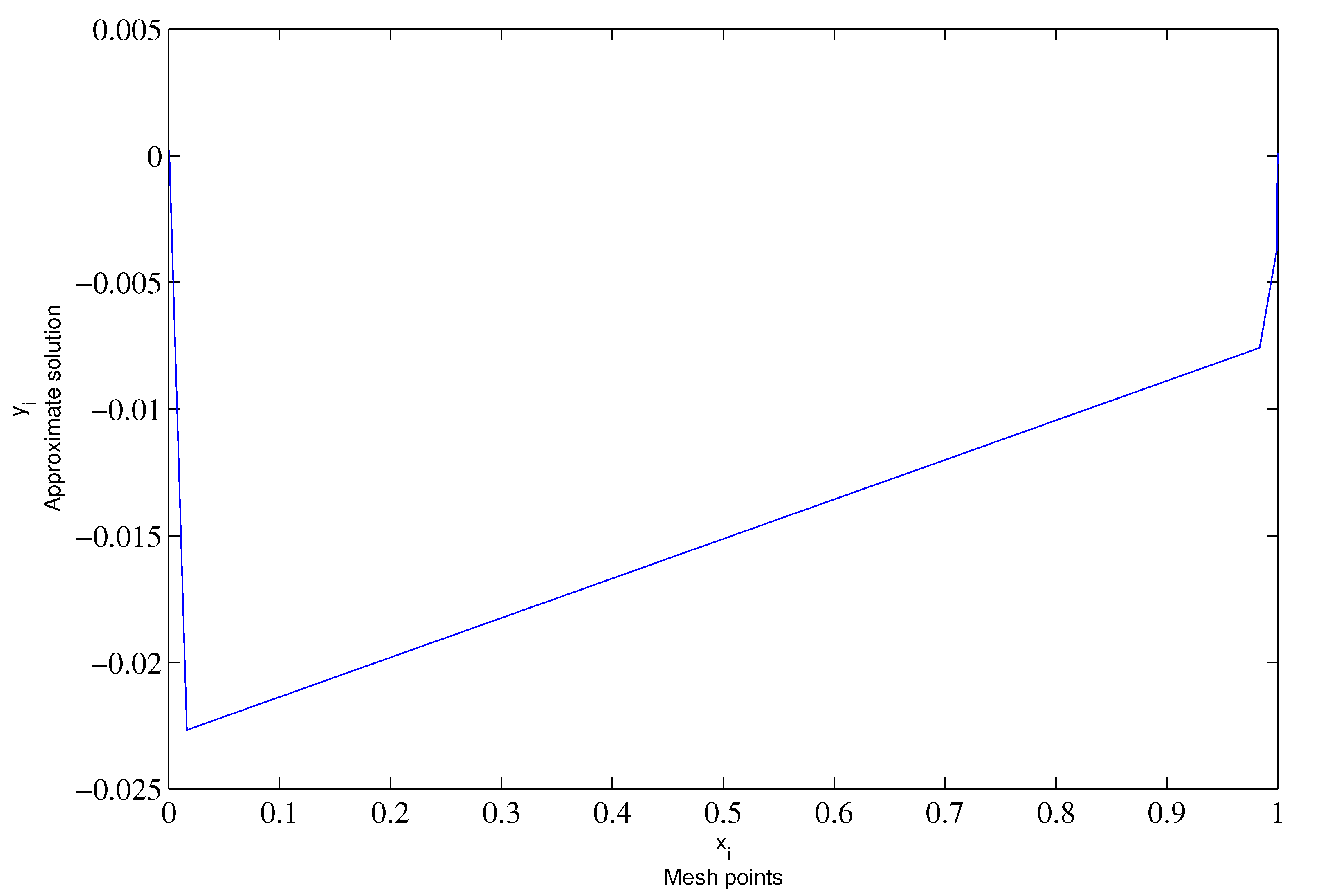
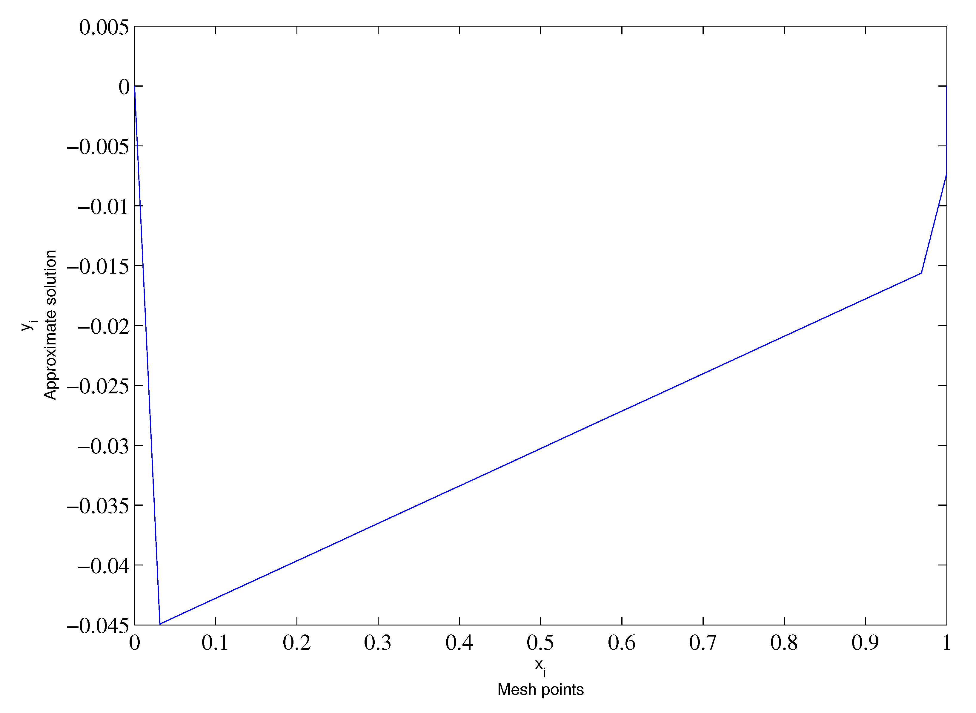
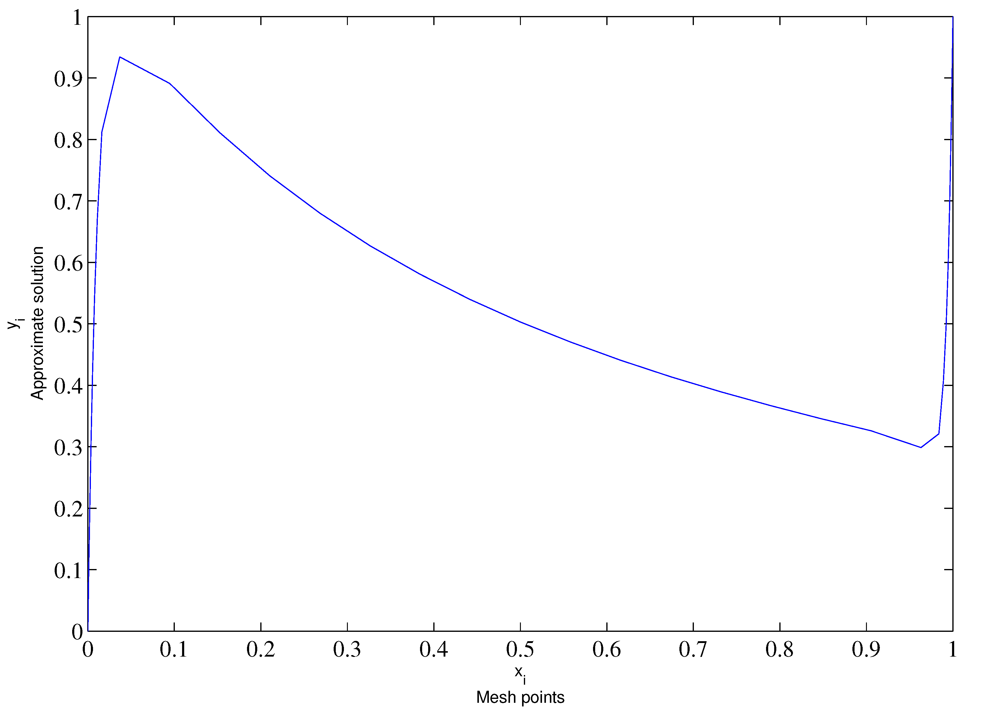
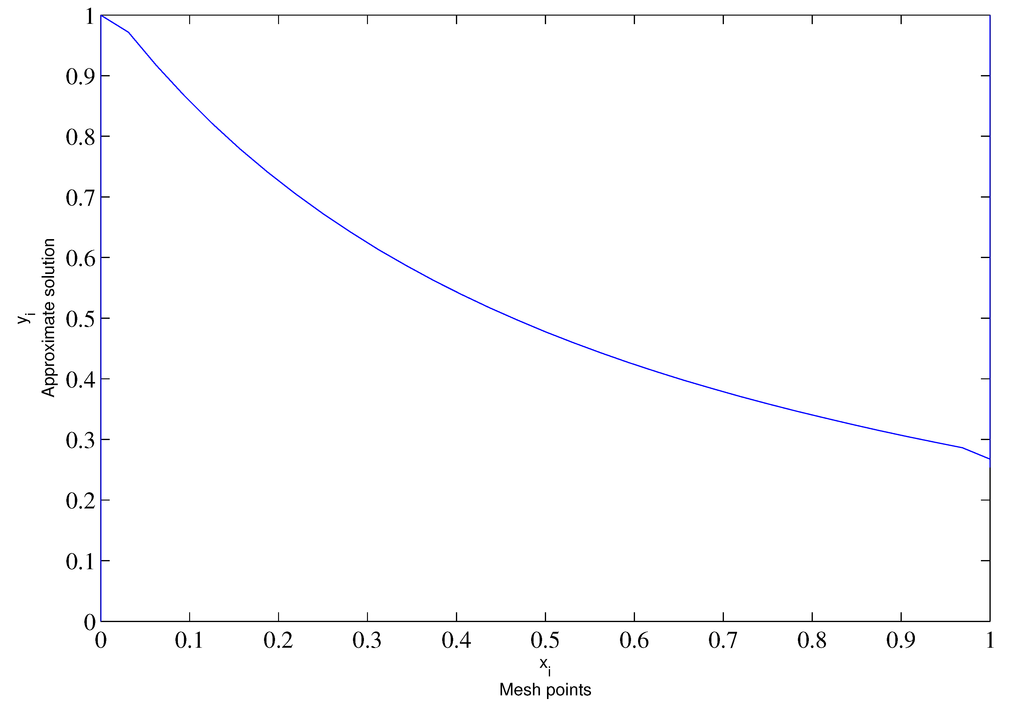
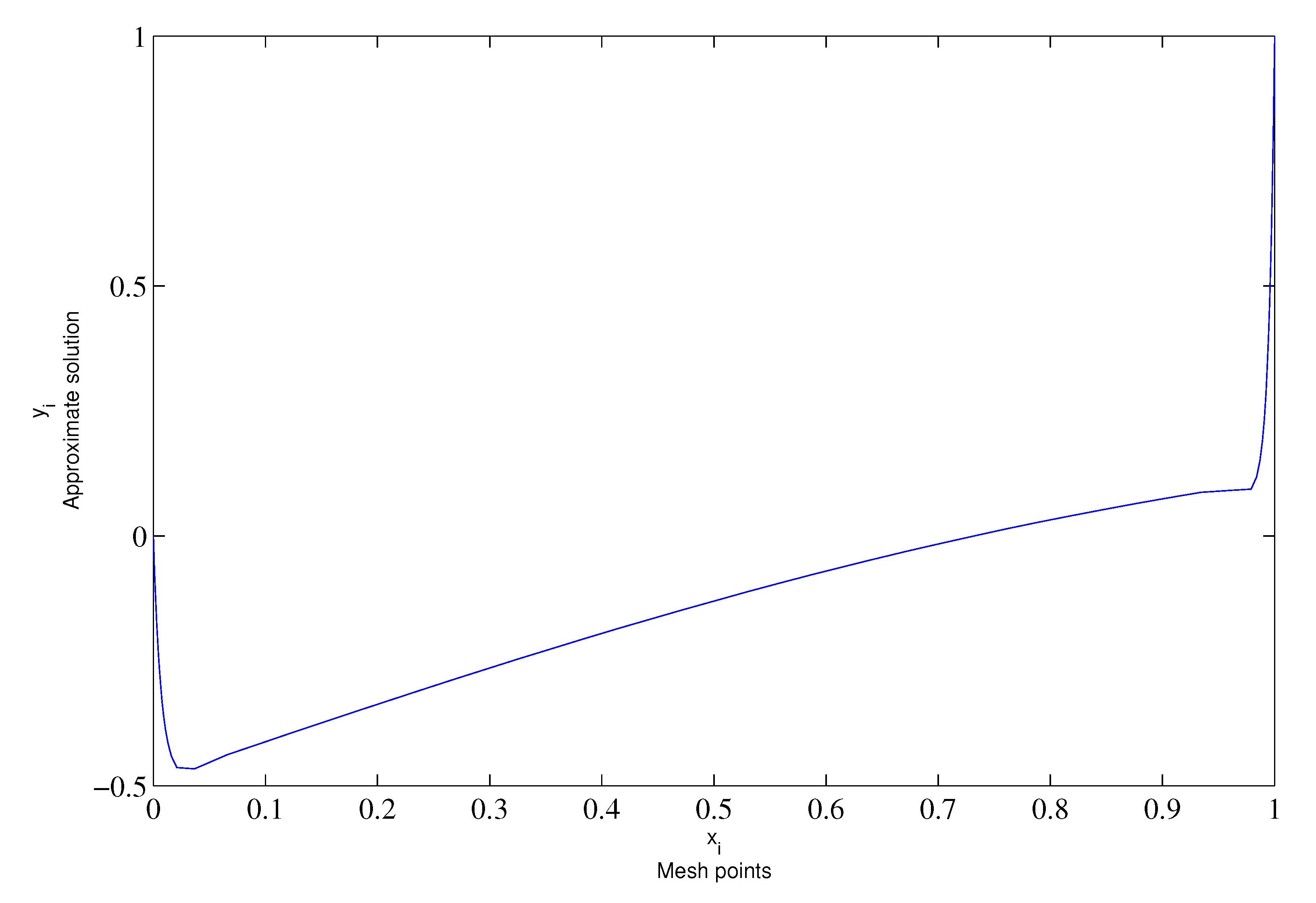
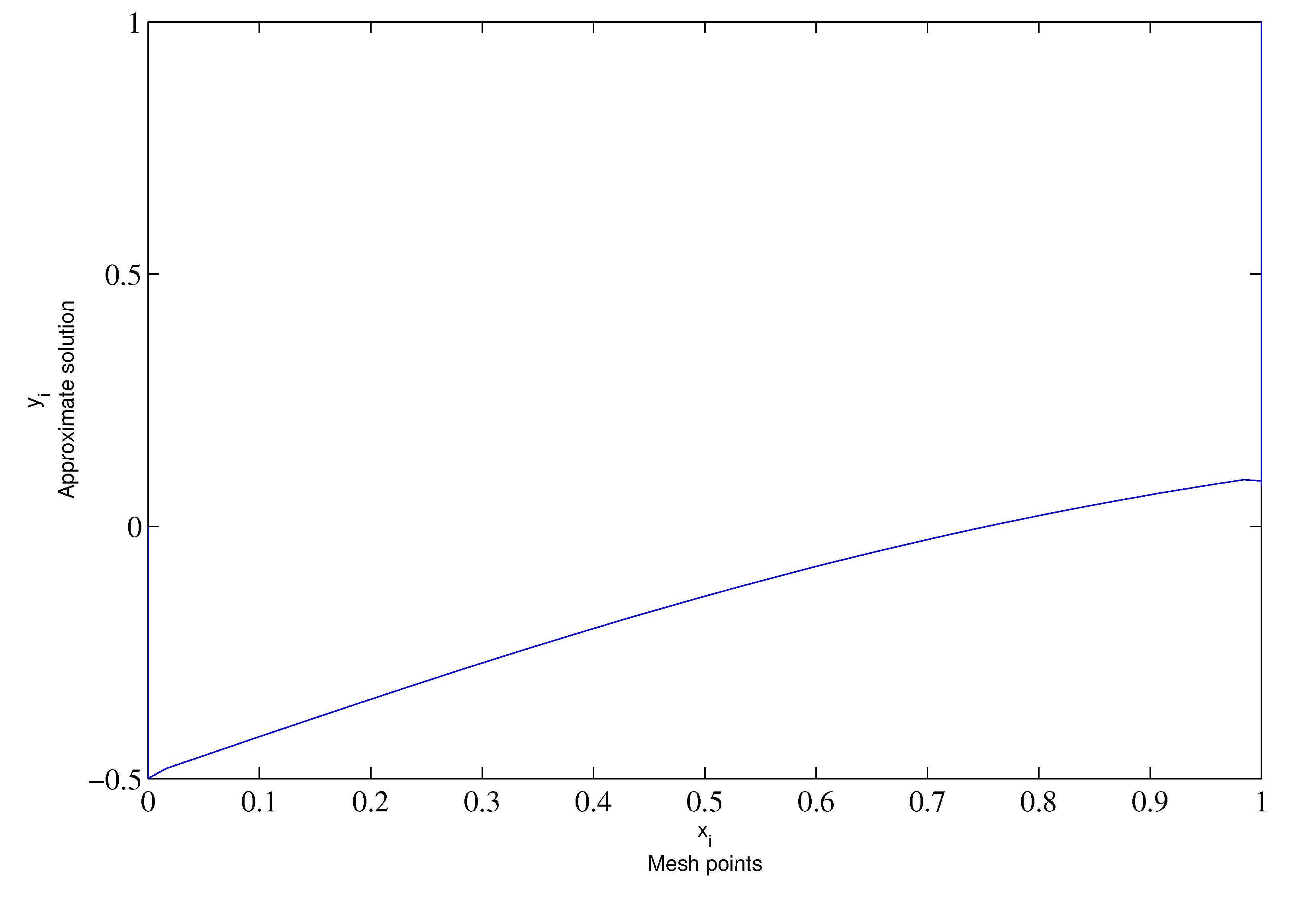
5. Results and Discussion

In this section, we test the numerical method on several examples. For this, the elimination method is used to obtain maximum pointwise errors and convergence rates. Then, the discretization (30) and (31) can be written as the following form:

$$\begin{array}{ccc}\hfill A_i{y}_{i-1}-C_i{y}_i+B_i{y}_{i+1}& =& -F_i,i=1,...,N-1,\hfill \\ \hfill y_0& =& A,y_N=B.\hfill \end{array}$$

where

$$\begin{array}{ccc}\hfill A_i& =& -{\epsilon }^2{\hslash }_i^{-1}{h}_i^{-1},B_i=-{\epsilon }^2{\hslash }_i^{-1}{h}_{i+1}^{-1},\hfill \\ \hfill C_i& =& -\left({\epsilon }^2{\hslash }_i^{-1}{h}_i^{-1}+{\epsilon }^2{\hslash }_i^{-1}{h}_{i+1}^{-1}+a_i\right),\hfill \\ \hfill F_i& =& -f_i+\lambda \sum _{j=1}^i{\hslash }_j{K}_{1,ij}{y}_j+\lambda \sum _{j=1}^N{\hslash }_j{K}_{2,ij}{y}_j.\hfill \end{array}$$

Here, the coefficients of the elimination method are as follow [45]:

$$\begin{array}{ccc}\hfill {\alpha }_{i+1}& =& \frac{B_i}{C_i-{\alpha }_i{A}_i},{\alpha }_1=0,i=1,...,N-1,\hfill \\ \hfill {\beta }_{i+1}& =& \frac{F_i+A_i{\beta }_i}{C_i-{\alpha }_i{A}_i},{\beta }_1=1,i=1,...,N-1\hfill \end{array}$$

and

$$y_i={\alpha }_{i+1}{y}_{i+1}+{\beta }_{i+1},i=N-1,\dots ,1.$$

The corresponding Algorithm 1 is given by

Algorithm 1: To compute the numerical solution $y_i$.

Input: $\epsilon$, $N$, $x\left(0\right)$ = $x0$, $x\left(l\right)$ = $xN$, $a\left(x\right)$, $f\left(x\right)$, $K_1(x,t)$, $K_2(x,t)$ and $\alpha$

Output: The numerical solution $y_i$

Step 1: ${\sigma }_1=sigma1=min((xN-x0)/4,abs((\epsilon \ast reallog\left(\epsilon \right))/\alpha ));$

${\sigma }_2=sigma2=xN-sigma1$

$h^{\left(1\right)}=h1=(sigma2-sigma1)/(N/2)$

Step 2: for $i=2:N+1$

$h_i=h\left(i\right)=x\left(i\right)-x(i-1)$

${\hslash }_i=h2\left(i\right)=(h(i+1)+h\left(i\right))/2$

end

Step 3: for $i=2:N+1$

if $\left(\right(i<=N/4+1)\&\&(sigma1<(xN-x0)/4\left)\right)$

$x\left(i\right)=-\epsilon \ast reallog(1-(1-\epsilon )\ast 4\ast (i-1)/N)/\alpha$

end

if $(i<=N/4+1)\&\&(sigma1==(xN-x0)/4)$

$x\left(i\right)=-\epsilon \ast reallog(1-(1-exp(-\alpha \ast xN/(2\ast \epsilon \left)\right))\ast 4\ast (i-1)/N)/\alpha$

end

if $\left(\right(i>N/4+1)\&\&(i<=3\ast N/4+1\left)\right)$

$x\left(i\right)=sigma1+h1\ast (i-1-N/4)$

end

if $\left(\right(i>3\ast N/4+1)\&\&(i<=N\left)\right)$

$x\left(i\right)=xN-x(N+2-i)$

end

end

Step 4: for $i=2:N$

$(A_i=A\left(i\right),$$B_i=B\left(i\right),$$C_i=C\left(i\right),$$F_i=F\left(i\right),$${\alpha }_i=alfa\left(i\right),$${\beta }_i=beta\left(i\right))$

$alfa(i+1)=B\left(i\right)./\left(C\right(i)-alfa(i).\ast A(i\left)\right);$

$beta(i+1)=\left(E\right(i)+beta(i).\ast A(i\left)\right)./\left(C\right(i)-alfa(i).\ast A(i\left)\right)$

$y\left(i\right)=y(i+1).\ast alfa(i+1)+beta(i+1)$

end

All numerical computations and figures have been carried out by Matlab R2013a. In the numerical experiments, the transition point is chosen as ${\sigma }_1\approx 0.25$.

Example 1.

Consider a particular problem

$$-{\epsilon }^2{u}^{″}+u+\underset{0}{\overset{x}{{\displaystyle \int }}}u\left(t\right)dt+\underset{0}{\overset{1}{{\displaystyle \int }}}u\left(t\right)dt=-\epsilon \left(e^{\frac{-x}{\epsilon }}+e^{\frac{-1}{\epsilon }}-2\right), x\in \left(0,1\right)$$

$$u\left(0\right)=1,u\left(1\right)=e^{\frac{-1}{\epsilon }},$$

in which the exact solution is $u\left(x\right)=e^{\frac{-x}{\epsilon }}$. The nodal maximum errors are specified as

$$e^N={\displaystyle \underset{0\le i\le N}{max}}\left|y_i-u_i\right|,$$

where $u_i$ is the exact solution and $y_i$ is approximate solution. Furthermore, the convergence rates are computed as follows

$$p^N=\frac{ln(e^N/e^{2N})}{ln2}.$$

The computed results are presented in Table 1.

Table 1. Maximum pointwise errors $e^N$ and order of convergence $p^N$ on ${\omega }_N$.

$\mathsf{\epsilon }$	$\mathit{N}=64$	$\mathit{N}=128$	$\mathit{N}=256$	$\mathit{N}=512$	$\mathit{N}=1024$
${10}^{-2}$	1.81764$\times {10}^{-2}$	$9.3384\times {10}^{-3}$	$4.73852\times {10}^{-3}$	$2.38932\times {10}^{-3}$	$1.200183-03$
	$0.96$	$0.97$	$0.98$	$0.99$
${10}^{-4}$	$2.214777\times {10}^{-2}$	$1.137744\times {10}^{-2}$	$5.76341\times {10}^{-3}$	$2.89803\times {10}^{-3}$	$1.45366\times {10}^{-3}$
	$0.97$	$0.98$	$0.98$	$0.99$
${10}^{-6}$	$2.221578\times {10}^{-2}$	$1.141305\times {10}^{-2}$	$5.78281\times {10}^{-3}$	$2.91048\times {10}^{-3}$	$1.46022\times {10}^{-3}$
	$0.97$	$0.98$	$0.99$	$0.99$
${10}^{-8}$	$2.432828\times {10}^{-2}$	$1.141356\times {10}^{-2}$	$5.78307\times {10}^{-3}$	$2.91785\times {10}^{-3}$	$1.46448\times {10}^{-3}$
	$0.97$	$0.98$	$0.99$	$0.99$
${10}^{-10}$	$2.211679\times {10}^{-2}$	$1.141357\times {10}^{-2}$	$5.78891\times {10}^{-3}$	$2.91269\times {10}^{-3}$	$1.46123\times {10}^{-3}$
	$0.97$	$0.98$	$0.98$	$0.99$
${10}^{-12}$	$2.204231\times {10}^{-2}$	$1.14026\times {10}^{-2}$	$5.7821\times {10}^{-3}$	$2.91061\times {10}^{-3}$	$1.46007\times {10}^{-3}$
	$0.97$	$0.98$	$0.99$	$0.99$
$e^N$	$2.432828\times {10}^{-2}$	$1.141357\times {10}^{-2}$	$5.78891\times {10}^{-3}$	$2.91785\times {10}^{-3}$	$1.46448\times {10}^{-3}$
$p^N$	$0.96$	$0.97$	$0.98$	$0.99$

The behavior of the numerical solution is demonstrated in Figure 1 and Figure 2.

Figure 1. Behavior of the numerical solution for $\epsilon ={10}^{-4}$ and $N=128$.

Figure 2. Numerical approximation for $\epsilon ={10}^{-12}$ and $N=64$.

From Figure 1 and Figure 2, it can be seen that the maximal errors are concentrated within the boundary layers.

Example 2.

We take into account another problem

$$-{\epsilon }^2{u}^{″}+(x+1)u+\frac{1}{2}\underset{0}{\overset{x}{\int }}(1-e^{xt})u\left(t\right)dt+\frac{1}{2}\underset{0}{\overset{1}{\int }}tu\left(t\right)dt=\frac{1}{1+x},x\in (0,1),$$

$$u\left(0\right)=0,u\left(1\right)=1.$$

The exact solution of this equation is unknown. Since the exact solution is unknown, we use the double-mesh technique. The error approximations are indicated by

$$e^N={\displaystyle \underset{0\le i\le N}{max}}\left|y_i^N-y_i^{2N}\right|$$

and the order of convergence is defined as follows

$$p^N=\frac{ln(e^N/e^{2N})}{ln2}.$$

Error approximations are shown in Table 2.

Table 2. Maximum pointwise errors $e^N$ and order of convergence $p^N$ on ${\omega }_N$.

$\mathsf{\epsilon }$	$\mathit{N}=64$	$\mathit{N}=128$	$\mathit{N}=256$	$\mathit{N}=512$	$\mathit{N}=1024$
${10}^{-2}$	2.772958$\times {10}^{-2}$	$1.392083\times {10}^{-2}$	$6.9501\times {10}^{-3}$	$3.4764\times {10}^{-3}$	$1.74087\times {10}^{-3}$
	$0.99$	$1.00$	$1.00$	$1.00$
${10}^{-4}$	$3.289871\times {10}^{-2}$	$1.64391\times {10}^{-2}$	$8.21645\times {10}^{-3}$	$4.10664\times {10}^{-3}$	$2.05148\times {10}^{-3}$
	$1.01$	$1.00$	$1.00$	$1.00$
${10}^{-6}$	$3.299511\times {10}^{-2}$	$1.648756\times {10}^{-2}$	$8.24116\times {10}^{-3}$	$4.11991\times {10}^{-3}$	$2.05978\times {10}^{-3}$
	$1.01$	$1.00$	$1.00$	$1.01$
${10}^{-8}$	$3.299655\times {10}^{-2}$	$1.648829\times {10}^{-2}$	$8.24152\times {10}^{-3}$	$4.12113\times {10}^{-3}$	$2.05604\times {10}^{-3}$
	$1.00$	$1.00$	$1.00$	$1.00$
${10}^{-10}$	$3.299657\times {10}^{-2}$	$1.648829\times {10}^{-2}$	$8.24153\times {10}^{-3}$	$4.12871\times {10}^{-3}$	$2.05987\times {10}^{-3}$
	$0.99$	$0.99$	$1.00$	$1.00$
${10}^{-12}$	$3.298523\times {10}^{-2}$	$1.64883\times {10}^{-2}$	$8.24044\times {10}^{-3}$	$4.12009\times {10}^{-3}$	$2.05139\times {10}^{-3}$
	$1.01$	$1.00$	$1.01$	$1.02$
$e^N$	$3.299657\times {10}^{-2}$	$1.648830\times {10}^{-2}$	$8.24153\times {10}^{-3}$	$4.12871\times {10}^{-3}$	$2.05987\times {10}^{-3}$
$p^N$	$0.99$	$0.99$	$1.00$	$1.00$

The computational results are reflected in the Figure 3 and Figure 4.

Figure 3. Numerical solution for $\epsilon ={10}^{-2}$ and $N=32$.

Figure 4. Behavior of the approximate solution for $\epsilon ={10}^{-12}$ and $N=64$.

In Figure 3 and Figure 4, from $\epsilon ={10}^{-2}$ to $\epsilon ={10}^{-12}$, it is seen that numerical solution behaves stable.

Example 3.

Examine the last problem

$$-{\epsilon }^2{u}^{″}+(1+e^x)u+\underset{0}{\overset{x}{\int }}sinh\left(t\right)u\left(t\right)dt+\underset{0}{\overset{1}{\int }}cosh\left(t\right)u\left(t\right)dt=sinx-cosx,x\in (0,1),$$

$$u\left(0\right)=0, u\left(1\right)=e^{\frac{-1}{\epsilon }}+1$$

The exact solution of this problem is unknown. Thus, we apply the double-mesh principle again. The obtained results are summarized in Table 3.

Table 3. Maximum pointwise errors $e^N$ and order of convergence $p^N$ on ${\omega }_N$.

$\mathsf{\epsilon }$	$\mathit{N}=64$	$\mathit{N}=128$	$\mathit{N}=256$	$\mathit{N}=512$	$\mathit{N}=1024$
${10}^{-2}$	1.233841$\times {10}^{-2}$	$6.29078\times {10}^{-3}$	$3.16786\times {10}^{-3}$	$1.59413\times {10}^{-3}$	$8.0295\times {10}^{-4}$
	$0.97$	$0.99$	$0.99$	$0.99$
${10}^{-4}$	$1.511043\times {10}^{-2}$	$7.66589\times {10}^{-3}$	$3.8615\times {10}^{-3}$	$1.93738\times {10}^{-3}$	$9.6936\times {10}^{-4}$
	$0.98$	$0.99$	$0.99$	$1.00$
${10}^{-6}$	$1.516372\times {10}^{-2}$	$7.69353\times {10}^{-3}$	$3.87596\times {10}^{-3}$	$1.90705\times {10}^{-3}$	$9.3596\times {10}^{-4}$
	$0.97$	$0.99$	$1.02$	$1.02$
${10}^{-8}$	$1.516452\times {10}^{-2}$	$7.69395\times {10}^{-3}$	$4.03036\times {10}^{-3}$	$1.92596\times {10}^{-3}$	$9.1215\times {10}^{-4}$
	$0.97$	$0.93$	$1.06$	$1.07$
${10}^{-10}$	$1.516453\times {10}^{-2}$	$7.69487\times {10}^{-3}$	$4.03738\times {10}^{-3}$	$1.94571\times {10}^{-3}$	$9.0143\times {10}^{-4}$
	$0.98$	$0.93$	$1.05$	$1.11$
${10}^{-12}$	$1.516204\times {10}^{-2}$	$7.69318\times {10}^{-3}$	$3.83764\times {10}^{-3}$	$1.9232\times {10}^{-3}$	$9.0138\times {10}^{-4}$
	$0.98$	$1.00$	$1.00$	$1.09$
$e^N$	$1.516453\times {10}^{-2}$	$7.69487\times {10}^{-3}$	$4.03764\times {10}^{-3}$	$1.93571\times {10}^{-3}$	$9.6936\times {10}^{-4}$
$p^N$	$0.97$	$0.93$	$0.99$	$0.99$

The improvement in the numerical solution within the boundary layers is illustrated in Figure 5 and Figure 6.

Figure 5. Numerical approximation for $\epsilon ={10}^{-2}$ and $N=64$.

Figure 6. Numerical behavior for $\epsilon ={10}^{-10}$ and $N=128$.

Figure 5 and Figure 6 show that the numerical solution is treated as $\epsilon$ decreases.

In summary, from Table 1, Table 2 and Table 3, as N increases, maximum pointwise errors decrease and the order of uniform convergence of the presented difference scheme is almost 1. It can be concluded that the presented difference scheme yields stable and uniform numerical results. Moreover, from Figure 1, Figure 2, Figure 3, Figure 4, Figure 5 and Figure 6, it is seen that the numerical solution curves converge to the coordinate axes for smaller values of $\epsilon$. Thus, the proposed method seems to be effective for solving such problems.

6. Concluding Remarks

In this paper, we suggested a new and stable difference scheme for solving boundary value problems of singularly perturbed second-order Volterra–Fredholm integro-differential equations. The stability and convergence of the method were examined in the discrete maximum norm. The effectiveness and reliability of the presented scheme are demonstrated by three numerical examples. The computed results reveal that the order of convergence was found as $O\left(N^{-1}\right).$ Namely, the scheme is first-order accurate. Although the proposed method is reliable, the order of convergence of the numerical scheme may need to be improved. In order to expand numerical research, experiments in which improvements in the order and different boundary conditions (i.e., nonlocal, integral, Robin, and mixed) can be considered.

References

- Amin, R.; Nazir, S.; Garcia-Magarino, I. A collocation method for numerical solution of nonlinear delay integro-differential equations for wireless sensor network and internet of things. Sensors 2020, 20, 1962. [Google Scholar] [CrossRef] [PubMed]
- Dawood, L.A.; Hamoud, A.; Mohammed, N.M. Laplace discrete decomposition method for solving nonlinear Volterra-Fredholm integro-differential equations. J. Math. Comput. Sci. 2020, 21, 158–163. [Google Scholar] [CrossRef]
- Kashkaria, B.S.H.; Syam, M.I. Evolutionary computational intelligence in solving a class of nonlinear Volterra-Fredholm integro-differential equations. J. Comput. Applied Math. 2017, 311, 314–323. [Google Scholar] [CrossRef]
- Bellomo, N.; Firmani, B.; Guerri, L. Bifurcation analysis for a nonlinear system of integro-differential equations modelling tumor-immune cells competition. Appl. Math. Lett. 1999, 12, 39–44. [Google Scholar] [CrossRef]
- Guan, L.; Prieur, C.; Zhang, L.; Prieur, C.; Georges, D.; Bellemain, P. Transport effect of Covid-19 pandemic in France. Annu. Rev. Control 2020, 50, 394–408. [Google Scholar] [CrossRef]
- Köhler-Rieper, F.; Röhl, C.H.F.; De Michecli, E. A novel deterministic forecast model for the Covid-19 epidemic based on a single ordinary integro-differential equations. Eur. Phys. J. Plus 2020, 135, 599. [Google Scholar] [CrossRef]
- Hamoud, A.A.; Bani Issa, M.; Ghadle, K.P. Existence and uniqueness results for nonlinear Volterra-Fredholm integro-differential equations. Nonlinear Funct. Anal. Appl. 2018, 23, 797–805. [Google Scholar]
- Hamoud, A.; Mohammed, N.; Ghadle, K. Existence and uniqueness results for Volterra-Fredholm integro-differential equations. Adv. Theory Nonlinear Anal. Appl. 2020, 4, 361–372. [Google Scholar] [CrossRef]
- Al-Ahmad, S.; Sulaiman, I.M.; Nawi, M.M.A.; Mamat, M.; Ahmad, M.Z. Analytical solution of systems of Volterra integro-differential equations using modified differential transform method. J. Math. Comput. Sci. 2022, 26, 1–9. [Google Scholar] [CrossRef]
- Bani Issa, M.S.H.; Hamoud, A.A. Solving systems of Volterra integro-differential equations by using semi analytical techniques. Technol. Rep. Kansai Univ. 2020, 62, 685–690. [Google Scholar]
- Tahernezad, T.; Jalilian, R. Exponential spline for the numerical solutions of linear Fredholm integro-differential equations. Adv. Differ. Equations 2020, 141, 1–15. [Google Scholar] [CrossRef]
- Segni, S.; Ghiat, M.; Guebbai, H. New approximation method for Volterra nonlinear integro-differential equations. Asian-Eur. J. Math. 2019, 12, 1950016. [Google Scholar] [CrossRef]
- Alvandi, A.; Paripour, M. The combined reproducing kernel method and Taylor series for handling nonlinear Volterra integro-differential equations with derivative type kernel. Appl. Math. Comput. 2019, 355, 151–160. [Google Scholar] [CrossRef]
- Amin, R.; Maharq, I.; Shah, K.; Elsayed, F. Numerical solution of the second order linear and nonlinear integro-differential equations using Haar wavelet method. Arab. J. Basic Appl. Sci. 2021, 28, 1–19. [Google Scholar] [CrossRef]
- Swaidan, W.; Ali, H.S. A computational method for nonlinear Fredholm integro-differential equations using Haar wavelet collocation points. J. Physics Conf. Ser. 2021, 1, 012032. [Google Scholar] [CrossRef]
- Issa, K.; Salehi, F. Approximate solution of perturbed Volterra-Fredholm integro-differential equations by Chebyshev Galerkin method. J. Math. 2017, 2017, 8213932. [Google Scholar] [CrossRef]
- Basirat, B.; Shahdadi, M.A. Numerical solution of nonlinear integro-differential equations with initial conditions by Bernstein Operational matrix of derivative. Int. J. Mod. Nonlinear Theory Appl. 2013, 2, 141–149. [Google Scholar] [CrossRef]
- Cakir, M.; Gunes, B.; Duru, H. A novel computational method for solving nonlinear Volterra integro-differential equation. Kuwait J. Sci. 2021, 48, 31–40. [Google Scholar] [CrossRef]
- Cimen, E.; Yatar, S. Numerical solution of Volterra integro-differential equtaion with delay. J. Math. Comput. Sci. 2020, 20, 255–263. [Google Scholar] [CrossRef]
- Chen, J.; He, M.; Huang, Y. A fast multiscale Galerkin method for solving second order linear Fredholm integro-differential equation with Dirichlet boundary conditions. J. Comput. Appl. Math. 2020, 364, 112352. [Google Scholar] [CrossRef]
- Hesameddini, E.; Riahi, M. Galerkin matrix method and its convergence analysis for solving system of Volterra-Fredholm integro-differential equations. Iran. J. Sci. Technol. Sci. 2019, 43, 1203–1214. [Google Scholar] [CrossRef]
- Ghomanjani, F. Numerical solution for nonlinear Volterra integro-differential equations. Palest. J. Math. 2020, 9, 164–169. [Google Scholar]
- Cao, Y.; Nikan, O.; Avazzadeh, Z. A localized meshless technique for solving 2D nonlinear integro-differential equation with multi-term kernels. Appl. Numer. Math. 2023, 183, 140–156. [Google Scholar] [CrossRef]
- Jafarzadeh, Y.; Ezzati, R. A new method for the solution of Volterra-Fredholm integro-differential equations. Tblisi Math. J. 2019, 12, 59–66. [Google Scholar] [CrossRef]
- Sharif, A.A.; Hamoud, A.A.; Ghadle, K.P. Solving nonlinear integro-differential equations by using numerical techniques. Acta Univ. Apulensis 2020, 61, 43–53. [Google Scholar]
- Shoushan, A.F.; Al-Humedi, H.O. The numerical solutions of integro-differential equations by Euler polynomials with least-squares method. Polarch J. Archaeol. Egypt/Egyptol. 2021, 18, 1740–1753. [Google Scholar]
- Iragi, B.C.; Munyakazi, J.B. New parameter-uniform discretizations of singularly perturbed Volterra integro-differential equations. Appl. Math. Int. Sci. 2018, 12, 517–529. [Google Scholar] [CrossRef]
- Iragi, B.C.; Munyakazi, J.B. A uniformly convergent numerical method for a singularly perturbed Volterra integro-differential equation. Int. J. Comput. Math. 2020, 97, 759–771. [Google Scholar] [CrossRef]
- Kudu, M.; Amirali, I.; Amiraliyev, G.M. A finite difference method for a singularly perturbed delay integro-differential equations. J. Of Computational Appl. Math. 2016, 308, 379–390. [Google Scholar] [CrossRef]
- Yapman, Ö.; Amiraliyev, G.M.; Amirali, I. Convergence analysis of fitted numerical method for a singularly perturbed nonlinear Volterra integro-differential equation with delay. J. Comput. And Applied Math. 2019, 355, 301–309. [Google Scholar] [CrossRef]
- Amiraliyev, G.M.; Yapman, Ö.; Kudu, M. A fitted approximate method for a Volterra delay-integro-differential equation with initial layer. Hacet. J. Math. Stat. 2019, 48, 1417–1429. [Google Scholar] [CrossRef]
- Mbroh, N.A.; Noutchie, S.C.O.; Massoukou, R.Y.M. A second order finite difference scheme for singularly perturbed Volterra integro-differential equation. Alex. Eng. J. 2020, 59, 2441–2447. [Google Scholar] [CrossRef]
- Yapman, Ö.; Amiraliyev, G.M. A novel second order fitted computational method for a singularly perturbed Volterra integro-differential equation. Int. J. Comput. Math. 2019, 97, 1293–1302. [Google Scholar] [CrossRef]
- Tao, X.; Zhang, Y. The coupled method for singularly perturbed Volterra integro-differential equations. Adv. Differ. Equations 2019, 217, 2139. [Google Scholar] [CrossRef]
- Panda, A.; Mohapatra, J.; Amirali, I. A second-order post-processing technique for singularly perturbed Volterra integro-differential equations. Mediterr. J. Math. 2021, 18, 1–25. [Google Scholar] [CrossRef]
- Amiraliyev, G.M.; Durmaz, M.E.; Kudu, M. Uniform convergence results for singularly perturbed Fredholm integro-differential equation. J. Of Mathematical Anal. 2018, 9, 55–64. [Google Scholar]
- Amiraliyev, G.M.; Durmaz, M.E.; Kudu, M. Fitted second order numerical method for a singularly perturbed Fredholm integro-differential equations. Bull. Belg. Math. Soc. Simon Stevin 2020, 27, 71–88. [Google Scholar] [CrossRef]
- Cimen, E.; Cakir, M. A uniform numerical method for solving singularly perturbed Fredholm integro-differential problem. Comput. Appl. Math. 2021, 40, 1–14. [Google Scholar] [CrossRef]
- Durmaz, M.E.; Amiraliyev, G.M. A robust numerical method for a singularly perturbed Fredholm integro-differential equation. Mediterr. J. Math. 2021, 18, 1–17. [Google Scholar] [CrossRef]
- Cakir, M.; Gunes, B. Exponentially fitted difference scheme for singularly perturbed mixed integro-differential equations. Georgian Math. J. 2022, 29, 193–203. [Google Scholar] [CrossRef]
- Cakir, M.; Gunes, B. A new difference method for the singularly perturbed Volterra-Fredholm integro-differential equations on a Shishkin mesh. Hacet. J. Math. Stat. 2022, 51, 787–799. [Google Scholar]
- Amiraliyev, G.M.; Durmaz, M.E.; Kudu, M. A numerical method for a second order singularly perturbed Fredholm integro-differential equation. Miskolc Math. Notes 2021, 22, 37–48. [Google Scholar]
- Boglaev, I.P. Approximate solution of a nonlinear boundary value problem with a small parameter for the highest-order differential. USSR Comput. Math. Math. Phys. 1984, 24, 30–35. [Google Scholar] [CrossRef]
- Amiraliyev, G.M.; Mamedov, Y.D. Difference schemes on the uniform mesh for singularly perturbed pseudo-parabolic equations. Tr. J. Math. 1995, 19, 207–222. [Google Scholar]
- Samarski, A.A. The Theory of Difference Schemes; M.V. Lomonosov State University: Moscow, Russia, 2021. [Google Scholar]
Publisher’s Note: MDPI stays neutral with regard to jurisdictional claims in published maps and institutional affiliations. |
© 2022 by the authors. Licensee MDPI, Basel, Switzerland. This article is an open access article distributed under the terms and conditions of the Creative Commons Attribution (CC BY) license (https://creativecommons.org/licenses/by/4.0/).