Abstract
Aiming at the problem that the toe cap and upper part of the sole of a shoe easily appear missing when using binocular vision to reconstruct the shoe sole in the industrial production process, an improved matching cost calculation method is proposed to reconstruct shoe soles in three dimensions. Firstly, a binocular vision platform is built, and Zhang’s calibration method is used to obtain the calibration parameters. Secondly, the method of fusing Census and BT costs is used to calculate the matching cost of the image, so that the matching cost calculation result is more accurate. On this basis, 4-path aggregation is performed on the obtained cost, and the optimal matching cost is selected in combination with the WTA algorithm. Finally, left–right consistency detection and median filtering are used to optimize the disparity map and combine the camera calibration parameters to reconstruct the shoe sole in three dimensions. The experimental results show that the average mismatch rate of the four images on the Middlebury website in this method is about 6.57%, the reconstructed sole point cloud contour information is complete, and there is no material missing at the toe and heel.
MSC:
68U10
1. Introduction
In recent years, with rising labor costs and the development of automation technology, footwear manufacturers have begun to seek automated production of key processes in the shoemaking process [1,2]. Sole gluing is a key process in shoemaking and one that greatly affects the quality and aesthetics of shoes. In the past, sole gluing was mostly done by hand, and the volatile gas from shoe glue threatened the health of workers. Moreover, because the quality of glue applied by workers with different proficiency levels is accordingly different, more and more shoe enterprises are using robots for sole gluing instead of relying on manual operation [3]. A three-dimensional model of the sole can be obtained by 3D reconstruction, which lays a foundation for the extraction of the sole glue track. Therefore, it is of great significance to study how to use machine vision technology to realize 3D reconstruction of soles for shoe enterprises to realize automatic production.
Nowadays, machine vision technology is being gradually introduced into automatic gluing equipment. At present, most sole gluing equipment uses line-laser or binocular- structured light to reconstruct the sole in three dimensions, but the cost of line-laser and structured light is relatively high [4]. Monocular vision is affected by factors such as angle of view, and the reconstruction accuracy is low. Binocular vision can better balance hardware cost and reconstruction accuracy. At present, how to use a binocular stereo matching algorithm for 3D reconstruction of soles and improve the accuracy and speed of the algorithm has become a hot issue in the field of machine vision. Relevant scholars have conducted much research and achieved fruitful results [5,6,7]. On the basis of binocular vision, Li Zhenzhen et al. [8] added LED light bars, increased the contrast of sole edges, and used the edge stereo matching method for feature matching. Experiments show that the sole edges obtained by this method are relatively complete. Ding Dukun et al. [9] adopted the threshold segmentation method based on a genetic algorithm. The experimental results show that compared with traditional methods, this method has stronger anti-interference and more accurate sole information extraction. Stefano Pagano et al. [10] used a Kinect V2 vision system to obtain point cloud data of soles and designed trajectory extraction algorithms for planar 2D objects and 3D objects, which improved the flexibility of the bonding process. Zhu et al. [11] transformed the spatial trajectory of the sole into a two-dimensional image depth map, extracted the edge contour of the sole by a two-block algorithm, and fitted and biased the contour line by B spline to obtain the spraying trajectory. Ma Xinwu et al. [12] used a canny algorithm to extract the edge of the sole and used a region-matching algorithm for stereo matching. The cubic spline interpolation was performed on the obtained three-dimensional contour line of the sole, and the glue spraying trajectory was obtained through offset. Experiments have shown that this method has good real-time performance. Luo Jiufei et al. [13] used the accelerated robust feature algorithm and the adaptive double threshold algorithm to extract initial matching pairs in left and right images, and then used distance and angle features to eliminate false matching points. Experiments have shown that the running time of this method is reduced by 40% compared with traditional methods, and the matching accuracy is higher. Yan Jia et al. [14] used a Sobel operator to extract edge information as the basis of the Census window, used the selected window to calculate the similarity cost and gradient information cost, and fused to obtain the cost matching function. Experimental results show that this method has better matching results for areas with inconspicuous texture and large depth change. Xiao Hong et al. [15] fused the gradient cost with the Census cost with the neighborhood pixel weight, and used guided filtering for cost aggregation. Experimental results show that this method can make full use of the coarse information and fine information of images, but the matching details need to be improved. Yu Chunhe et al. [16] aimed at the problem that points with high similarity tend to cause mismatching in the matching process, and used an SAD algorithm with different sizes of windows to deal with this problem. Experimental results show that the feature point matching of this method is more accurate. Zhu Jianhong et al. [17] added a third state to the traditional Census algorithm and used guided filtering for cost aggregation. Experimental results show that the time of this method is shortened by 36.60% compared with the traditional Census algorithm. Lim et al. [18] proposed a fast stereo matching algorithm based on Census transformation. The experimental results show that this method can resist radiation changes well, and the mismatching rate and running efficiency are improved compared with the traditional Census algorithm. Jia Kebin et al. [19] used a neighborhood information constraint algorithm to carry out weighted average processing of neighborhood center points, and used an adaptive color window for cost aggregation. Experiments have shown that this method has a low mismatching rate and strong anti-interference to Gaussian noise.
The above scholars have conducted much research on the extraction and 3D reconstruction of the sole gluing track [20,21] and have achieved fruitful results. However, most algorithms have high requirements on the color and texture of objects, and the matching effect is poor for objects with a single color and less texture, such as soles. Since the feature matching–based method often has missing trajectories at the toe and heel, this paper proposes an improved stereo matching method on the basis of the above research. In this paper, the algorithm that fuses Census and BT cost is used to calculate the matching cost to reduce the error caused by single-matching cost. The four-path aggregation strategy is used to aggregate the cost to improve the real-time performance of the algorithm. Left–right consistency detection and median filtering are used to optimize the disparity. Finally, the sole is reconstructed according to the calibration parameters.
2. Improved Binocular Visual Matching Cost Method
In order to realize the 3D reconstruction of the sole, this paper proposes a method to improve the accuracy of sole contour extraction on the premise of reducing hardware cost. In this paper, a binocular vision sole 3D reconstruction algorithm with improved matching cost is studied, and its flow is shown in Figure 1.
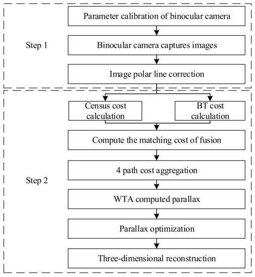
Figure 1.
Algorithm flow chart of this paper.
It can be seen from Figure 1 that the 3D reconstruction algorithm of a binocular vision sole with improved matching cost has two main steps. The first step is to build a binocular vision system, use the Zhang calibration method to obtain camera parameters, and collect sole images for polar line correction. The second step is to perform stereo matching on the image. The specific steps are as follows: First, the algorithm combining BT and Census costs is used to calculate the matching cost, and the 4-path aggregation strategy is used to aggregate the cost. The obtained disparity is then post-processed using the WTA algorithm to select the final matching cost. Finally, according to the calibrated camera parameters, 3D reconstruction of the sole is performed.
2.1. Binocular Vision Image Acquisition
2.1.1. Matching Cost Calculation
Firstly, the experimental platform of the binocular camera is built, and the Zhang calibration method is used for joint calibration. In order to ensure the accuracy of the calibration parameters, an alumina calibration plate with a side length of 5 mm is used for each small square. A total of 24 pairs of calibration images are collected, and image pairs with large errors are removed. For example, samples with large calibration offsets need to be removed. Sixteen samples are used to calibrate the image, and the calibration picture is shown in Figure 2.
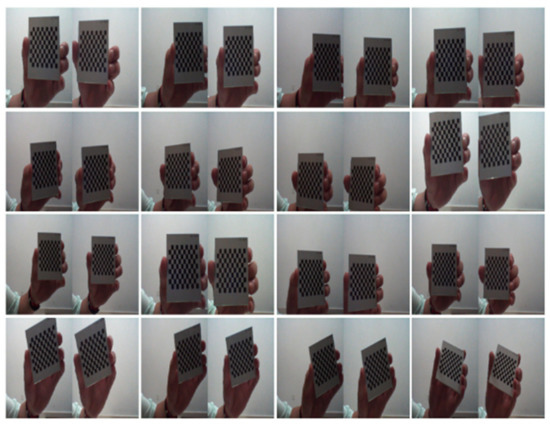
Figure 2.
Partially calibrated pictures of the camera.
Use the calibration toolbox that comes with Matlab2018b to calibrate the camera. The external parameters of the camera are shown in Table 1. The internal parameters of the camera are shown in Table 2.

Table 1.
Camera external parameter table.
Table 2.
Camera internal parameter table.
2.1.2. Binocular Vision Image Acquisition and Preprocessing
Binocular vision is widely used in the industry. It uses the left and right cameras to obtain images with differences, then calculates the parallax of the object, and finally obtains the 3D information of the object to be measured according to the camera parameters. In an ideal situation, the parameters of the two cameras are exactly the same and the imaging planes coincide. The schematic diagram is shown in Figure 3:
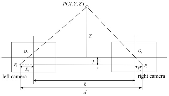
Figure 3.
Principle diagram of ideal binocular vision imaging.
Where represents the target point to be measured, and its coordinate is . and are the optical centers of the left and right cameras, respectively. is the corresponding projection point of the target point on the left image plane, and its coordinate is . is the corresponding projection point of the target point on the right image plane, and its coordinate is . is the deviation between the two positions, called parallax. is the distance between the optical center plane and the image plane, called the focal length. is the baseline distance. is the distance from point to the plane of the optical center, called the object distance. It can be seen from Figure 3 that:
The projection distance of the target on the left and right image planes is:
where and represent the projection distance of the target on the left and right image planes, respectively.
According to the similarity principle of triangles, the relationship between object distance and parallax satisfies:
After simplification, we get:
From the object distance , we can derive the other two coordinates of the point in the world coordinate system.
In the stereo matching algorithm, the points to be matched in the left image need to be matched with their corresponding points in the right image. Performing a two-dimensional search for all the pixels in the image on the right would take a long time. Therefore, the epipolar line constraint is adopted to make the corresponding two epipolar lines of the left and right images lie on the same horizontal line. In this way, you only need to search on the polar line corresponding to the right picture. Operations on a two-dimensional plane become operations on a one-dimensional line. This method greatly speeds up the operation. The image after epipolar correction is shown in the Figure 4.
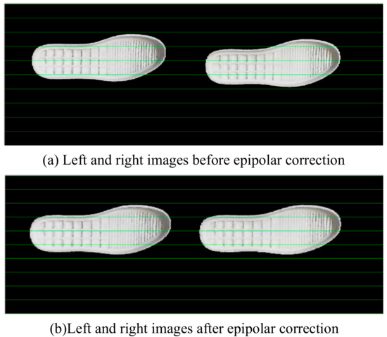
Figure 4.
Images before and after epipolar correction.
For the convenience of observing the changes before and after the epipolar correction, equidistant horizontal straight lines are added to the figure. It can be seen from Figure 4 that the points on the edge of the sole are already at the same level after the epipolar correction.
2.2. 3D reconstruction of Improved Matching Cost Algorithm
After camera calibration and epipolar correction, the camera is used to capture left and right images of the shoe sole. In order to obtain the depth information of the sole, we need to find one-to-one corresponding pixels in the two images, and obtain the disparity map by calculating the difference between these corresponding coordinates. This process is called stereo matching.
2.2.1. Match Cost Calculation
Using only a single matching cost in the matching cost calculation usually has drawbacks. For example, the cost of BT (Birchfield & Tomasi) and Sum of Absolute Differences (SAD) relies too much on grayscale information. The Census cost relies too much on the center pixel. The sole has a single color with less texture. Therefore, it is difficult to obtain good results with a single matching cost. In order to solve this problem, the BT cost is added to the Census cost for fusion to solve the problem of depth discontinuity. In this way, the calculated matching cost is more accurate.
The Census cost compares the gray value of the center point and the other points in the neighborhood window of the point to be matched in the left and right images. This is as shown in Formula (7):
where represents the gray value of the center point ; represents the gray value of other points in the field; and the center point gray value of is used as the reference value. If a point in the neighborhood is greater than , it is recorded as 0; otherwise it is recorded as 1. After the pixels in the neighborhood are compared, the points in the neighborhood are arranged in order. A binary string can then be obtained. The calculation formula is shown in Formula (8):
where represents the string corresponding to the center point, means bitwise concatenation operation, and represents the neighborhood of center point .
The bitwise XOR and bitwise sum operations of the strings obtained in the left and right images are used to obtain the Hamming distance, which is used as the cost between the two pixels. The formula is as follows:
where represents the Census matching cost; represents the corresponding string in the left image when the parallax is ; and represents the corresponding string in the right image when the parallax is . The dimension of the Census matching cost is .
BT cost is similar to SAD cost. Both are calculated using the absolute value of the grayscale difference in the pixels, but the BT cost also performs half-pixel interpolation on the two pixels. Taking the horizontal direction as an example, its schematic diagram is shown in Figure 5.
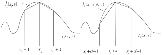
Figure 5.
BT cost interpolation principal diagram.
The calculation formula of BT cost is shown in Formula (10):
where represents the BT matching cost, represents the gray value of the pixel in the left image, and represents the gray value of the pixel in the right image, represents the grayscale value at the subpixel in the left image, and represents the grayscale value at the subpixel in the image on the right. Among them, . The grayscale value is calculated for the subpixel location between pixels and in the left image. The grayscale value is calculated for the sub-pixel location between pixels and in the right figure. The BT cost calculation is divided into two types because there are two left and right images.
There is a difference between the initial costs due to the adopted matching costs. Therefore, the difference needs to be normalized first and then fused. The normalized formula is:
The normalized matching cost is fused and multiplied by the corresponding scale factor to obtain Formula (12).
Formulas (11) and (12) can be obtained simultaneously:
where represents the normalization function; means matching cost; and represents the corresponding scale factor, which is used to assign the weight of the two costs. In order to balance the three costs, it has been debugged many times. Finally choose , .
The steps of the proposed matching cost calculation method are as follows:
- (1)
- With the point in the left figure as the center, build a neighborhood window of size .
- (2)
- Do the same operation in the right image, and select all the pixels in the right image window at the same time.
- (3)
- Compare the gray value of the left and right neighborhood center points and the other points, respectively. Obtain two binary strings according to the size of the gray value. Find the Hamming distance between the two strings to get the cost .
- (4)
- Calculate the sub-pixel interpolation of the center point of the left and right neighborhoods and the focus of the adjacent pixels, respectively. The cost can be obtained.
- (5)
- Normalize and . Fuse them according to the corresponding scale factor. The matching cost can then be obtained.
- (6)
- Repeat steps 2 to 5 until the parallax search range is exceeded.
- (7)
- Select the neighborhood with the smallest matching cost within the disparity range of the right image. The corresponding center point is the pixel that matches the points.
2.2.2. Cost Aggregation
After calculating the initial matching cost, if the disparity calculation is performed directly, the effect is generally poor. In order to improve the accuracy and robustness of stereo matching, cost aggregation is required. A scanline optimization method is used for cost aggregation.
Firstly, a global energy optimization strategy is used to find the minimized energy function. The optimal aggregation cost can then be found. The energy function formula is as follows:
where represents the disparity of pixel pointsm represents the parallax of pixels, and and represent penalty coefficients. The first term on the right side of Equation (14) represents the sum of the matching costs of all pixels when the disparity is . The second and third terms indicate that all pixels in the neighborhood of pixel are penalized. Among them,. When the parallax change is 1, is used for punishment, and when the parallax change is greater than 1, is used for punishment.
A common scheme in path aggregation is 8-path aggregation. This scheme calculates the matching cost from 8 directions, and has higher accuracy but longer operation time. Compared with the 8-path aggregation, the 4-path aggregation eliminates the four-direction paths of 5, 6, 7, and 8. Its matching speed is greatly accelerated. The strategies for 8-path aggregation and 4-path aggregation are shown in Figure 6. The calculation formula of the path cost of a pixel along a certain direction is shown in (15):
where represents the aggregation cost of disparity and pixel under the condition of path . represents the match cost value for pixel . The second term on the right side of the formula indicates that the aggregation cost on path is the value corresponding to the minimum cost when no penalty or and penalties are applied. The third term exists to prevent the path cost from being too large.

Figure 6.
Schematic diagram of 8 and 4 path aggregation.
The aggregation cost in the four directions is:
where represents the total aggregation cost, which is the sum of the four directions of 1, 2, 3, and 4. The dimension of the aggregate cost value is .
2.2.3. Parallax Optimization
After the cost aggregation for all 4 directions is obtained, the disparity corresponding to the smallest aggregated cost per pixel is used to calculate the disparity map. The winner-takes-all (WTA) algorithm is used to select the optimal cost from all possible matching costs. First, the corresponding cost value of a point in the image under all parallax is calculated. Then the smallest cost value is found via WTA. This is the optimal parallax . Subsequently, the picture taken by the left camera is used. The picture information corresponding to each point is replaced with its relative for storage. The resulting picture is the desired parallax image. There are inevitably some occlusion areas due to the binocular camera. Since there are inevitably some occlusion areas in the binocular camera, it is inevitable that there will be empty areas. Parallax filling is performed on the occluded areas using left–right consistency detection. The median filtering method is used to remove excess noise and improve the accuracy of the parallax.
2.2.4. 3D Reconstruction
After the disparity map of the left and right images is obtained, the spatial coordinates corresponding to each point in the space can be calculated by combining the obtained internal and external parameters of the binocular camera. According to the basic principle of binocular vision, 3D reconstruction is performed on each point in the disparity map. The obtained set of 3D space points is the point cloud.
3. Experimental Verification and Result Analysis
- (1)
- Experiment 1
In order to verify the effectiveness of the method proposed in this paper, we built a binocular camera experimental platform and used the proposed algorithm to reconstruct the 3D shoe sole actually used in shoe production. First, we used the four pictures of Cones, Teddy, Venus, and Tsukuba provided by the Middlebury website for testing. Twenty-six photos are used for calibration parameters, and 18 images are used for testing. The experimental platform is Matlab2018b, and the CPU is i5-4200h. In the Figure 7, from left to right are the left image to be matched, the real disparity map, the reference [16] algorithm, the Census+8 path aggregation algorithm, the reference [18] algorithm, and the disparity map obtained by the algorithm in this paper.
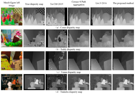
Figure 7.
Comparison of test image disparity maps obtained by different algorithms [16,18].
It can be seen from the figure that the reference [16] uses local block matching and does not go through the cost aggregation step. Therefore, although the matching time is fast, there are many missing and empty areas in the disparity map, and the matching effect is poor. The other three algorithms all use the cost aggregation strategy, and the processed disparity map has significantly fewer holes. Compared with the reference [18] method and the Census+8 path aggregation method, the method in this paper retains more complete information at the edge of the image and has less noise.
The matching effect of the proposed algorithm is evaluated by using the false matching rate. The false matching rate of the above four images is calculated in the non-occlusion (non), all (all), and disparity discontinuous (disc) regions. The average value is calculated, and the mismatch rate is obtained as shown in Table 3. The smaller the false matching rate, the smaller the gap between the results obtained by the method and the real disparity map, and the more accurate the matching results. As can be seen from the table, the four disparity maps obtained by the algorithm in this paper have a false matching rate of 6.88%, 7.61%, 5.85%, and 5.94%, and an average false matching rate of 6.57%, which are all lower than in the other three methods. Disparity maps are more accurate. As regards operation time, the running time of several algorithms is shown in Table 3. The algorithm in [16] does not use the path aggregation operation; therefore, the matching time is short, but relatively more disparity map noise leads to a high false matching rate. After the 4-path cost aggregation operation, the matching time is lengthened. The average running time of the Census+8 path aggregation algorithm is 21.86 s. The average running time of the algorithm in this paper is 5.68 s. The running time of the algorithm in this paper is longer than that of the reference [16] algorithm but much shorter than the Census+8 path aggregation algorithm and the reference [18] algorithm. It can be seen that the 4-path aggregation greatly shortens the running time of the algorithm. In summary, the matching accuracy of this paper is the highest among several methods, and the running time is faster. It can meet the real-time requirements. The effectiveness of the method proposed in this paper is verified.
Table 3.
Comparison table of disparity map evaluation indicators obtained by different algorithms.
- (2)
- Experiment 2
This experiment involves the stereo matching of sneaker sole images using an improved matching cost-based algorithm. The resulting disparity map looks as shown in Figure 8.
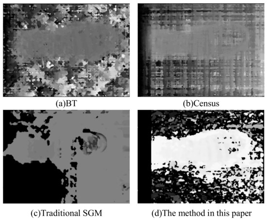
Figure 8.
Disparity map of shoe sole.
It can be seen from Figure 8 that the images obtained by other methods are blurred or missing. The contours of the disparity maps obtained by our method are clear and complete. The difference in parallax between the sole and its surroundings is well represented. The method in this paper shows a good stereo matching effect. The resulting 3D reconstruction renderings are shown below:
It can be seen from Figure 9 that the soles reconstructed based on the improved matching cost algorithm retain the details better. The traditional method is prone to the phenomenon of missing details. The point cloud has an obvious layering phenomenon, and the contours of the obtained toe and heel remain intact. There is still some noise due to background distractions. According to the difference between the color of the sole and the background, the obtained point cloud image is filtered to remove the black noise. The result obtained is shown in the Figure 10:

Figure 9.
3D reconstructed point cloud image of a shoe sole.
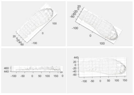
Figure 10.
The filtered point cloud image of a sneaker sole.
Due to the reflection phenomenon in some areas of the sole, the middle of the reconstructed sole is partially missing. But the edge information of the sole remains intact. This part of the information is also used for the extraction of the sole gluing trajectory. Therefore, the proposed method based on improved matching cost can meet the requirements. Experiments were carried out on the leather shoe sole shown i–n Figure 11. The effectiveness of the proposed method is further verified. The results are shown in Figure 12.
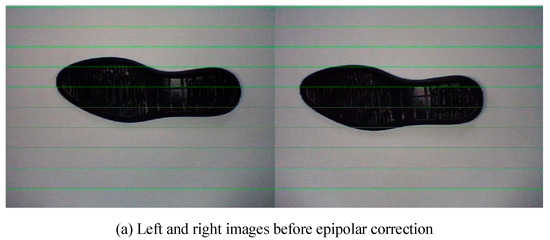
Figure 11.
Leather sole images before and after polar line correction.
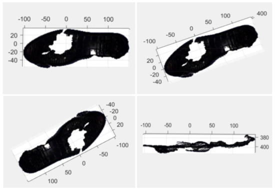
Figure 12.
The filtered point cloud image of leather shoe sole.
The reconstructed point cloud images of white sneaker soles and black leather shoe soles are observed. It is obtained that the 3D reconstruction of the sole can be better achieved based on the improved matching cost algorithm. The evaluation criteria of reference [12] were used. The maximum and minimum heights of the heel and toe center were measured. The height difference was calculated. The length data of the sole was obtained by calculating the distance between the heel and the center of the toe. The accuracy of the reconstructed point cloud was evaluated. The results are shown in the table below.
It can be seen from Table 4 that the error between the reconstructed sports shoe and the leather shoe sole is within 1.30mm. Its accuracy is relatively high, and there is no missing phenomenon in important positions such as the toe and heel. This method can meet the requirements of actual production.
Table 4.
Comparison table of reconstruction accuracy of different soles.
4. Conclusions
Due to rising labor cost, the quality requirements of shoe sole coating have gradually increased. Therefore, it is difficult for manual gluing to meet the needs of businesses. This paper adopts the method of fusing Census and BT cost to calculate the matching cost of left and right images. In this way, a more accurate matching cost can be obtained. At the same time, the 4-path aggregation strategy improves the efficiency of the algorithm. The parallax is optimized by using left–right consistency detection and median filtering methods. The proposed algorithm was evaluated with source images on the Middlebury website. The false matching rate was 6.57%, and the running speed was faster. In future research, it should be considered that when the number of feature points extracted is large, feature matching becomes difficult and there is an unnecessary matching burden. Non-maximum suppression can be cited to keep the point with the largest response and avoid the feature set. On the other hand, deep neural networks can learn more efficient features and metric functions to replace the cost computation of traditional stereo matching methods, thus improving the accuracy of stereo matching methods. At the same time, self-calibration methods [22,23] should be studied, as they have a wide range of usage environments and are flexible and adaptable.
Author Contributions
Conceptualization, R.W. and Z.G.; methodology, Z.G.; software, R.W.; validation, R.W., L.W., Z.G. and X.L.; formal analysis, R.W. and Z.G.; investigation, Z.G.; resources, L.W.; data curation, R.W.; writing—original draft preparation, R.W.; writing—review and editing, L.W.; visualization, Z.G.; supervision, L.W.; project administration, L.W.; funding acquisition, L.W. All authors have read and agreed to the published version of the manuscript.
Funding
This study was supported by The Natural Science Research Program of Colleges and Universities of Anhui Province under grant KJ2020ZD39, by the Open Research Fund of Anhui Key Laboratory of Detection Technology and Energy Saving Devices under grant DTESD2020A02, and by the Key Project of Graduate Teaching Reform and Research of Anhui Polytechnic University.
Data Availability Statement
Not applicable.
Conflicts of Interest
The authors declare no conflict of interest.
References
- Su, C.Y. In 2020, the global footwear industry production and trade both decline, and China’s production and sales still rank first. Beijing Leather 2021, 46, 74. [Google Scholar]
- Zhu, W.C. The future development trend of China’s shoe industry. Fujian Text. 2015, 5, 24. [Google Scholar]
- Ye, X.J. Challenges and opportunities coexist in China’s shoe industry. West Leather 2015, 13, 14–16. [Google Scholar]
- Ren, F.; Yu, X.; Dang, W.M. Depressive symptoms in Chinese assembly-line migrant workers: A case study in the shoe-making industry [J]. Asia-pacific psychiatry. Off. J. Pac. Rim Coll. Psychiatr. 2019, 11, 12332. [Google Scholar]
- Huang, G. Binocular vision system realizes real-time tracking of badminton. J. Electron. Meas. Instrum. 2021, 35, 117–123. [Google Scholar]
- Shi, L.; Zhu, H.H.; Yu, Y.; Cui, X.; Hui, L.; Chu, S.B.; Yang, L.; Zhang, S.K.; Zhou, Y. Research on wave parameter remote measurement method based on binocular stereo vision. J. Electron. Meas. Instrum. 2019, 33, 99–104. [Google Scholar]
- Chong, A.X.; Yin, H.; Liu, Y.T.; Liu, X.B.; Xu, H.L. Research on Longitudinal Displacement Measurement Method of Continuously Welded Rail Based on Binocular Vision. Chin. J. Sci. Instrum. 2019, 40, 82–89. [Google Scholar]
- Li, Z.Z.; Jiang, K.Y.; Lin, J.Y. Edge stereo matching algorithm of sole based on extreme constraint. Comput. Eng. Appl. 2016, 52, 217–220. [Google Scholar]
- Ding, D.K.; Shu, Y.F.; Xie, C.X. Application of Machine Vision in the Recognition of Motion Trajectory for Shoe Machine. Mach. Des. Manuf. 2018, 2, 257–259+262. [Google Scholar]
- Pagano, S.; Russo, R.; Savino, S. A vision guided robotic system for flexible gluing process in the footwear industry. Robot. Comput.-Integr. Manuf. 2020, 65, 101965. [Google Scholar] [CrossRef]
- Zhu, K.Y.; Wu, J.H. An Algorithm for Extracting Spray Trajectory Based on Laser Vision; Institute of Electrical and Electronics Engineers: Piscataway, NJ, USA, 2017; pp. 1591–1595. [Google Scholar]
- Ma, X.W.; Gan, Y. Research About Acquiring Sole Edge Information Based on Binocular Stereo Vision. Electron. Sci. Technol. 2017, 30, 58–62. [Google Scholar]
- Luo, J.F.; Qiu, G.; Zhang, Y.; Feng, S.; Han, L. Surf binocular vision matching algorithm based on adaptive dual thresh-old. Chin. J. Sci. Instrum. 2020, 41, 240–247. [Google Scholar]
- Yan, J.; Cao, Y.D.; Qu, Z. Stereo Matching Algorithm Based on Improved Census Transform. J. Liaoning Univ. Technol. (Nat. Sci. Ed.) 2021, 41, 11–14+37. [Google Scholar]
- Xiao, H.; Tian, C.; Zhang, Y.; Wei, B. Stereo matching algorithm based on improved Census transform and gradient fusion. Laser Optoelectron. Prog. 2021, 58, 327–333. [Google Scholar]
- Yu, C.H.; Zhang, J. Research on SAD-based stereo matching algorithm. J. Shenyang Inst. Aeronaut. Eng. 2019, 36, 77–83. [Google Scholar]
- Zhu, J.H.; Wang, C.S.; Gao, M.F. An improved matching algorithm of Census transform and adaptive window. Laser Optoelectron. Prog. 2021, 58, 427–434. [Google Scholar]
- Lin, J.; Kin, Y.; Lee, S. A Census transform-based robust stereo matching under radiometric changes. In Proceedings of the 2016 Asia-Pacific Signal and Information Processing Association Annual Summit and Conference, Jeju, Korea, 13–15 December 2016; pp. 1–4. [Google Scholar]
- Jia, K.B.; Du, Y.B. Stereo matching algorithm based on neighborhood information constraint and adaptive window. J. Beijing Univ. Technol. 2020, 46, 466–475. [Google Scholar]
- Jia, M.F.; Hu, G.Q.; Lu, C.Z. Research on automatic glue spray system based on image processing. Manuf. Autom. 2017, 39, 116–119. [Google Scholar]
- Sun, S. Research on Six-axis Robot Online Gluing System Based on Line Structured Light Vision Measuremen Technology; Anhui University of Technology: Ma’anshan, China, 2020. [Google Scholar]
- Hua, B.L.; Kai, W.W.; Kai, L.Y.; Rui, Q.C.; Chen, W.; Lei, F. Unconstrained self-calibration of stereo camera on visually impaired as-sistance devices. Appl. Opt. 2019, 58, 6377–6387. [Google Scholar]
- Bang, L.G.; Ying, J.Y.; Ang, S.; Yang, S.; Qi, F.Y. Self-calibration approach to stereo cameras with radial distortion based on epipolar constraint. Appl. Opt. 2019, 58, 8511–8521. [Google Scholar]
Publisher’s Note: MDPI stays neutral with regard to jurisdictional claims in published maps and institutional affiliations. |
© 2022 by the authors. Licensee MDPI, Basel, Switzerland. This article is an open access article distributed under the terms and conditions of the Creative Commons Attribution (CC BY) license (https://creativecommons.org/licenses/by/4.0/).