New Van der Pol–Duffing Jerk Fractional Differential Oscillator of Sequential Type

Abstract

The subject of this paper is the existence, uniqueness and stability of solutions for a new sequential Van der Pol–Duffing (VdPD) jerk fractional differential oscillator with Caputo–Hadamard derivatives. The arguments are based upon the Banach contraction principle, Krasnoselskii fixed-point theorem and Ulam–Hyers stabilities. As applications, one illustrative example is included to show the applicability of our results.

1. Introduction

Over the past four decades, the dynamical behaviors of nonlinear differential equations have been intensively studied by many researchers. This interest is justified by the promising applications generated by these equations; see, for example, refs. [1,2,3,4,5,6,7,8,9,10] and the references therein. Among the non-linear equations, the VdPD oscillator is a very prominent and interesting model that has been extensively studied in the context of several specific problems, such as chaos, control, synchronization, vibration description and asymptotic perturbation in physics, engineering, electronics, biology, neurology and many other disciplines; see, for instance, the research works [11,12,13,14,15,16,17,18].

The mathematical model for the VdPD oscillator is governed by a two-dimensional nonlinear differential equation of the form:

$$\frac{d^{2}u}{d{t}^2}-ϵ(1-u^2)\frac{du}{dt}+\alpha u-\beta u^3=fsin\left(\omega t\right),$$

(1)

where $\omega$ is the external frequency of the periodic signal and f stands for the amplitude of the external excitation. The parameters $ϵ$, $\alpha$ and $\beta$ are the dimensionless damping coefficient, linear and cubic nonlinearity parameters, respectively.

The authors in [19] proposed a three-dimensional problem for an autonomous VdPD oscillator obtained by a transformation of the autonomous two-dimensional VdPD oscillator into a jerk device with $f=0$ and $\alpha =1$ in the previous Equation (1), which they presented as follows:

$$\frac{d^{3}u}{d{t}^3}+\frac{d^{2}u}{d{t}^2}-ϵ(1-u^2)\frac{du}{dt}+u-\beta u^3=0,$$

(2)

where $ϵ$ and $\beta$ are positive parameters.

Recently, due to the frequent appearance of fractional derivatives in various applications in fluid mechanics, viscoelasticity, biology, physics and engineering, various kinds of VdPD jerk equations of fractional order have attracted more and more attention; see, for instance, refs. [19,20,21,22,23]. In this work, we try to propose an appropriate fractional formulation for a three-dimensional problem of the VdPD jerk type.

Therefore, let us consider the following problem:

$$\begin{array}{c}\hfill \left\{\begin{array}{c}{D}^{\alpha }(D^{2-\beta }+\lambda D^{\alpha })x\left(t\right)+k_1{f}_1(t,x\left(t\right),D^{\alpha }x\left(t\right))+k_2{f}_2(t,x\left(t\right),J^{p}x\left(t\right))=h\left(t\right).\\ \\ x\left(1\right)=0,D^{1-(\alpha -\beta )}{D}^{\alpha -\beta }x\left(1\right)=A^{*}\in \mathbb{R},x\left(T\right)=0,\\ \\ 0\le \beta <\alpha \le 1,0\le \alpha +\beta <1,0<p,t\in I,\end{array}\right.\end{array}$$

(3)

where $D^{\alpha },D^{2-\beta },$ are the Caputo–Hadamard fractional derivatives, $J^p$ is the Hadamard fractional integral $I=[1,T]$, $k_1,k_2$ are real constants, and the functions $f_1,f_2$ and h are continuous.

The motivation of our problem lies in using the Caputo–Hadamard approach in a sequential way, and the fact that this approach has many advantages over the usual Hadamard derivatives. Therefore, on the basis of these advantages, we have proposed the fractional problem associated with the (VdPL) jerk equation by injecting the Caputo–Hadamard derivatives on both sides of the equation with boundary conditions. This consideration makes the considered problem more interesting, knowing that when $\alpha =1$ and $\beta =0,$ we recover the type model (VdPL)-jerk.

The remaining part of this manuscript is distinguished as follows: in Section 2, we describe some basic notations of fractional derivatives and integrals and important results that will be used in subsequent parts of the paper. In Section 3, we prove three main theorems by applying the Banach contraction principle and Krasnoselskii fixed-point theorem. One of them concerns the Ulam–Hyers stability of Problem (3). Finally, Section 4 provides an example to illustrate the applicability of the main results.

2. Elementary Results

At first, we recall some concepts on fractional calculus and present some additional properties that will be used later. For more details, we refer to [24,25,26]. We present some basic definitions and results from fractional calculus theory.

Definition 1

(Hadamard fractional integral). The left-sided Hadamard fractional integral of order $\alpha \ge 0$, for a continuous function $f:[a,b]⟶\mathbb{R}$, is defined as

$$\begin{array}{cc}\hfill J_a^{\alpha }\left[f\left(t\right)\right]& =\frac{1}{\Gamma \left(\alpha \right)}{\int }_a^t{\left(logt-logs\right)}^{\alpha -1}f\left(s\right)\frac{ds}{s},\alpha >0,a<t\le b,\hfill \\ \hfill J_a^0\left[f\left(t\right)\right]& =f\left(t\right),\hfill \end{array}$$

where $\Gamma \left(\alpha \right):={\int }_0^{\infty }{e}^{-u}{u}^{\alpha -1}du$.

Definition 2

(Caputo–Hadamard fractional derivative). Let

$$A{C}_{\delta }^m\left([a,b]\right):=\left\{f:[a,b]⟶\mathbb{R}:{\delta }^{m-1}f\left(x\right)\in AC[a,b],\delta =t\frac{d}{dt}\right\}.$$

For a function $f\in A{C}_{\delta }^m\left([a,b]\right)$, $m\in {\mathbb{N}}^{*}$ and $m-1<\alpha \le m$, we define the Caputo–Hadamard fractional derivative by

$$\begin{array}{ccc}\hfill D^{\alpha }f\left(t\right)& =& \left\{\begin{array}{cc}\frac{1}{\Gamma (m-\alpha )}{\int }_a^t{\left(logt-logs\right)}^{m-\alpha -1}{\delta }^{m}f\left(s\right)\frac{ds}{s},\hfill & m-1<\alpha <m\hfill \\ \\ {\delta }^{m}f\left(t\right),\hfill & \alpha =m\hfill \end{array}\right.\hfill \\ & =& J^{m-\alpha }\left[{\delta }^{m}f\left(t\right)\right].\hfill \end{array}$$

Lemma 1.

Let $x\in A{C}_{\delta }^m\left([a,b]\right)$, $m\in {\mathbb{N}}^{*}$. The general solution of the equation

$$D^{\alpha }x\left(t\right)=0,$$

is given by

$$x\left(t\right)=c_0+c_{1}logt+c_2{(logt)}^2+...+c_{n-1}{(logt)}^{n-1},$$

and the following formula holds:

$$J^{\alpha }\left[D^{\alpha }x\left(t\right)\right]=x\left(t\right)+c_0+c_{1}logt+c_2{(logt)}^2+...+c_{n-1}{(logt)}^{n-1},$$

for some $c_i\in \mathbb{R},i=0,1,\cdots ,n-1,n=\left[\alpha \right]+1$.

Lemma 2.

Let $p,q>0$, $f\in L^1\left([a,b]\right)$. Then,

$$J^p{J}^q\left[f\left(t\right)\right]=J^{p+q}\left[f\left(t\right)\right],t\in [a,b].$$

Lemma 3.

Let $q>p>0$, $f\in L^1\left([a,b]\right)$. Then,

$$D^p{J}^q\left[f\left(t\right)\right]=J^{q-p}\left[f\left(t\right)\right],t\in [a,b].$$

Theorem 1

(Krasnoselskii fixed-point theorem). Let A be a closed convex and nonempty subset of a Banach space X, and let ${\varphi }_1$ and ${\varphi }_2$ be two operators such that

(${\mathfrak{U}}_1$)

${\varphi }_{1}x+{\varphi }_{2}y\in A$ whenever $x,y\in A$;

(${\mathfrak{U}}_2$)

${\varphi }_1$ is a completely continuous operator;

(${\mathfrak{U}}_3$)

${\varphi }_2$ is a contractive operator.

Then, there exists $x^{*}\in A,$ such that $x^{*}={\varphi }_1{x}^{*}+{\varphi }_2{x}^{*}$.

We prove also the following lemma:

Lemma 4.

Let $H\in C\left(\right[1,T\left]\right)$, $t\in I$, $0\le \beta <\alpha \le 1$. Then, the solution of the problem

$$\begin{array}{c}\hfill \left\{\begin{array}{c}{D}^{\alpha }(D^{2-\beta }+\lambda D^{\alpha })x\left(t\right)=H\left(t\right).\\ x\left(1\right)=0,D^{1-(\alpha -\beta )}{D}^{\alpha -\beta }x\left(1\right)=A^{*}\in \mathbb{R},x\left(T\right)=0,\end{array}\right.\end{array}$$

(4)

is given by the following expression:

$$\begin{array}{ccc}\hfill x\left(t\right)& =& \underset{1}{\overset{t}{\int }}\frac{{\left(logt-logs\right)}^{1-\beta +\alpha }}{\Gamma (2-\beta +\alpha )}H\left(s\right)\frac{ds}{s}-\lambda \underset{1}{\overset{t}{\int }}\frac{{\left(logt-logs\right)}^{1-(\alpha +\beta )}}{\Gamma (2-(\alpha +\beta \left)\right)}x\left(s\right)\frac{ds}{s}\hfill \\ & -& \left({\Lambda }_2{(logt)}^{2-\beta }+{\Lambda }_3{(logt)}^{2-(\alpha +\beta )}\right)\underset{1}{\overset{T}{\int }}\frac{{\left(logT-logs\right)}^{1-\beta +\alpha }}{\Gamma (2-\beta +\alpha )}H\left(s\right)\frac{ds}{s}\hfill \\ & +& \left({\Lambda }_2{(logt)}^{2-\beta }+{\Lambda }_3{(logt)}^{2-(\alpha +\beta )}\right)\lambda \underset{1}{\overset{T}{\int }}\frac{{\left(logT-logs\right)}^{1-(\alpha +\beta )}}{\Gamma (2-(\alpha +\beta \left)\right)}x\left(s\right)\frac{ds}{s}\hfill \\ & -& \left({\Lambda }_2{(logt)}^{2-\beta }+{\Lambda }_3{(logt)}^{2-(\alpha +\beta )}\right)\frac{A^{*}}{{\Lambda }_1}logT+A^{*}logt,\hfill \end{array}$$

(5)

where

$$\begin{array}{c}\hfill \begin{array}{ccccccc}{\Lambda }_1=\left(\frac{log{\left(T\right)}^{2-\beta }}{\Gamma (3-\beta )}+\frac{\lambda log{\left(T\right)}^{2-(\alpha +\beta )}}{\Gamma (3-(\alpha +\beta \left)\right)}\right)\hfill & & {\Lambda }_2=\frac{1}{{\Lambda }_1\Gamma (3-\beta )}\hfill & & & & {\Lambda }_3=\frac{\lambda }{{\Lambda }_1\Gamma (3-(\alpha +\beta ))}\hfill \end{array}.\end{array}$$

Proof. 

We apply Lemma 1, so the general solution of the Caputo–Hadamard fractional differential equation in (3) can be written as

$$\begin{array}{ccc}\hfill x\left(t\right)& =& J^{2-\beta +\alpha }H\left(t\right)-\lambda J^{2-(\alpha +\beta )}x\left(t\right)-\lambda c_0{J}^{2-(\alpha +\beta )}\left(1\right)-c_0{J}^{2-\beta }\left(1\right)-c_1-c_{2}logt,\hfill \end{array}$$

that is,

$$\begin{array}{ccc}\hfill x\left(t\right)& =& J^{2-\beta +\alpha }H\left(t\right)-\lambda J^{2-(\alpha +\beta )}x\left(t\right)-c_0\left(\frac{{(logt)}^{2-\beta }}{\Gamma (3-\beta )}+\frac{\lambda {(logt)}^{2-(\alpha +\beta )}}{\Gamma (3-(\alpha +\beta \left)\right)}\right)\hfill \\ & -& c_1-c_{2}logt,\hfill \end{array}$$

(6)

where $c_i\in \mathbb{R}$, $i=0,1,2$, are arbitrary real constants.

Using these conditions, we immediately obtain

$$\begin{array}{ccc}\hfill c_1& =& 0.\hfill \\ \hfill c_2& =& -A^{*}.\hfill \end{array}$$

On the other hand, we have

$$\begin{array}{ccc}\hfill c_0& =& \frac{1}{{\Lambda }_1}\left(J^{2-\beta +\alpha }H\left(T\right)-\lambda J^{2-(\alpha +\beta )}x\left(T\right)+A^{*}logT\right).\hfill \end{array}$$

Finally, inserting the values of $c_0,c_1$ and $c_2$ in (6), we obtain (5). The proof is completed. □

3. Main Results

This section is concerned with the main results of the paper.

First of all, we fix our terminology. Let X be the Banach space, defined as follows:

$$X:=\left\{x\in C(I,\mathbb{R}),D^{\alpha }x\in C(I,\mathbb{R})\right\},$$

endowed with the norm

$${\Vert x\Vert }_X={\Vert x\Vert }_{\infty }+{\Vert D^{\alpha }x\Vert }_{\infty },$$

where

$${\Vert x\Vert }_{\infty }=\underset{t\in I}{sup}\mid x\left(t\right)\mid ,{\Vert D^{\alpha }x\Vert }_{\infty }=\underset{t\in I}{sup}\mid D^{\alpha }x\left(t\right)\mid .$$

In view of Lemma 4, we introduce the operator $\varphi :X\to X$ as follows:

$$\begin{array}{ccc}\hfill \varphi x\left(t\right)& =& \underset{1}{\overset{t}{\int }}\frac{{\left(logt-logs\right)}^{1-\beta +\alpha }}{\Gamma (2-\beta +\alpha )}\left[\begin{array}{c}h\left(s\right)-k_1{f}_1(s,x\left(s\right),D^{\alpha }x\left(s\right))\hfill \\ -k_2{f}_2(s,x\left(s\right),J^{p}x\left(s\right))\hfill \end{array}\right]\frac{ds}{s}\hfill \\ & -& \lambda \underset{1}{\overset{t}{\int }}\frac{{\left(logt-logs\right)}^{1-(\alpha +\beta )}}{\Gamma (2-(\alpha +\beta \left)\right)}x\left(s\right)\frac{ds}{s}\hfill \\ & -& \left(\begin{array}{c}{\Lambda }_2{(logt)}^{2-\beta }\hfill \\ +{\Lambda }_3{(logt)}^{2-(\alpha +\beta )}\hfill \end{array}\right)\underset{1}{\overset{T}{\int }}\frac{{\left(logT-logs\right)}^{1-\beta +\alpha }}{\Gamma (2-\beta +\alpha )}\left[\begin{array}{c}h\left(s\right)\hfill \\ -k_1{f}_1(s,x\left(s\right),D^{\alpha }x\left(s\right))\hfill \\ -k_2{f}_2(s,x\left(s\right),J^{p}x\left(s\right))\hfill \end{array}\right]\frac{ds}{s}\hfill \\ & +& \left(\begin{array}{c}{\Lambda }_2{(logt)}^{2-\beta }\hfill \\ +{\Lambda }_3{(logt)}^{2-(\alpha +\beta )}\hfill \end{array}\right)\lambda \underset{1}{\overset{T}{\int }}\frac{{\left(logT-logs\right)}^{1-(\alpha +\beta )}}{\Gamma (2-(\alpha +\beta \left)\right)}x\left(s\right)\frac{ds}{s}\hfill \\ & -& \left({\Lambda }_2{(logt)}^{2-\beta }+{\Lambda }_3{(logt)}^{2-(\alpha +\beta )}\right)\frac{A^{*}}{{\Lambda }_1}logT+A^{*}logt.\hfill \end{array}$$

For computational convenience, we set the following quantities:

$$\begin{array}{ccc}\hfill N_1& =& \left(1+\left|{\Lambda }_2\right|{(logT)}^{2-\beta }+\left|{\Lambda }_3\right|{(logT)}^{2-(\alpha +\beta )}\right)\left[\begin{array}{c}\frac{(|k_1|L_1+|k_2|L_2){(logT)}^{2-\beta +\alpha }}{\Gamma (3-\beta +\alpha )}\hfill \\ \\ +\lambda \frac{{(logT)}^{2-(\alpha +\beta )}}{\Gamma (3-(\alpha +\beta \left)\right)}\hfill \end{array}\right].\hfill \\ \hfill N_2& =& \left[\begin{array}{c}\frac{(|k_1|L_1+|k_2|L_2){(logT)}^{2-\beta }}{\Gamma (3-\beta )}\hfill \\ +\frac{\lambda {(logT)}^{2-(2\alpha +\beta )}}{\Gamma (3-(2\alpha +\beta \left)\right)}\hfill \end{array}\right]+\left[\begin{array}{c}\frac{|{\Lambda }_2{|\Gamma (3-\beta )(logT)}^{2-(\alpha +\beta )}}{\Gamma (3-(\alpha +\beta \left)\right)}\hfill \\ +\frac{|{\Lambda }_3{|\Gamma (3-(\alpha +\beta ))(logT)}^{2-(2\alpha +\beta )}}{\Gamma (3-(2\alpha +\beta \left)\right)}\hfill \end{array}\right]\times \left[\begin{array}{c}\frac{|k_1|L_1{(logT)}^{2-\beta +\alpha }}{\Gamma (3-\beta +\alpha )}\hfill \\ +\frac{|k_2|L_2{(logT)}^{2-\beta +\alpha }}{\Gamma (3-\beta +\alpha )}\hfill \\ +\frac{\lambda {(logT)}^{2-(\alpha +\beta )}}{\Gamma (3-(\alpha +\beta \left)\right)}\hfill \end{array}\right].\hfill \\ \hfill N^{\prime }& =& \left\{\begin{array}{c}\frac{(|k_1|L_1+|k_2|L_2)\left(1+\left|{\Lambda }_2\right|{(logT)}^{2-\beta }+\left|{\Lambda }_3\right|{(logT)}^{2-(\alpha +\beta )}\right){(logT)}^{2-\beta +\alpha }}{\Gamma (3-\beta +\alpha )}\\ +(|k_1|L_1+|k_2|L_2)\left[\frac{{(logT)}^{2-\beta }}{\Gamma (3-\beta )}+\left(\begin{array}{c}\frac{|{\Lambda }_2{|\Gamma (3-\beta )(logT)}^{2-(\alpha +\beta )}}{\Gamma (3-(\alpha +\beta \left)\right)}\hfill \\ +\frac{|{\Lambda }_3{|\Gamma (3-(\alpha +\beta ))(logT)}^{2-(2\alpha +\beta )}}{\Gamma (3-(2\alpha +\beta \left)\right)}\hfill \end{array}\right)\frac{{(logT)}^{2-\beta +\alpha }}{\Gamma (3-\beta +\alpha )}\right].\end{array}\right.\hfill \end{array}$$

Then, we take into account the following hypothesis:

(H1):

There exist non-negative constants $L_1,L_2$, such that for each $t\in I$ and for all

$(x_1,y_1),(x_2,y_2)\in {\mathbb{R}}^2$, we have:

$$\begin{array}{ccc}\hfill |f_1(t,x_1,y_1)-f_1(t,x_2,y_2))|& \le & L_1(|x_1-x_2|+|y_1-y_2|).\hfill \\ \hfill |f_2(t,x_1,y_1)-f_2(t,x_2,y_2))|& \le & L_2(|x_1-x_2|+|y_1-y_2|).\hfill \end{array}$$

(H2):

The functions $f_1:I\times {\mathbb{R}}^2\to \mathbb{R}$, $f_2:I\times {\mathbb{R}}^2\to \mathbb{R}$ are continuous.

(H3):

There exists non-negative constants $E_1,E_2$ and $E_3$, such that for each $t\in I$ and all $x_1,x_2\in \mathbb{R}$, we have:

$$\begin{array}{c}\hfill \begin{array}{ccc}|f_1(t,x_1,x_2))|\le E_1,& |f_2(t,x_1,x_2)|\le E_2,& |h\left(t\right)|\le E_3.\end{array}\end{array}$$

3.1. An Existence and Uniqueness Result in Banach Space

In this section, fixed-point theorems are applied to present an existence and uniqueness result concerning Problem (3). First, the Banach contraction principle is applied to establish the uniqueness result.

Theorem 2.

Assume that (H1) and (H2) are valid. Assume also that

$$0<N<1,$$

(7)

where $N:=N_1+N_2$.

Then, the problem (3) has a unique solution on I.

Proof. 

We shall show that the above application $\varphi$ is contractive. Therefore, we need to proceed in steps A and B:

Step A: Let $x,y\in X$; we then have:

$$\begin{array}{c}\hfill |\varphi x(t)-\varphi y(t)|\\ \hfill \le & \underset{t\in I}{sup}\underset{1}{\overset{t}{\int }}\frac{{\left(logt-logs\right)}^{1-\beta +\alpha }}{\Gamma (2-\beta +\alpha )}|k_1||f_1(s,x\left(s\right),D^{\alpha }x\left(s\right))-f_1(s,y\left(s\right),D^{\alpha }y\left(s\right))|\frac{ds}{s}\\ \hfill +& \underset{t\in I}{sup}\left(\begin{array}{c}\left|{\Lambda }_2{(logt)}^{2-\beta }\right|\hfill \\ +\left|{\Lambda }_3{(logt)}^{2-(\alpha +\beta )}\right|\hfill \end{array}\right)\underset{1}{\overset{T}{\int }}\frac{{\left(logT-logs\right)}^{1-\beta +\alpha }}{\Gamma (2-\beta +\alpha )}|k_1|\left|\begin{array}{c}{f}_1(s,x\left(s\right),D^{\alpha }x\left(s\right))\hfill \\ -f_1(s,y\left(s\right),D^{\alpha }y\left(s\right))\hfill \end{array}\right|\frac{ds}{s}\\ \hfill +& \underset{t\in I}{sup}\underset{1}{\overset{t}{\int }}\frac{{\left(logt-logs\right)}^{1-\beta +\alpha }}{\Gamma (2-\beta +\alpha )}|k_2||f_2(s,x\left(s\right),J^{p}x\left(s\right))-f_2(s,y\left(s\right),J^{p}y\left(s\right))|\frac{ds}{s}\\ \hfill +& \underset{t\in I}{sup}\left(\begin{array}{c}\left|{\Lambda }_2{(logt)}^{2-\beta }\right|\hfill \\ +\left|{\Lambda }_3{(logt)}^{2-(\alpha +\beta )}\right|\hfill \end{array}\right)\underset{1}{\overset{T}{\int }}\frac{{\left(logT-logs\right)}^{1-\beta +\alpha }}{\Gamma (2-\beta +\alpha )}|k_2|\left|\begin{array}{c}{f}_2(s,x\left(s\right),J^{p}x\left(s\right))\hfill \\ -f_2(s,y\left(s\right),J^{p}y\left(s\right))\hfill \end{array}\right|\frac{ds}{s}\\ \hfill +& \underset{t\in I}{sup}\lambda \underset{1}{\overset{t}{\int }}\frac{{\left(logt-logs\right)}^{1-(\alpha +\beta )}}{\Gamma (2-(\alpha +\beta \left)\right)}|x\left(s\right)-y\left(s\right)|\frac{ds}{s}\\ \hfill +& \underset{t\in I}{sup}\left(\left|{\Lambda }_2{(logt)}^{2-\beta }\right|+\left|{\Lambda }_3{(logt)}^{2-(\alpha +\beta )}\right|\right)\lambda \underset{1}{\overset{T}{\int }}\frac{{\left(logT-logs\right)}^{1-(\alpha +\beta )}}{\Gamma (2-(\alpha +\beta \left)\right)}|x\left(s\right)-y\left(s\right)|\frac{ds}{s}.\end{array}$$

By assumption (H1), we obtain:

$$\begin{array}{ccc}\hfill |\varphi x(t)-\varphi y(t)|& \le & |k_1|L_1{(\Vert x-y\Vert }_{\infty }+\Vert D^{\alpha }x-D^{\alpha }y{\Vert }_{\infty })\frac{{(logT)}^{2-\beta +\alpha }}{\Gamma (3-\beta +\alpha )}\hfill \\ & +& |k_1|L_1\left(\begin{array}{c}\left|{\Lambda }_2\right|{(logT)}^{2-\beta }\hfill \\ +\left|{\Lambda }_3\right|{(logT)}^{2-(\alpha +\beta )}\hfill \end{array}\right)\left(\begin{array}{c}{\Vert x-y\Vert }_{\infty }\hfill \\ +\Vert D^{\alpha }x-D^{\alpha }{y\Vert }_{\infty }\hfill \end{array}\right)\frac{{(logT)}^{2-\beta +\alpha }}{\Gamma (3-\beta +\alpha )}\hfill \\ & +& |k_2|L_2{(\Vert x-y\Vert }_{\infty }+\Vert J^{p}x-J^{p}y{\Vert }_{\infty })\frac{{(logT)}^{2-\beta +\alpha }}{\Gamma (3-\beta +\alpha )}\hfill \\ & +& |k_2|L_2\left(\begin{array}{c}\left|{\Lambda }_2\right|{(logT)}^{2-\beta }\hfill \\ +\left|{\Lambda }_3\right|{(logT)}^{2-(\alpha +\beta )}\hfill \end{array}\right)\left(\begin{array}{c}{\Vert x-y\Vert }_{\infty }\hfill \\ +\Vert J^{p}x-J^p{y\Vert }_{\infty }\hfill \end{array}\right)\frac{{(logT)}^{2-\beta +\alpha }}{\Gamma (3-\beta +\alpha )}\hfill \\ & +& {\lambda \Vert x-y\Vert }_{\infty }\frac{{(logT)}^{2-(\alpha +\beta )}}{\Gamma (3-(\alpha +\beta \left)\right)}\hfill \\ & +& \lambda \left(\left|{\Lambda }_2\right|{(logT)}^{2-\beta }+\left|{\Lambda }_3\right|{(logT)}^{2-(\alpha +\beta )}\right){\Vert x-y\Vert }_{\infty }\frac{{(logT)}^{2-(\alpha +\beta )}}{\Gamma (3-(\alpha +\beta \left)\right)}.\hfill \end{array}$$

Consequently, the inequality holds:

$$\begin{array}{ccc}\hfill {\Vert \varphi x-\varphi y\Vert }_{\infty }& \le & |k_1|L_1{\Vert x-y\Vert }_X\frac{{(logT)}^{2-\beta +\alpha }}{\Gamma (3-\beta +\alpha )}\hfill \\ & +& |k_1|L_1\left(\left|{\Lambda }_2\right|{(logT)}^{2-\beta }+\left|{\Lambda }_3\right|{(logT)}^{2-(\alpha +\beta )}\right){\Vert x-y\Vert }_X\frac{{(logT)}^{2-\beta +\alpha }}{\Gamma (3-\beta +\alpha )}\hfill \\ & +& |k_2|L_2{\Vert x-y\Vert }_X\frac{{(logT)}^{2-\beta +\alpha }}{\Gamma (3-\beta +\alpha )}\hfill \\ & +& |k_2|L_2\left(\left|{\Lambda }_2\right|{(logT)}^{2-\beta }+\left|{\Lambda }_3\right|{(logT)}^{2-(\alpha +\beta )}\right){\Vert x-y\Vert }_X\frac{{(logT)}^{2-\beta +\alpha }}{\Gamma (3-\beta +\alpha )}\hfill \\ & +& {\lambda \Vert x-y\Vert }_X\frac{{(logT)}^{2-(\alpha +\beta )}}{\Gamma (3-(\alpha +\beta \left)\right)}\hfill \\ & +& \lambda \left(\left|{\Lambda }_2\right|{(logT)}^{2-\beta }+\left|{\Lambda }_3\right|{(logT)}^{2-(\alpha +\beta )}\right){\Vert x-y\Vert }_X\frac{{(logT)}^{2-(\alpha +\beta )}}{\Gamma (3-(\alpha +\beta \left)\right)}.\hfill \\ & \le & \left[\begin{array}{c}\frac{(|k_1|L_1+|k_2|L_2)\left(1+\left|{\Lambda }_2\right|{(logT)}^{2-\beta }+\left|{\Lambda }_3\right|{(logT)}^{2-(\alpha +\beta )}\right){(logT)}^{2-\beta +\alpha }}{\Gamma (3-\beta +\alpha )}\hfill \\ \\ +\lambda \frac{\left(1+\left|{\Lambda }_2\right|{(logT)}^{2-\beta }+\left|{\Lambda }_3\right|{(logT)}^{2-(\alpha +\beta )}\right){(logT)}^{2-(\alpha +\beta )}}{\Gamma (3-(\alpha +\beta \left)\right)}\hfill \end{array}\right]{\Vert x-y\Vert }_X\hfill \\ & \le & \left(\begin{array}{c}1+\left|{\Lambda }_2\right|{(logT)}^{2-\beta }\hfill \\ +\left|{\Lambda }_3\right|{(logT)}^{2-(\alpha +\beta )}\hfill \end{array}\right)\left[\begin{array}{c}\frac{(|k_1|L_1+|k_2|L_2){(logT)}^{2-\beta +\alpha }}{\Gamma (3-\beta +\alpha )}\hfill \\ \\ +\lambda \frac{{(logT)}^{2-(\alpha +\beta )}}{\Gamma (3-(\alpha +\beta \left)\right)}\hfill \end{array}\right]{\Vert x-y\Vert }_X.\hfill \end{array}$$

Therefore,

$$\begin{array}{ccc}\hfill {\Vert \varphi x-\varphi y\Vert }_{\infty }& \le & N_1{\Vert x-y\Vert }_X.\hfill \end{array}$$

Step B: Let $x,y\in X$, we have:

$$\begin{array}{ccc}\hfill D^{\alpha }\varphi x\left(t\right)& =& \underset{1}{\overset{t}{\int }}\frac{{\left(logt-logs\right)}^{1-\beta }}{\Gamma (2-\beta )}\left[\begin{array}{c}h\left(s\right)-k_1{f}_1(s,x\left(s\right),D^{\alpha }x\left(s\right))\hfill \\ -k_2{f}_2(s,x\left(s\right),J^{p}x\left(s\right))\hfill \end{array}\right]\frac{ds}{s}\hfill \\ & -& \lambda \underset{1}{\overset{t}{\int }}\frac{{\left(logt-logs\right)}^{2-(2\alpha +\beta )-1}}{\Gamma (2-(2\alpha +\beta \left)\right)}x\left(s\right)\frac{ds}{s}+\frac{A^{*}{(logt)}^{1-\alpha }}{\Gamma (2-\alpha )}\hfill \\ & -& \frac{{\Lambda }_2\Gamma (3-\beta ){(logt)}^{2-(\alpha +\beta )}}{\Gamma (3-(\alpha +\beta \left)\right)}\underset{1}{\overset{T}{\int }}\frac{{\left(logT-logs\right)}^{1-\beta +\alpha }}{\Gamma (2-\beta +\alpha )}\left[\begin{array}{c}h\left(s\right)\hfill \\ -k_1{f}_1(s,x\left(s\right),D^{\alpha }x\left(s\right))\hfill \\ -k_2{f}_2(s,x\left(s\right),J^{p}x\left(s\right))\hfill \end{array}\right]\frac{ds}{s}\hfill \\ & -& \frac{{\Lambda }_3\Gamma (3-(\alpha +\beta )){(logt)}^{2-(2\alpha +\beta )}}{\Gamma (3-(2\alpha +\beta \left)\right)}\underset{1}{\overset{T}{\int }}\frac{{\left(logT-logs\right)}^{1-\beta +\alpha }}{\Gamma (2-\beta +\alpha )}\left[\begin{array}{c}h\left(s\right)\hfill \\ -k_1{f}_1(s,x\left(s\right),D^{\alpha }x\left(s\right))\hfill \\ -k_2{f}_2(s,x\left(s\right),J^{p}x\left(s\right))\hfill \end{array}\right]\frac{ds}{s}\hfill \\ & +& \lambda \frac{{\Lambda }_2\Gamma (3-\beta ){(logt)}^{2-(\alpha +\beta )}}{\Gamma (3-(\alpha +\beta \left)\right)}\underset{1}{\overset{T}{\int }}\frac{{\left(logT-logs\right)}^{1-(\alpha +\beta )}}{\Gamma (2-(\alpha +\beta \left)\right)}x\left(s\right)\frac{ds}{s}\hfill \\ & +& \lambda \frac{{\Lambda }_3\Gamma (3-(\alpha +\beta )){(logt)}^{2-(2\alpha +\beta )}}{\Gamma (3-(2\alpha +\beta \left)\right)}\underset{1}{\overset{T}{\int }}\frac{{\left(logT-logs\right)}^{1-(\alpha +\beta )}}{\Gamma (2-(\alpha +\beta \left)\right)}x\left(s\right)\frac{ds}{s}\hfill \\ & -& \frac{A^{*}{\Lambda }_2\Gamma (3-\beta ){(logt)}^{2-(\alpha +\beta )}}{{\Lambda }_1\Gamma (3-(\alpha +\beta ))}logT-\frac{A^{*}{\Lambda }_3\Gamma (3-(\alpha +\beta )){(logt)}^{2-(2\alpha +\beta )}}{{\Lambda }_1\Gamma (3-(2\alpha +\beta ))}logT.\hfill \end{array}$$

Then,

$$\begin{array}{ccc}\hfill \Vert D^{\alpha }\varphi x-D^{\alpha }{\varphi y\Vert }_{\infty }& \le & \frac{(|k_1|L_1+|k_2|L_2){(logT)}^{2-\beta }}{\Gamma (3-\beta )}{\Vert x-y\Vert }_X+\lambda \frac{{(logT)}^{2-(2\alpha +\beta )}}{\Gamma (3-(2\alpha +\beta \left)\right)}{\Vert x-y\Vert }_X\hfill \\ & +& \left(\begin{array}{c}|k_1|L_1\hfill \\ +|k_2|L_2\hfill \end{array}\right)\left[\begin{array}{c}\frac{|{\Lambda }_2{|\Gamma (3-\beta )(logT)}^{2-(\alpha +\beta )}}{\Gamma (3-(\alpha +\beta \left)\right)}\hfill \\ +\frac{|{\Lambda }_3{|\Gamma (3-(\alpha +\beta ))(logT)}^{2-(2\alpha +\beta )}}{\Gamma (3-(2\alpha +\beta \left)\right)}\hfill \end{array}\right]\frac{{(logT)}^{2-\beta +\alpha }}{\Gamma (3-\beta +\alpha )}{\Vert x-y\Vert }_X\hfill \\ & +& \lambda \left[\begin{array}{c}\frac{|{\Lambda }_2{|\Gamma (3-\beta )(logT)}^{2-(\alpha +\beta )}}{\Gamma (3-(\alpha +\beta \left)\right)}\hfill \\ +\frac{|{\Lambda }_3{|\Gamma (3-(\alpha +\beta ))(logT)}^{2-(2\alpha +\beta )}}{\Gamma (3-(2\alpha +\beta \left)\right)}\hfill \end{array}\right]\frac{{(logT)}^{2-(\alpha +\beta )}}{\Gamma (3-(\alpha +\beta \left)\right)}{\Vert x-y\Vert }_X\hfill \\ & \le & N_2{\Vert x-y\Vert }_X.\hfill \end{array}$$

Thus,

$$\begin{array}{ccc}\hfill \Vert D^{\alpha }\varphi x-D^{\alpha }{\varphi y\Vert }_{\infty }& \le & \left[\frac{(|k_1|L_1+|k_2|L_2){(logT)}^{2-\beta }}{\Gamma (3-\beta )}+\frac{\lambda {(logT)}^{2-(2\alpha +\beta )}}{\Gamma (3-(2\alpha +\beta \left)\right)}\right]{\Vert x-y\Vert }_X\hfill \\ & +& \left[\begin{array}{c}\frac{|{\Lambda }_2{|\Gamma (3-\beta )(logT)}^{2-(\alpha +\beta )}}{\Gamma (3-(\alpha +\beta \left)\right)}\hfill \\ +\frac{|{\Lambda }_3{|\Gamma (3-(\alpha +\beta ))(logT)}^{2-(2\alpha +\beta )}}{\Gamma (3-(2\alpha +\beta \left)\right)}\hfill \end{array}\right]\times \left[\begin{array}{c}\frac{|k_1|L_1{(logT)}^{2-\beta +\alpha }}{\Gamma (3-\beta +\alpha )}\hfill \\ +\frac{|k_2|L_2{(logT)}^{2-\beta +\alpha }}{\Gamma (3-\beta +\alpha )}\hfill \\ +\frac{\lambda {(logT)}^{2-(\alpha +\beta )}}{\Gamma (3-(\alpha +\beta \left)\right)}\hfill \end{array}\right]{\Vert x-y\Vert }_X\hfill \\ & \le & N_2{\Vert x-y\Vert }_X.\hfill \end{array}$$

Therefore, the final result is given by:

$$\begin{array}{c}\hfill {\Vert \varphi x-\varphi y\Vert }_X\le N{\Vert x-y\Vert }_X.\end{array}$$

Consequently, by (7), $\varphi$ is a contraction, and by applying Banach’s fixed point theorem, Problem (3) has a unique solution. The proof is completed. □

Now, by applying the Krasnoselskii fixed-point theorem, we prove an existence result for Problem (3).

Theorem 3.

Assume that the hypotheses (H2) and (H3) are satisfied. Then, Problem (3) has at least a solution on I, provided that $0<N^{\prime }<1$.

Proof. 

We verify that the assumptions of a Krasnoselskii fixed-point (Theorem 1) are satisfied by the operator $\varphi$.

First of all, we introduce the convex closed subspace ${\mathfrak{B}}_{\mathfrak{r}}\in X$ defined by:

$${\mathfrak{B}}_{\mathfrak{r}}:=\left\{x\in {X:\parallel x\parallel }_X\le r\right\}$$

Then, we split the operator $\varphi$ into the sum of two operators, ${\varphi }_1$ and ${\varphi }_2$, on the closed ball ${\mathfrak{B}}_{\mathfrak{r}}$ as:

$$\begin{array}{ccc}\hfill {\varphi }_{1}x\left(t\right)& =& -\lambda \underset{1}{\overset{t}{\int }}\frac{{\left(logt-logs\right)}^{1-(\alpha +\beta )}}{\Gamma (2-(\alpha +\beta \left)\right)}x\left(s\right)\frac{ds}{s}\hfill \\ & +& \left({\Lambda }_2{(logt)}^{2-\beta }+{\Lambda }_3{(logt)}^{2-(\alpha +\beta )}\right)\lambda \underset{1}{\overset{T}{\int }}\frac{{\left(logT-logs\right)}^{1-(\alpha +\beta )}}{\Gamma (2-(\alpha +\beta \left)\right)}x\left(s\right)\frac{ds}{s},\hfill \end{array}$$

and

$$\begin{array}{ccc}\hfill {\varphi }_{2}x\left(t\right)& =& \underset{1}{\overset{t}{\int }}\frac{{\left(logt-logs\right)}^{1-\beta +\alpha }}{\Gamma (2-\beta +\alpha )}\left[\begin{array}{c}h\left(s\right)-k_1{f}_1(s,x\left(s\right),D^{\alpha }x\left(s\right))\hfill \\ -k_2{f}_2(s,x\left(s\right),J^{p}x\left(s\right))\hfill \end{array}\right]\frac{ds}{s}\hfill \\ & -& \left(\begin{array}{c}{\Lambda }_2{(logt)}^{2-\beta }\hfill \\ +{\Lambda }_3{(logt)}^{2-(\alpha +\beta )}\hfill \end{array}\right)\underset{1}{\overset{T}{\int }}\frac{{\left(logT-logs\right)}^{1-\beta +\alpha }}{\Gamma (2-\beta +\alpha )}\left[\begin{array}{c}h\left(s\right)\hfill \\ -k_1{f}_1(s,x\left(s\right),D^{\alpha }x\left(s\right))\hfill \\ -k_2{f}_2(s,x\left(s\right),J^{p}x\left(s\right))\hfill \end{array}\right]\frac{ds}{s}\hfill \\ \hfill \\ & -& \left({\Lambda }_2{(logt)}^{2-\beta }+{\Lambda }_3{(logt)}^{2-(\alpha +\beta )}\right)\frac{A^{*}}{{\Lambda }_1}logT+A^{*}logt.\hfill \end{array}$$

The proof is divided into three steps.

First, we show that ${\varphi }_{1}x+{\varphi }_{2}y\in {\mathfrak{B}}_{\mathfrak{r}}$, $\forall x,y\in {\mathfrak{B}}_{\mathfrak{r}}$. Then, we prove that the operator ${\varphi }_2$ is a contraction on ${\mathfrak{B}}_{\mathfrak{r}}$. Finally, we show that ${\varphi }_1$ is a compact operator.

1: 

For $x,y\in {\mathfrak{B}}_{\mathfrak{r}}$, $t\in I$, we can write:

$$\begin{array}{c}\hfill |{\varphi }_{1}x\left(t\right)+{\varphi }_{2}y\left(t\right)|\\ \hfill \le & \underset{t\in I}{sup}\left|\underset{1}{\overset{t}{\int }}\frac{{\left(logt-logs\right)}^{1-\beta +\alpha }}{\Gamma (2-\beta +\alpha )}\right.\left[\begin{array}{c}h\left(s\right)\hfill \\ -k_1{f}_1(s,y\left(s\right),D^{\alpha }y\left(s\right))\hfill \\ -k_2{f}_2(s,y\left(s\right),J^{p}y\left(s\right))\hfill \end{array}\right]\frac{ds}{s}\\ \hfill -& \left(\begin{array}{c}{\Lambda }_2{(logt)}^{2-\beta }\hfill \\ +{\Lambda }_3{(logt)}^{2-(\alpha +\beta )}\hfill \end{array}\right)\underset{1}{\overset{T}{\int }}\frac{{\left(logT-logs\right)}^{1-\beta +\alpha }}{\Gamma (2-\beta +\alpha )}\left[\begin{array}{c}h\left(s\right)\hfill \\ -k_1{f}_1(s,y\left(s\right),D^{\alpha }y\left(s\right))\hfill \\ -k_2{f}_2(s,y\left(s\right),J^{p}y\left(s\right))\hfill \end{array}\right]\frac{ds}{s}\\ \hfill +& \left(\begin{array}{c}{\Lambda }_2{(logt)}^{2-\beta }\hfill \\ +{\Lambda }_3{(logt)}^{2-(\alpha +\beta )}\hfill \end{array}\right)\lambda \underset{1}{\overset{T}{\int }}\frac{{\left(logT-logs\right)}^{1-(\alpha +\beta )}}{\Gamma (2-(\alpha +\beta \left)\right)}x\left(s\right)\frac{ds}{s}\\ \hfill -& \lambda \underset{1}{\overset{t}{\int }}\frac{{\left(logt-logs\right)}^{1-(\alpha +\beta )}}{\Gamma (2-(\alpha +\beta \left)\right)}x\left(s\right)\frac{ds}{s}-\left.\left(\begin{array}{c}{\Lambda }_2{(logt)}^{2-\beta }\hfill \\ +{\Lambda }_3{(logt)}^{2-(\alpha +\beta )}\hfill \end{array}\right)\frac{A^{*}}{{\Lambda }_1}logT+A^{*}logt\right|.\end{array}$$

By (H3), we have:

$$\begin{array}{ccc}\hfill \parallel {\varphi }_{1}x+{\varphi }_2{y\parallel }_{\infty }& \le & \left(1+S_1\right))\times \left[\begin{array}{c}\frac{(E_h+|k_1|E_{f_1}+|k_2|E_{f_2}){(logT)}^{2-\beta +\alpha }}{\Gamma (3-\beta +\alpha )}\hfill \\ +\frac{\lambda r{(logT)}^{2-(\alpha +\beta )}}{\Gamma (3-(\alpha +\beta \left)\right)}\hfill \end{array}\right]+|A^{*}|logT\left(\frac{S_1}{|{\Lambda }_1|}+1\right)\hfill \\ & \le & \left(1+S_1\right))\times \left[\begin{array}{c}\frac{(E_h+|k_1|E_{f_1}+|k_2|E_{f_2}){(logT)}^{2-\beta +\alpha }}{\Gamma (3-\beta +\alpha )}\hfill \\ +\frac{\lambda r{(logT)}^{2-(\alpha +\beta )}}{\Gamma (3-(\alpha +\beta \left)\right)}\hfill \end{array}\right]+C_1,\hfill \end{array}$$

where $S_1=|{\Lambda }_2{|(logT)}^{2-\beta }+|{\Lambda }_3|{(logT)}^{2-(\alpha +\beta )}$.

Then, we have:

$$\begin{array}{ccc}\hfill \parallel D^{\alpha }\varphi x+D^{\alpha }{\varphi y\parallel }_{\infty }& \le & (E_h+|k_1|E_{f_1}+|k_2|E_{f_2})\left[\frac{{(logT)}^{2-\beta }}{\Gamma (3-\beta )}+S_2\frac{{(logT)}^{2-\beta +\alpha }}{\Gamma (3-\beta +\alpha )}\right]\hfill \\ & +& \lambda r\left[\frac{{(logT)}^{2-(2\alpha +\beta )}}{\Gamma (3-(2\alpha +\beta \left)\right)}+S_2\frac{{(logT)}^{2-(\alpha +\beta )}}{\Gamma (3-(\alpha +\beta \left)\right)}\right]\hfill \\ & +& |A^{*}|\left[\frac{{(logT)}^{1-\alpha }}{\Gamma (2-\alpha )}+S_{2}logT\right]\hfill \\ & \le & (E_h+|k_1|E_{f_1}+|k_2|E_{f_2})\left[\frac{{(logT)}^{2-\beta }}{\Gamma (3-\beta )}+S_2\frac{{(logT)}^{2-\beta +\alpha }}{\Gamma (3-\beta +\alpha )}\right]\hfill \\ & +& \lambda r\left[\frac{{(logT)}^{2-(2\alpha +\beta )}}{\Gamma (3-(2\alpha +\beta \left)\right)}+S_2\frac{{(logT)}^{2-(\alpha +\beta )}}{\Gamma (3-(\alpha +\beta \left)\right)}\right]+C_2,\hfill \end{array}$$

where $S_2=|{\Lambda }_2|\frac{\Gamma (3-\beta ){(logT)}^{2-(\alpha +\beta )}}{\Gamma (3-(\alpha +\beta \left)\right)}+|{\Lambda }_3|\frac{\Gamma (3-(\alpha +\beta )){(logT)}^{2-(2\alpha +\beta )}}{\Gamma (3-(2\alpha +\beta \left)\right)}$.

We put

$$\begin{array}{ccc}\hfill r& =& \left\{\begin{array}{c}\left(1+S_1\right))\times \left[\begin{array}{c}\frac{(E_h+|k_1|E_{f_1}+|k_2|E_{f_2}){(logT)}^{2-\beta +\alpha }}{\Gamma (3-\beta +\alpha )}\hfill \\ +\frac{\lambda r{(logT)}^{2-(\alpha +\beta )}}{\Gamma (3-(\alpha +\beta \left)\right)}\hfill \end{array}\right]+C_1\\ \\ +(E_h+|k_1|E_{f_1}+|k_2|E_{f_2})\left[\frac{{(logT)}^{2-\beta }}{\Gamma (3-\beta )}+S_2\frac{{(logT)}^{2-\beta +\alpha }}{\Gamma (3-\beta +\alpha )}\right]\\ +\lambda r\left[\frac{{(logT)}^{2-(2\alpha +\beta )}}{\Gamma (3-(2\alpha +\beta \left)\right)}+S_2\frac{{(logT)}^{2-(\alpha +\beta )}}{\Gamma (3-(\alpha +\beta \left)\right)}\right]+C_2.\end{array}\right.\hfill \end{array}$$

Then, we deduce that

$${\parallel \varphi x+\varphi y\parallel }_X\le r.$$

This implies that ${\varphi }_{1}x+{\varphi }_{2}y\in {\mathfrak{B}}_{\mathfrak{r}}$ , $\forall x,y\in {\mathfrak{B}}_{\mathfrak{r}}$.

2: 

We will show that ${\varphi }_2$ is a contraction on ${\mathfrak{B}}_{\mathfrak{r}}.$ Let $x,y\in {\mathfrak{B}}_{\mathfrak{r}},$ with $t\in I$. We have

$$\begin{array}{ccc}\hfill \Vert {\varphi }_{2}x-{\varphi }_2{y\Vert }_{\infty }& \le & \frac{(|k_1|L_1+|k_2|L_2)\left(\begin{array}{c}1+\left|{\Lambda }_2\right|{(logT)}^{2-\beta }\hfill \\ +\left|{\Lambda }_3\right|{(logT)}^{2-(\alpha +\beta )}\hfill \end{array}\right){(logT)}^{2-\beta +\alpha }}{\Gamma (3-\beta +\alpha )}{\Vert x-y\Vert }_X.\hfill \end{array}$$

On the other hand, we have:

$$\begin{array}{ccc}\hfill \Vert D^{\alpha }{\varphi }_{2}x-D^{\alpha }{\varphi }_2{y\Vert }_{\infty }& \le & \left(\begin{array}{c}|k_1|L_1\hfill \\ +|k_2|L_2\hfill \end{array}\right)\left[\begin{array}{c}\frac{{(logT)}^{2-\beta }}{\Gamma (3-\beta )}\hfill \\ +\left(\begin{array}{c}\frac{|{\Lambda }_2{|\Gamma (3-\beta )(logT)}^{2-(\alpha +\beta )}}{\Gamma (3-(\alpha +\beta \left)\right)}\hfill \\ +\frac{|{\Lambda }_3{|\Gamma (3-(\alpha +\beta ))(logT)}^{2-(2\alpha +\beta )}}{\Gamma (3-(2\alpha +\beta \left)\right)}\hfill \end{array}\right)\hfill \\ \times \frac{{(logT)}^{2-\beta +\alpha }}{\Gamma (3-\beta +\alpha )}\hfill \end{array}\right]{\Vert x-y\Vert }_X.\hfill \end{array}$$

Therefore, it yields that

$$\Vert {\varphi }_{2}x-{\varphi }_2{y\Vert }_X\le N^{{}^{\prime }}{\Vert x-y\Vert }_X.$$

3: 

We show that ${\varphi }_1$ is a compact operator. To do this, we must show that ${\varphi }_1$ is continuous and relatively compact.

*

Since the functions f, g and h are continuous (see (H2)), hence the operator ${\varphi }_1$ is also continuous; this proof is trivial and is omittedthus.

*

We will prove that the operator ${\varphi }_1$ is bounded.

Let $x\in {\mathfrak{B}}_{\mathfrak{r}}$, $\forall t\in I$; we then have:

$$\begin{array}{c}\hfill \parallel {\varphi }_1{\left(x\right)\parallel }_{\infty }\le \frac{\lambda r{(logT)}^{2-(\alpha +\beta )}}{\Gamma (3-(\alpha +\beta \left)\right)}\left(1+|{\Lambda }_2{|(logT)}^{2-\beta }+|{\Lambda }_3|{(logT)}^{2-(\alpha +\beta )}\right).\end{array}$$

In the same way, we obtain:

$$\begin{array}{ccc}\hfill \parallel D^{\alpha }{\varphi }_1{\left(x\right)\parallel }_{\infty }& \le & \frac{\lambda r{(logT)}^{2-(2\alpha +\beta )}}{\Gamma (3-(\alpha +\beta \left)\right)}\left(1+|{\Lambda }_3{|(logT)}^{2-(\alpha +\beta )}\right)\hfill \\ & +& \frac{\lambda r|{\Lambda }_2{|\Gamma (3-\beta )(logT)}^{4-2(\alpha +\beta )}}{{(\Gamma (3-(2\alpha +\beta )))}^2}.\hfill \\ \hfill \end{array}$$

We deduce that

$$\parallel {\varphi }_1{x\parallel }_X\le +\infty .$$

The operator ${\varphi }_1$ is then bounded on ${\mathfrak{B}}_{\mathfrak{r}}$.

*

We will show that ${\varphi }_1$ is equicontinuous.

Let $t_1,t_2\in I$ with $t_1<t_2$. Then, it yields

$$\begin{array}{c}\hfill |{\varphi }_{1}x\left(t_1\right)-{\varphi }_{1}x\left(t_2\right)|\\ \hfill =& \left|-\lambda \underset{1}{\overset{t_1}{\int }}\frac{{\left(log{t}_1-logs\right)}^{1-(\alpha +\beta )}}{\Gamma (2-(\alpha +\beta \left)\right)}x\left(s\right)\frac{ds}{s}\right.\\ \hfill +& \left({\Lambda }_2{(log{t}_1)}^{2-\beta }+{\Lambda }_3{(log{t}_1)}^{2-(\alpha +\beta )}\right)\lambda \underset{1}{\overset{T}{\int }}\frac{{\left(logT-logs\right)}^{1-(\alpha +\beta )}}{\Gamma (2-(\alpha +\beta \left)\right)}x\left(s\right)\frac{ds}{s}\\ \hfill +& \lambda \underset{1}{\overset{t_2}{\int }}\frac{{\left(log{t}_2-logs\right)}^{1-(\alpha +\beta )}}{\Gamma (2-(\alpha +\beta \left)\right)}x\left(s\right)\frac{ds}{s}\\ \hfill -& \left.\left({\Lambda }_2{(log{t}_2)}^{2-\beta }+{\Lambda }_3{(log{t}_2)}^{2-(\alpha +\beta )}\right)\lambda \underset{1}{\overset{T}{\int }}\frac{{\left(logT-logs\right)}^{1-(\alpha +\beta )}}{\Gamma (2-(\alpha +\beta \left)\right)}x\left(s\right)\frac{ds}{s}\right|.\end{array}$$

Hence,

$$\begin{array}{c}\hfill \Vert {\varphi }_{1}x\left(t_1\right)-{\varphi }_{1}x\left(t_2\right){\Vert }_{\infty }\\ \hfill \le & \frac{\lambda r}{\Gamma (3-(\alpha +\beta \left)\right)}\left[{(log{t}_1)}^{2-(\alpha +\beta )}-{(log{t}_2)}^{2-(\alpha +\beta )}\right]\\ \hfill +& \frac{\lambda r{(logT)}^{2-(\alpha +\beta )}}{\Gamma (2-\alpha +\beta )}\left[\begin{array}{c}|{\Lambda }_2|\left({(log{t}_1)}^{2-(\alpha +\beta )}-{(log{t}_2)}^{2-(\alpha +\beta )}\right)\hfill \\ +|{\Lambda }_3|\left({(log{t}_1)}^{2-(\alpha +\beta )}-{(log{t}_2)}^{2-(\alpha +\beta )}\right)\hfill \end{array}\right].\\ \hfill \end{array}$$

Similarly,

$$\begin{array}{c}\hfill \Vert D^{\alpha }{\varphi }_{1}x\left(t_1\right)-D^{\alpha }{\varphi }_{2}x\left(t_2\right){\Vert }_{\infty }\\ \hfill \le & \frac{\lambda r\left(1+|{\Lambda }_3{|(logT)}^{2-(\alpha +\beta )}\right)}{\Gamma (3-(\alpha +\beta \left)\right)}\left[{(log{t}_1)}^{2-(2\alpha +\beta )}-{(log{t}_2)}^{2-(2\alpha +\beta )}\right]\\ \hfill +& \frac{\lambda r|{\Lambda }_2{|\Gamma (3-\beta )(logT)}^{2-(\alpha +\beta )}}{{(\Gamma (3-(2\alpha +\beta )))}^2}\left[{(log{t}_1)}^{2-(\alpha +\beta )}-{(log{t}_2)}^{2-(\alpha +\beta )}\right].\\ \hfill \end{array}$$

The right-hand sides of the previous two inequalities are independent of $x\in {\mathfrak{B}}_{\mathfrak{r}}$ and tend to zero as $t_1\to t_2$. Therefore, ${\varphi }_1$ is an equi-continuous operator. Therefore, according to the Arzela–Ascoli theorem, ${\varphi }_1$ is compact.

As a consequence of the previous steps and thanks to the Krasnoselskii fixed-point theorem, we conclude that the operator $\varphi$ admits at least one fixed point which is a solution to the problem (3). Hence, Theorem 3 is proved.

□

3.2. Stability Results

Among the notions of stability, that of Ulam–Hyers has received great attention in recent years (see [10,27,28,29] and references therein).

Now, we describe some stability results for (3).

Let $ϵ>0$ and consider the equation

$$D^{\alpha }(D^{2-\beta }+\lambda D^{\alpha })x\left(t\right)+k_1{f}_1(t,x\left(t\right),D^{\alpha }x\left(t\right))+k_2{f}_2(t,x\left(t\right),J^{p}x\left(t\right))=h\left(t\right),$$

with

$$x\left(1\right)=0,D^{1-(\alpha -\beta )}{D}^{\alpha -\beta }x\left(1\right)=A^{*}\in \mathbb{R},x\left(T\right)=0,$$

and the following inequality

$$\left|D^{\alpha }(D^{2-\beta }+\lambda D^{\alpha })y\left(t\right)+k_1{f}_1(t,y\left(t\right),D^{\alpha }y\left(t\right))+k_2{f}_2(t,y\left(t\right),J^{p}y\left(t\right))-h\left(t\right)\right|\le ϵ,t\in I.$$

(8)

Definition 3.

The problem (3) is Ulam–Hyers stable if there exists a real number $S>0$ such that for each solution $y\in X$ to the previous inequality (8), there exists a solution $x\in X$ of theproblem (3) with

$${\parallel y-x\parallel }_X\le Sϵ.$$

Definition 4.

The problem (3) is generalized Ulam–Hyers stable if there exists $z\in C({\mathbb{R}}^{+},{\mathbb{R}}^{+})$, such that $z\left(0\right)=0$ for any $ϵ>0$, and for each solution $y\in X$ to the inequality (9), there exists a solution $x\in X$ of the problem (3) with

$${\parallel y-x\parallel }_X\le z\left(ϵ\right).$$

Now, we give the main results, which are Ulam–Hyers-stable results.

Theorem 4.

The hypotheses of Theorem 2 holds. Then, the problem (3) has Ulam–Hyers stability.

Proof. 

Let ϵ > 0, and suppose that y ∈ X is a function that satisfies the previous inequality related to the definition of stability:

$$\left|\begin{array}{c}y\left(t\right)-J^{2-\beta +\alpha }\left[H_2\left(u\right)\right]\left(t\right)+\lambda J^{2-(\alpha +\beta )}\left[y\left(u\right)\right]\left(t\right)\\ & & & \\ +\left({\Lambda }_2{(logt)}^{2-\beta }+{\Lambda }_3{(logt)}^{2-(\alpha +\beta )}\right)J^{2-\beta +\alpha }\left[H_2\left(u\right)\right]\left(T\right)& & & \\ -\left({\Lambda }_2{(logt)}^{2-\beta }+{\Lambda }_3{(logt)}^{2-(\alpha +\beta )}\right)\lambda J^{2-(\alpha +\beta )}\left[y\left(u\right)\right]\left(T\right)& & & \\ +\left({\Lambda }_2{(logt)}^{2-\beta }+{\Lambda }_3{(logt)}^{2-(\alpha +\beta )}\right)\frac{A^{*}}{{\Lambda }_1}logT-A^{*}logt.& & \end{array}\right|\le ϵ\times \frac{t^{2-\beta +\alpha }}{\Gamma (3-\beta +\alpha )}.$$

Thanks to Theorem 2, there is a unique solution x of Problem (3) given by:

$$\begin{array}{ccc}\hfill x\left(t\right)& =& J^{2-\beta +\alpha }\left[H_1\left(u\right)\right]\left(t\right)-\lambda J^{2-(\alpha +\beta )}\left[x\left(u\right)\right]\left(t\right)\hfill \\ & -& \left({\Lambda }_2{(logt)}^{2-\beta }+{\Lambda }_3{(logt)}^{2-(\alpha +\beta )}\right)J^{2-\beta +\alpha }\left[H_1\left(u\right)\right]\left(T\right)\hfill \\ & +& \left({\Lambda }_2{(logt)}^{2-\beta }+{\Lambda }_3{(logt)}^{2-(\alpha +\beta )}\right)\lambda J^{2-(\alpha +\beta )}\left[x\left(u\right)\right]\left(T\right)\hfill \\ & -& \left({\Lambda }_2{(logt)}^{2-\beta }+{\Lambda }_3{(logt)}^{2-(\alpha +\beta )}\right)\frac{A^{*}}{{\Lambda }_1}logT+A^{*}logt,\hfill \end{array}$$

where $H_1\left(u\right)=h\left(u\right)-k_1{f}_1(t,x\left(u\right),D^{\alpha }x\left(u\right))-k_2{f}_2(t,x\left(u\right),J^{p}x\left(u\right))$,

and

$H_2\left(u\right)=h\left(u\right)-k_1{f}_1(t,y\left(u\right),D^{\alpha }y\left(u\right))-k_2{f}_2(t,y\left(u\right),J^{p}y\left(u\right)).$

Hence, it follows that

$$\begin{array}{c}\hfill |y(t)-x(t)|\\ \hfill \le & \left|\begin{array}{c}\\ \\ \end{array}\right.ϵ\times \frac{t^{2-\beta +\alpha }}{\Gamma (3-\beta +\alpha )}+J^{2-\beta +\alpha }\left[H_2\left(u\right)\right]\left(t\right)-J^{2-\beta +\alpha }\left[H_1\left(u\right)\right]\left(t\right)\\ \hfill -& \lambda J^{2-(\alpha +\beta )}\left[y\left(u\right)\right]\left(t\right)+\lambda J^{2-(\alpha +\beta )}\left[x\left(u\right)\right]\left(t\right)\\ \hfill -& \left(\begin{array}{c}{\Lambda }_2{(logt)}^{2-\beta }\\ +{\Lambda }_3{(logt)}^{2-(\alpha +\beta )}\end{array}\right)J^{2-\beta +\alpha }\left[H_2\left(u\right)\right]\left(T\right)\\ \hfill +& \left(\begin{array}{c}{\Lambda }_2{(logt)}^{2-\beta }\\ +{\Lambda }_3{(logt)}^{2-(\alpha +\beta )}\end{array}\right)J^{2-\beta +\alpha }\left[\begin{array}{c}{H}_1\left(u\right)\end{array}\right]\left(T\right)\\ \hfill +& \lambda \left(\begin{array}{c}{\Lambda }_2{(logt)}^{2-\beta }\\ +{\Lambda }_3{(logt)}^{2-(\alpha +\beta )}\end{array}\right)J^{2-(\alpha +\beta )}\left[y\left(u\right)\right]\left(T\right)\\ \hfill -& \lambda \left(\begin{array}{c}{\Lambda }_2{(logt)}^{2-\beta }\\ +{\Lambda }_3{(logt)}^{2-(\alpha +\beta )}\end{array}\right)J^{2-(\alpha +\beta )}\left[x\left(u\right)\right]\left(T\right)\left.\begin{array}{c}\\ \\ \end{array}\right|,\end{array}$$

which implies

$$\begin{array}{ccc}\hfill {\parallel x-y\parallel }_{\infty }& \le & \frac{ϵ}{\Gamma (3-\beta +\alpha )}+N_1{\parallel x-y\parallel }_X.\hfill \end{array}$$

By the same arguments, we find

$$\begin{array}{ccc}\hfill \parallel D^{\alpha }x-D^{\alpha }{y\parallel }_{\infty }& \le & \frac{ϵ}{\Gamma (3-\beta )}+N_2{\parallel x-y\parallel }_X,\hfill \end{array}$$

As a consequence, we have

$${\parallel x-y\parallel }_X\le \left[\frac{ϵ}{\Gamma (3-\beta +\alpha )}+\frac{ϵ}{\Gamma (3-\beta )}\right]+N{\parallel x-y\parallel }_X.$$

Finally, we obtain

$${\parallel x-y\parallel }_X\le \left[\frac{\frac{1}{\Gamma (3-\beta +\alpha )}+\frac{1}{\Gamma (3-\beta )}}{1-N}\right]ϵ=Sϵ.$$

Consequently, the solution of problem (3) is Ulam–Hyers stable. □

Remark 1.

If we take $z\left(ϵ\right)=Sϵ$, we deduce that the solution to the considered problem is also generalized Ulam–Hyers stable.

4. Example

We present the following example.

$$\begin{array}{c}\hfill \left\{\begin{array}{c}{D}^{\alpha }(D^{2-\beta }+\frac{1}{200}{D}^{\alpha })x\left(t\right)+k_1\left(\frac{sin\left(\pi t\right)}{12t}+\frac{1}{26}x\left(t\right)+\frac{1}{6}{D}^{\alpha }x\left(t\right)\right)+k_2\left(\frac{9}{t}+\frac{1}{123}x\left(t\right)+\frac{1}{8}{J}^{p}x\left(t\right)\right)\\ =2cos\left(0.2t\right).\\ \\ x\left(1\right)=0,D^{1-(\alpha -\beta )}{D}^{\alpha -\beta }x\left(1\right)=-\frac{22}{7},x\left(T\right)=0,t\in [1,T],\end{array}\right.\end{array}$$

(9)

$$\alpha =0.99,\beta =0.01,p=\frac{1}{7},\lambda =\frac{1}{200},k_1=-\frac{1}{300},k_2=-\frac{1}{400},T=e,$$

and

$$\begin{array}{ccc}\hfill f_1(t,x,y)& =& \frac{sin\left(\pi t\right)}{12t}+\frac{1}{26}x+\frac{1}{6}y.\hfill \\ \hfill f_2(t,x,y)& =& \frac{9}{t}+\frac{1}{123}x+\frac{1}{8}y.\hfill \\ \hfill h\left(t\right)& =& 2cos\left(0.2t\right).\hfill \end{array}$$

Using the given data, we find that

$$L_1=0.2051,L_2=0.1331,N_1=0.0103,N_2=0.0157.$$

For all $(x_1,y_1),(x_2,y_2)\in {\mathbb{R}}^2$, $t\in I$, we have:

$$\begin{array}{ccc}\hfill |f_1(t,x_1,y_1)-f_1(t,x_2,y_2)|& \le & 0.2051\left[|x_1-x_2|+|y_1-y_2|\right].\hfill \\ \hfill |f_2(t,x_1,y_1)-f_2(t,x_2,y_2)|& \le & 0.1331\left[|x_1-x_2|+|y_1-y_2|\right].\hfill \end{array}$$

It is clear that the Lipschitz constants are $L_1=0.2051$, $L_2=0.1331$.

Moreover, $0<N=0.0103+0.0157=0.0261<1.$

Thus, all the conditions of Theorem 2 are satisfied; thus, Problem (9) has a unique solution on I.

The graph of the solution x is displayed in Figure 1. Note that the solution has been obtained here by a discretization method, which is a very effective tool to give semi-analytical solutions for FDEs (see for details [30,31]).

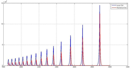
Figure 1. The graphical presentation of the approximate solution x of (9) and the exact solution.

5. Discussion

In this work, we proposed to study a non-linear sequential fractional problem associated with the (VdPL)-jerk equation. This problem is inspired by physics when we fall into the classical case. Then, we practically touched the analytical side, i.e., the analytical solvency (existence, uniqueness and stability of the solutions) for our problem according to the Caputo–Hadamard approach, using the Banach contraction principle, Krasnoselskii fixed-point theorem and Ulam–Hyers stabilities. An example was presented to illustrate the effectiveness of the results.

An interesting direction for future research of course would be to consider the numerical side and applications and try to use the theory of approximations to validate the results, which have already been treated analytically in this work as well as others.

References

- Abolfazl, J.; Hadi, F. The application of Duffing oscillator in weak signal detection. ECTI Trans. Electr. Eng. Electron. Commun. 2011, 9, 1–6. [Google Scholar]
- Alvarez-Ramirez, J.; Espinosa-Paredes, G.; Puebla, H. Chaos control using small-amplitude damping signals. Phys. Lett. 2003, 316, 196–205. [Google Scholar] [CrossRef]
- Ejikeme, C.L.; Oyesanya, M.O.; Agbebaku, D.F.; Okofu, M.B. Solution to nonlinear Duffing Oscillator with fractional derivatives using Homotopy Analysis Method (HAM). Glob. J. Pure Appl. Math. 2018, 14, 1363–1388. [Google Scholar]
- Dib, Y.O.E. Stability analysis of a strongly displacement time delayed Duffing oscillator using multiple scales homotopy perturbation method. J. Appl. Comput. Mech. 2018, 4, 260–274. [Google Scholar]
- Guitian, H.; Mao-kang, L. Dynamic behavior of fractional order Duffing chaotic system and its synchronization via singly active control. Appl. Math. Mech. Engl. Ed. 2012, 33, 567–582. [Google Scholar] [CrossRef]
- Ibrahim, R.W. Stability of A Fractional Differential Equation. Int. J. Math. Phys. Quantum Eng. 2013, 7, 300–305. [Google Scholar]
- Junyi, C.; Chengbin, M.; Xie, Z.J.H. Nonlinear Dynamics of Duffing System With Fractional Order Damping. J. Comput. Nonlinear Dyn. 2010, 5, 041012. [Google Scholar]
- Nikana, O.; Avazzadeh, Z. Numerical simulation of fractional evolution model arising in viscoelastic mechanics. Appl. Numer. Math. 2021, 169, 303–320. [Google Scholar] [CrossRef]
- Nikana, O.; Avazzadeh, Z.; Machado, J.A.T. Numerical approach for modeling fractional heat conduction in porous medium with the generalized Cattaneo model. Appl. Math. Model. 2021, 100, 107–124. [Google Scholar] [CrossRef]
- El-hady, E.; Ögrekçi, S. On Hyers-Ulam-Rassias stability of fractional differential equations with Caputo derivative. J. Math. Comput. Sci. 2021, 22, 325–332. [Google Scholar] [CrossRef]
- Kovacic, I.; Brennan, M.J. Nonlinear Oscillators and Their Behavior, 1st ed.; John Wiley and Sons: Hoboken, NJ, USA, 2011; ISBN 978-0-470-71549-9. [Google Scholar]
- Latif, M.A.; Chedjou, J.C.; Kyamakya, K. The paradigm of non-linear oscillators in image processing. In Proceedings of the In VXV International Symposium on Theoretical Engineering, Lübeck, Germany, 22–24 June 2009; pp. 1–5. [Google Scholar]
- Maimistov, A.I. Propagation of an ultimately short electromagnetic pulsein a nonlinear medium described by the fifth-Order Duffing model. Opt. Spectrosc. 2003, 94, 251–257. [Google Scholar] [CrossRef]
- Niu, J.; Liu, R.; Shen, Y.; Yang, S. Chaos detection of Duffing system with fractional-order derivative by Melnikov method. Chaos 2019, 29, 123106. [Google Scholar] [CrossRef] [PubMed]
- Pirmohabbati, P.; Sheikhani, A.H.R.; Najafi, H.S.; Ziabari, A.A. Numerical solution of full fractional Duffing equations with Cubic-Quintic-Heptic nonlinearities. J. AIMS Math. 2020, 5, 1621–1641. [Google Scholar] [CrossRef]
- Rhoads, J.F.; Shaw, S.W.; Turner, K.L. Nonlinear dynamics and its applications in Micro and Nano resonators. J. Dyn. Syst. Meas. Control. 2010, 132, 034001. [Google Scholar] [CrossRef]
- Sunday, J. The Duffing oscillator: Applications and computational simulations. Asian Res. J. Math. 2017, 2, 1–13. [Google Scholar] [CrossRef]
- Wagner, H. Large-Amplitude free vibrations of a beam. J. Appl. Mech. 1965, 32, 887–892. [Google Scholar] [CrossRef]
- Tamba, V.K.; Kingni, S.T.; Kuiate, G.F.; Fostsin, H.B.; Tallas, P.K. Coexistence of attractors in autonomous Van der Pol-Duffing jerk oscillator: Analysis, chaos control and synchronisation in its fractional-order form. Pramana—J. Phys. 2018, 91, 1–11. [Google Scholar] [CrossRef]
- Bezziou, M.; Jebril, I.H.; Dahmani, Z. A new nonlinear duffing system with sequential fractional derivatives. In Chaos, Solitons and Fractals; Elsevier: Amsterdam, The Netherlands, 2021. [Google Scholar]
- Dahmani, Z.; Belhamiti, M.M.; Sarikaya, M.Z. A Three Fractional Order Jerk Equation With Anti Periodic Conditions. submitted paper.
- Shammakh, W. A study of Caputo-Hadamard-Type fractional differential equations with nonlocal boundary conditions. J. Funct. Spaces 2016, 2016, 7057910. [Google Scholar] [CrossRef]
- Senouci, A.; Menacer, T. Control, Stabilization and Synchronization of Fractional-Order Jerk System. Nonlinear Dyn. Syst. Theory 2019, 19, 523–536. [Google Scholar]
- Jarad, F.; Abdeljawad, T.; Beleanu, D. Caputo-type modification of the Hadamard fractional derivative. Adv. Differ. Equ. 2012, 2012, 142. [Google Scholar] [CrossRef]
- Kilbas, A.A.; Srivastava, H.M.; Trujillo, J. Theory and Applications of Fractional Differential Equations; Elsevier: Amsterdam, The Netherlands, 2006. [Google Scholar]
- Miller, K.S.; Ross, B. An Introduction to the Fractional Calculus and Fractional Differential Equations; Wiley: New York, NY, USA, 1993. [Google Scholar]
- Brzdek, J.; Popa, D.; Rasa, I.; Xu, B. Ulam Stability of Operators; Academic Press: Cambridge, MA, USA; Elsevier: Oxford, UK, 2018. [Google Scholar]
- Shao, J.; Guo, B. Existence of Solutions and Hyers-Ulam Stability for a Coupled System of Nonlinear Fractional Differential Equations with p-Laplacian Operator. Symmetry 2021, 13, 1160. [Google Scholar] [CrossRef]
- Khan, H.; Li, Y.; Chen, W.; Baleanu, D.; Khan, A. Existence theorems and Hyers-Ulam stability for a coupled system of fractional differential equations with p-Laplacian operator. Bound Value Probl. 2017, 2017, 1–16. [Google Scholar] [CrossRef]
- El-Sayed, A.; El-Raheem, Z.; Salman, S. Discretization of forced Duffing system with fractional-order damping. Adv. Differ. Equ. 2014, 2014, 66. [Google Scholar] [CrossRef]
- Bezziou, M.; Dahmani, Z.; Jebril, I.; Belhamiti, M.M. Solvability for a Differential System of Duffing Type Via Caputo-Hadamard Approach. Appl. Math. Inf. Sci. 2022, 16, 341–352. [Google Scholar]
Publisher’s Note: MDPI stays neutral with regard to jurisdictional claims in published maps and institutional affiliations. |
© 2022 by the authors. Licensee MDPI, Basel, Switzerland. This article is an open access article distributed under the terms and conditions of the Creative Commons Attribution (CC BY) license (https://creativecommons.org/licenses/by/4.0/).