Abstract
The assembly quality of a complex product is the result of the combined effects of multiple manufacturing stages, including design, machining and assembly, and it is influenced by associated elements with complex coupling mechanisms. These elements generate and transmit assembly quality deviations during the assembly process which are difficult to analyze and express effectively. Current studies have focused on the analysis and optimization of the assembly surface errors of single or few components, while lacking attention to the impact of errors on the whole product. Therefore, in order to solve the above problem, an assembly quality deviation analysis (AQDA) model is constructed in this paper to analyze the deviation transfer process in the assembly process of complex products and to obtain the key features to optimize. Firstly, the assembly process information is extracted and the assembly quality network model is established on the basis of complex networks. Second, the Jacobian-Torsor (J-T) model is introduced to form a network edge weighting method suitable for the assembly process to objectively express the error propagation among product part features. Third, an error propagation model (EPM) is designed to simulate the error propagation and diffusion processes in the assembly network. Finally, the assembly process of an aero-engine fan rotor is used as an example for modeling and analysis. The results show that the proposed method can effectively identify the key assembly features in the assembly process of complex products and determine the key quality optimization points and monitoring points of the products, which can provide a decision basis for product quality optimization and control.
MSC:
05C82
1. Introduction
As the final link in the product manufacturing process, the assembly has a significant impact on the final quality of the product [1], and it is also one of the most costly links in the entire manufacturing process. Complex products are products with many parts, complex manufacturing processes, rich hierarchies and various changes between the parts and the whole. Products such as engines and turbines have the characteristics of high assembly difficulty and long assembly chains [2], and their assembly quality is affected by multiple factors such as design, processing, assembly, and testing [3], which makes assembly quality data have the characteristics of multiple sources, heterogeneity, and fragmentation [4]. Due to the numerous factors related to the assembly quality and the complex coupling mechanism between them, it is very difficult to analyze, monitor, and predict the assembly quality, which is manifested by unstable assembly quality, low one-time success rate, and reliance on workers’ experience for quality control.
Assembly quality deviations are not only caused by geometrical deviations of components [5], but also by deformations caused by positioning fixtures [6], assembly stress [7], and temperature [8]. The current research on the propagation and diffusion of assembly quality deviations still lacks a clear mechanism and an accurate model [9], resulting in a lack of theoretical guidance for the precision design and quality optimization of product parts. Even if the quality of each part meets the design requirements, errors will still gradually accumulate and spread during the assembly process, which ultimately make it difficult to guarantee the quality of the product. To ensure the stable performance of the assembled product, it is necessary to study the propagation and diffusion mechanism of errors during the assembly process, identify the key component features that affect the assembly quality, and trace the error source of the key features to effectively control the assembly quality. The quality of key assembly features and error sources is controlled to improve assembly efficiency and the one-time assembly success rate, which can save assembly costs. To ensure the quality of the final product, many scholars have conducted significant research on how to analyze and control the assembly quality of complex products.
In terms of assembly accuracy analysis methods, some scholars primarily study how to express the propagation process of deviations between parts by introducing the state-space equation in modern control theory for modeling to express the relationship between the features, forming an error flow model in the assembly process [10,11]. Other scholars use state-space equation modeling for the assembly process of precision machine tools to analyze the influence of deviation on the accuracy of the whole machine, and obtain the decision-making plan for assembly adjustment through optimal state estimation and optimal control methods [12,13]. Beruvides et al. [14] modeled the surface roughness using an adaptive neuro-fuzzy inference system and optimized it using a multi-objective genetic algorithm to form a system for monitoring and optimizing the surface roughness of the part. Shahi et al. [15] constructed the error propagation model in the multi-station linear assembly process, considering the spring-back phenomenon and the relocation error between the stations. The results showed that the stiffness and error of the parts have a significant impact on the assembly success rate. Liu et al. [16] analyzed the propagation process of mass eccentricity deviation in assembly and optimized the initial imbalance of the assembled rotor by appropriately selecting the assembly phase of the multi-stage rotor, which improved the assembly quality of the multi-stage rotor in the aero-engine assembly and can be used for assembly guidance, tolerance distribution, etc. Zhou et al. [17] analyzed the error modeling of the special equipment for the aero-engine rotor docking assembly process and proposed an error compensation method to improve the docking accuracy and success rate. Cai et al. [18] used an improved principal component analysis method to assess the deflection quality of the assembly car body, providing a basis for using specific data to assess properties of a particular product. Other scholars have applied the small displacement torsor model from robotics to tolerance modeling to express the variation of geometric features in the tolerance domain range [19,20,21]. Ding et al. [22] modeled the deviation of the aero-engine multi-stage rotor based on the J-T model, constructed the deviation transfer function and proposed a method for optimizing the assembly phase. Such methods can consider the influence of geometric deviations in the propagation of assembly quality deviations, but they are mostly based on rigid-body assumptions, and the influence of non-geometric factors such as stress and deformation cannot be fully considered. At the same time, the modeling principle is complicated, and it is difficult to fully consider complex products which cannot effectively express the coupling influence relationship among errors.
The assembly accuracy optimization method requires a lot of analysis and calculations. When the object is a complex product with many parts, the calculation for the whole product is large and difficult. To analyze and control the assembly quality in a faster and less costly way, it is necessary to find the features of the parts that have a greater impact on the whole assembly. In this case, this includes the geometric features of the parts that are involved in the assembly process and are related to the deviation. Finding the most influential assembly features and specifically controlling the quality of these features can optimize the resource allocation while improving the assembly quality. Such features are key assembly features. Thornton [23] proposed a mathematical definition of key features and a method to quantitatively identify key features to determine the objects that should be prioritized for quality control in assembly quality optimization. Whitney et al. [24] pointed out the importance of key features in the field of mechanical assembly, where improving product quality depends on finding critical dimensional, tolerance, and functional characteristics in the assembly. Han et al. [25] proposed a method to identify key assembly features in the assembly model from the perspective of assembly topology and multi-source attributes, and then proposed a two-level evaluation model to evaluate the importance of assembly parts and thus obtain the critical functional parts in the assembly. Li et al. [26] used the weighted LeaderRank algorithm and the susceptibility-infection-recovery (SIR) model of weighted directed complex networks to determine the influential (i.e., critical) functional modules of complex products and systems during the conceptual design phase. It can be seen that finding the key assembly features in the assembly quality analysis, and then performing an accuracy analysis and quality control on the associated assembly process can more efficiently improve the assembly quality and assembly efficiency, which can reduce assembly costs.
The nodes and edges in the complex network can visually express the correlation between many assembly features of complex products. The strength and path of error transmission can be reflected by the weight of edges in the network. The propagation of the error in assembly is analogous to the propagation of viruses in the human population. The propagation of assembly errors in the network is analyzed to find the error source nodes that are easier to propagate the error for focused monitoring. Previously, most studies have applied complex network methods to the machining and manufacturing processes. Daoyu et al. [27] established a machining error transfer network to identify weak nodes in the process flow as a basis for process improvement. They then introduced quality features into the machining error network to describe the influence relationships between nodes and combined this with the support vector regression machine algorithm to construct a multi-process processing quality prediction model [28]. The above methods are mainly used to model and analyze the machining process of complex products in combination with complex networks, while the assembly process, which is also a manufacturing stage, presents unclear mechanisms for the evolution of assembly quality deviations compared with the machining process. The low level of automation and digitization in the assembly process has resulted in the lack of specific and measurable indicators for individual parts and the whole, so it is difficult to apply the above methods directly to the assembly process [29]. Peng et al. [30] combined the assembly process, assembly features, and their actual measurement data together to establish an assembly deviation transfer network which could identify the KF nodes, and proposed a reverse backtracking algorithm to identify the error sources. Hong et al. [31] deeply analyzed the principle of fluctuating transmission of machining errors and constructed a weighted network model which realized the identification of network key nodes and applied the breadth-first search strategy to identify the fluctuation source. Verna et al. [32] designed an assembly quality inspection strategy framework for low-volume production and proposed an inspection strategy map to evaluate and predict quality defects to help designers make decisions. Jiakun et al. [33] established a hierarchical weighted network including a part layer and a feature layer based on the assembly relationship and indirect relationship, and proposed an improved association detection algorithm to classify the assembled part units. Although the above methods applied complex network methods to the assembly process, they have not been able to express the propagation of errors reasonably and objectively. An accurate study of the propagation of quality deviations in the assembly process is particularly important to help researchers to identify critical assembly parts.
This paper proposes an EPM-based AQDA method that makes it more efficient to utilize complex networks to analyze assembly error propagation in the assembly process. We extend the idea of [33] which constructed complex networks based on parts and features to determine network nodes, and define the direction of edges according to the assembly process. For the influence of errors between nodes, most of the existing methods use subjective methods such as expert scoring or AHP to give weights, which leads to the analysis results relying on human experience. We introduce the J-T model from the precision analysis method as an objective expression of the influence relationship between nodes. Then, referring to the SIR model, the error propagation process between parts is represented by probability. After analyzing the network characteristics of the obtained results, we define new node properties for identifying key nodes which is more suitable for assembly error propagation analysis.
The main work of this paper is summarized as follows: firstly, the information of the assembly process is mapped into a complex network to form an AQDA network; secondly, the error propagation magnitude among the feature nodes is calculated by the J-T model, and the edge weights are assigned accordingly; finally, an EPM is constructed to analyze the key feature nodes in the network, and the effectiveness of the proposed method is verified on an aero-engine multi-stage rotor. The rest of the paper is organized as follows. The section “Preliminaries” describes the definitions and principles related to complex networks, J-T model, and so on. Section “Methodology” explains the process and specific details of the proposed method. Section “Case Study” validates the proposed method by applying the EPM in an example, and the last section concludes this article.
2. Preliminaries
2.1. Complex Network
Complex network is a network graph that reflects the intricate topology and association relationships in a complex system, and consists of nodes and edges connecting these nodes, defined as the graph , where is the nodes in the graph, and refers to the existence of an edge between nodes and (if is a directed graph, then is the existence of an edge between nodes and that points from to ). The association can also be expressed by an adjacency matrix, i.e., a matrix with elements, where the elements are defined as follows:
where is the weight of the edge between node and node , if is an unweighted graph takes the value of 1.
2.2. Jacobian-Torsor Model
The torsor model was first used to describe the positional transformations of an object. The motion of an object in a positional transformation can be decomposed into a rotation around a line and a horizontal movement along that line, and this compound motion becomes a spiral motion. In an advanced study of the spiral motion, ref. [34] applied the torsor model to the tolerance model for expressing the tolerance by defining the geometric center of a geometric feature as the origin of the coordinate system, and for the ideal position of the geometric feature, the deviation of its changed position with respect to can be decomposed into a translation vector along the coordinate axis and a rotation vector around the coordinate axis , the schematic diagram of which is shown in Figure 1, and the expression form of the torsor model is as follows:
where , , are the amount of translational movement of the geometric feature along the axes , , and , , are the amount of rotation of the geometric feature along the axes , , .
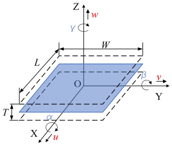
Figure 1.
Schematic diagram of the torsor model.
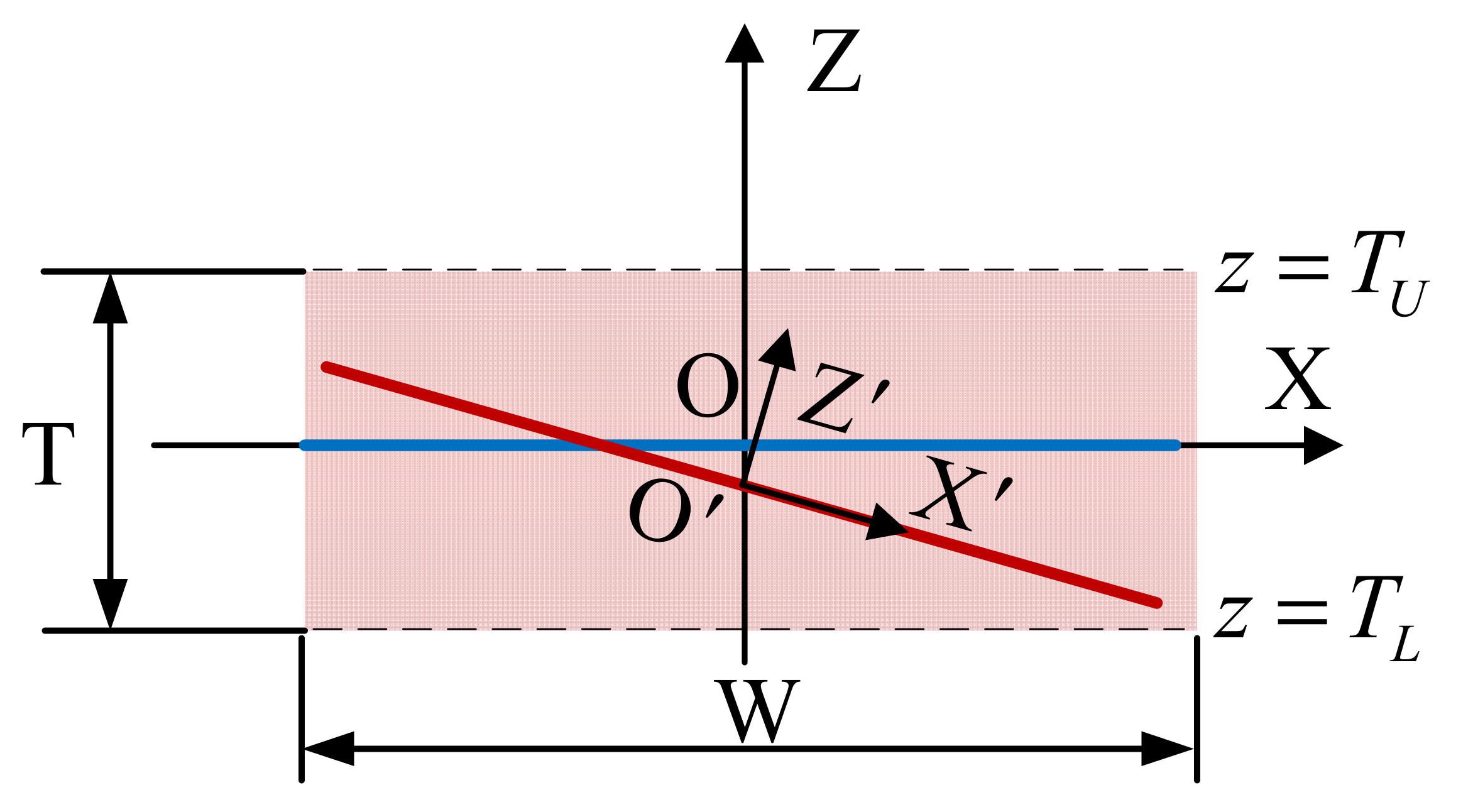
The tolerance zone is the region where the actual geometric features are allowed to vary and is a closed spatial region enclosed by boundary surfaces or boundary lines. Chen et al. [35] summarized the tolerance zones of various geometric features. Only the common planar features and cylindrical features are described here. The planar feature has three degrees of freedom (DOF), namely, translation along the axis , rotation along the axis , and rotation along the axis , and the remaining three vectors are 0. The planar feature is bounded by the position tolerance, and lets the variation range of the translation along the axis be the position tolerance T. The upper and lower bound of the planar feature along the axis is set to and , and it is known that , and the tolerance zone of the planar feature is the space region between two parallel planes at a distance T. For the rotation along the axis and the rotation along the axis , the range of variation is and , and L and W are the lengths of the plane features along the axis and the axis respectively, as can be seen from Figure 2.
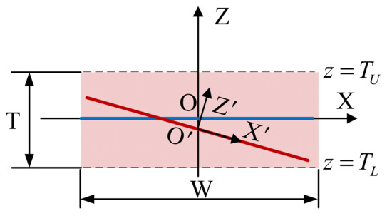
Figure 2.
Range of variation of plane features in the x-z plane.
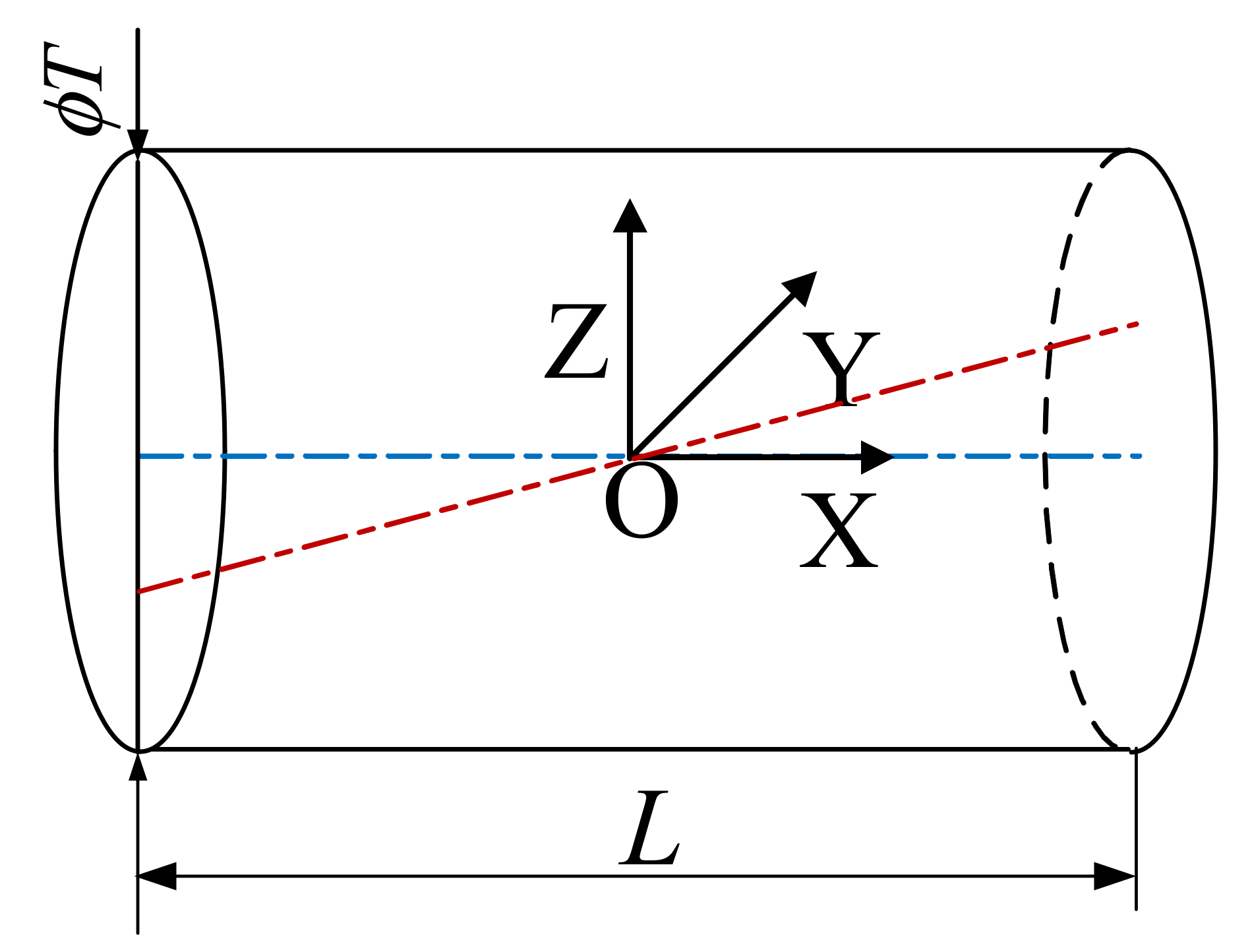
The cylindrical axis feature has 4 DOF, namely, translation along the axis , translation along the axis , rotation along the axis , rotation along the axis , and the remaining two vectors are 0. The cylindrical axis feature is constrained by the coaxiality and other positional tolerances, let the tolerance range of the coaxiality that limits the cylindrical axis feature be , and the length of its axis is . Its tolerance zone is the cylindrical region as shown in Figure 3, and the range of variation of its torsors can be seen from Figure 3 as , , , .
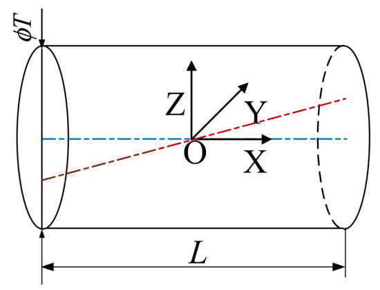
Figure 3.
Variation of the spin volume of the cylindrical axis feature.
The Jacobian matrix originated from robotics for transferring the poses and velocities of each joint. Laperrière and Lafond [36] introduced it into the tolerance model for transferring the rotations and translations of the geometric features in the tolerance domain. The amount of movement and rotation of the feature in the global coordinate system can be transferred by the Jacobian matrix. The amount of movement of the local coordinate system with respect to the origin of the global coordinate system can be directly accumulated along the three coordinate axis directions, with no effect on the amount of rotation, and the conversion matrix for the conversion of the feature from the local to the global coordinate system is:
where , , are the unit direction vector of the local coordinate system with respect to each of the three axes of the global coordinate system .
For the rotation of the local coordinate system with respect to the target coordinate system , it is obtained from the vector product of and the distance between the origin of the local coordinate system and the rotating target point , and is calculated as:
where is calculated from , and .
The complete Jacobian matrix of the local coordinate system with respect to the global coordinate system is the combination of the two as follows:
The J-T model combines the characteristics of the above two models, expresses the tolerance using the torsor model, and transfers the tolerance using the Jacobian matrix. The product of the Jacobian matrix and the corresponding change torsor is the effect of the change of a feature relative to the origin of the global coordinate system [37]. For a target feature (called functional requirement (FR) in the J-T model), its change with respect to the origin of the global coordinate system should be the result of the superposition of the changes of its related features (called functional elements (FE) in the J-T model), i.e., the J-T model of the FR is expressed as follows:
3. Methodology
To address the problem of lack of effective and objective analysis methods for complex product assembly quality, this paper uses complex networks for the construction of the AQDA model combined with the J-T model to assign weights to the edges of the network, based on which an EPM is constructed for AQDA in order to provide key optimization and monitoring objects for enhancing and improving product assembly quality. Firstly, the assembly process information is extracted and the assembly process is mapped into a complex network. Secondly, the J-T model is calculated between the feature nodes with edges, and the results of the J-T model are transformed into edge weights. Finally, the EPM is used to show the deviation propagation diffusion process and identify the KAF nodes.
3.1. Complex Network Module for Assembly Quality Analysis
According to the assembly process specification and other technical documents to extract parts information and feature information, according to the correlation between the information to build a complex network model: for a part with multiple feature surfaces involved in the assembly, each of these feature surfaces is treated as a node because the work steps they are involved in and the parts they are associated with may be different. For a part with only one feature surface involved in the assembly, the part is directly used as a node. For identical parts with a quantity greater than one, the same function and in the same work step in the assembly, such as multiple blades installed in the same position along the radial direction in rotary machinery, they are identified as the same node to avoid the degree of their associated nodes being too large, which affects the results of network characteristic analysis.
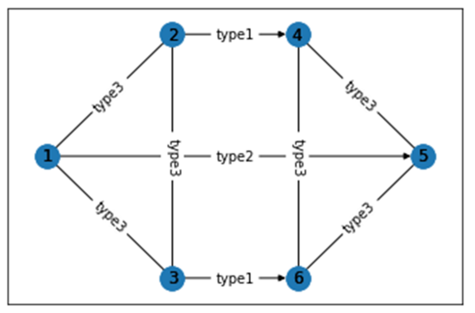
The connection relationship between the nodes is determined based on the relationship between the parts in the assembly. The relationship between features mainly includes three relationships, as shown in Figure 4. Type 1 indicates the mating relationship between parts, using a directed edge from the first assembly features to the later assembly features. Type 2 indicates a benchmark relationship, such as a feature for another feature assembly benchmark, or the existence of form tolerance requirements between features, etc., using a directed edge from the benchmark features to the features with form requirements. Type 3 indicates that when different features on the same part are each involved in the assembly, they are connected by an undirected edge. The specific relationship can be added or deleted according to the actual assembly process of the product.
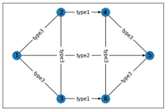
Figure 4.
Assembly quality analysis network model. Type1.
According to the above principles, we can establish a complex network graph corresponding to the actual assembly process, where is all the part nodes or feature nodes involved in the assembly, and according to the relationship between the parts to form an edge, refers to the existence of an edge between nodes and (if is a directed edge refers to the existence of an edge between nodes and that points from to ).
3.2. Assigning Weights to Edges Based on the J-T Model
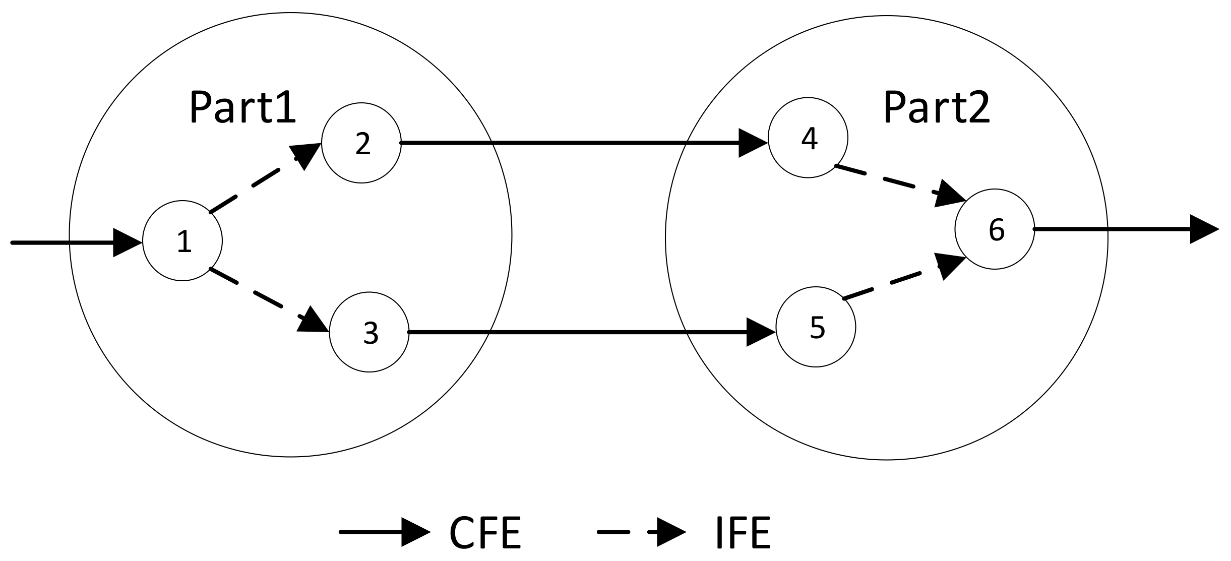
In the J-T model, the two features on the same part that have a mutually constraining relationship are called the internal functional element (IFE), and the two features on different parts that have a direct or indirect contact relationship are called the contact functional element (CFE), according to which the assembly connection diagram is formed, as shown in Figure 5. The edges of the nodes in the network model can be expressed by the combination of IFE or CFE in their paths. Therefore, using the J-T model to express the exact tolerance and error transfer of the features, we can calculate the magnitude of error transfer between the associated features in the network model by the Jacobian matrix and torsors. Assuming that the edges between the two associated features are directed edges , the center of the starting feature is used as the origin of the coordinate system, and the ending feature is used as the FR, the J-T model of the FR is calculated as follows:
where is the Jacobian matrix of the errors transmitted by the related features associated in the path from feature to feature , and the matrix on the right-hand side is the variation torsors of the related features. In the th column vector , the , , and are the translations of the th FE along the coordinate axis with respect to the th FE as the origin of the coordinate axis, and , and are the rotations of the (k + 1)st FE along the coordinate axis with respect to the center of th FE as the origin of the coordinate axis.
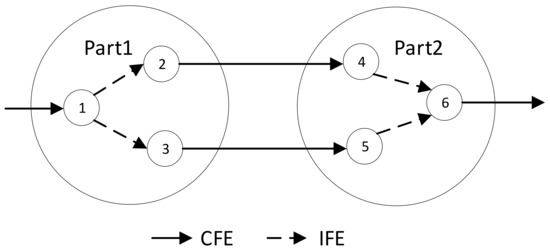
Figure 5.
Assembly connection relationship diagram.
The , and of the final derived FR are the translational motions of feature along coordinate axes , , with respect to global coordinate system origin (the center of feature ), and , and are the rotations of feature along coordinate axes , , with respect to global coordinate system origin. Their magnitudes are and respectively, and the magnitude of their absolute values represents the deviations they contain in their respective dimensions. Considering that the six-dimensional data are three rotational degrees of freedom and translational degrees of freedom, which are mutually perpendicular and independent in Euclidean space, the correlation between them can be neglected. To express the magnitude of the transmitted errors in a comprehensive way, we normalize the six-dimensional data by min-max methods to fall within the interval respectively, which is calculated as:
where , are the upper and lower limits of the independent variation range of each vector. The purpose of min-max normalization is to remove the unit constraints of the data and transform them into pure values of magnitude, so that metrics of different units of magnitude can be easily compared.
The normalized data can be summed up to obtain one-dimensional data, which is used as the error magnitude transmitted by the feature to the feature , is a value between , which can be directly used as the weight of the edge.
When the relationship between features is a benchmark relationship or belongs to the same part, it is easy to get the weight of the edge between two features by the above method. For the mating relationship between parts, such as the interference fit relationship between shaft and hole, which is a fixed contact pair and no variation is introduced, we set its weight as 1 and consider its edge as the connecting effect, which does not have a reducing or amplifying effect on the error.
3.3. Key Node Identification Based on Probability Propagation Model
In order to study the influence of assembly quality deviation propagation diffusion behavior in network models, an EPM of assembly errors is constructed by combining the actual process of complex product assembly. In reality, the propagation behavior exists on network models in many fields, such as disease propagation in social networks, virus propagation in communication networks, and successive failures in power networks, etc. The EPM constructed in this paper is inspired by, but not identical to, the above models. The assembly process of complex mechanical products is a discrete process containing a finite number of work steps, and only some parts in each work step are involved in the assembly. According to the characteristics of the assembly, the model is constructed according to the following conditions. The schematic diagram of the error propagation process of the th step is shown in Figure 6.
- (1)
- All feature nodes in the network model are initially in the normal state, represented by N, and initially carry an error of 0. Feature nodes affected by the propagation of the assembly error are transformed into the infected state, represented by .
- (2)
- The model runs in unit time as work steps, and in each work step, only the assembly feature nodes involved in that work step are capable of propagating the error.
- (3)
- The probability of propagation of the error from the infected node to the associated node is the variance of the weights of the edges between the two nodes.
- (4)
- In propagating the error, the error of the infected node is the sum of the error of the infected node and the weights of the connected edges.
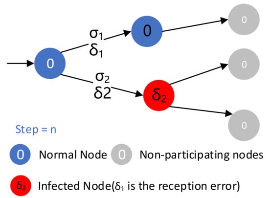
Figure 6.
Probabilistic propagation model propagation process for the nth work step.

In the actual assembly, this EPM is run after assigning weights to the edges of the network model based on the dimensional and form tolerance data of the product part features, and it can observe the propagation and spread of quality errors during the assembly process. Since the error propagation is probability propagation, the results of each run may vary to a certain extent, and statistical analysis of the EPM after several runs can obtain a more stable and reliable result. In the process of error propagation and diffusion, the nodes that should be focused on can be divided into two categories. One is the nodes with more cumulative transmission errors (CTEs); such nodes are often error sources or important hub nodes. The quality optimization of the corresponding features of such nodes or improving their quality requirements can effectively reduce the generation of errors. The other is the nodes with more cumulative reception errors (CRE); such nodes are greatly affected by the errors and are more likely to exceed the quality requirements and fail. Monitoring the corresponding feature of such nodes can effectively determine the quality status of the entire product assembly process.
4. Case Study
As one of the core components of an aero-engine, the assembly quality of the fan rotor has an important impact on the service quality of the whole aero-engine after assembly; such as excessive imbalance of the fan rotor assembly will lead to the reduction of the reliability and remaining life of the whole aero-engine. And in serious cases, the rotor will produce severe vibration in operation, which may reduce efficiency and even cause accidents. In this paper, the fan rotor assembly of an aero-engine is selected as the research object for modeling and analysis.
4.1. Approaches Implementation
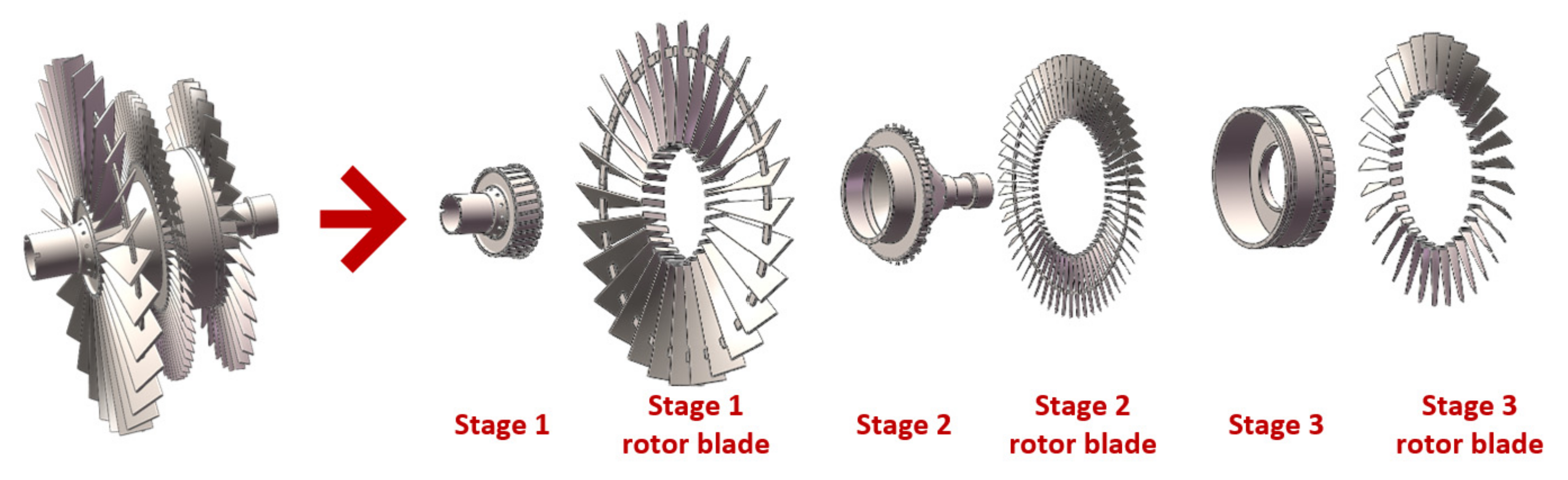
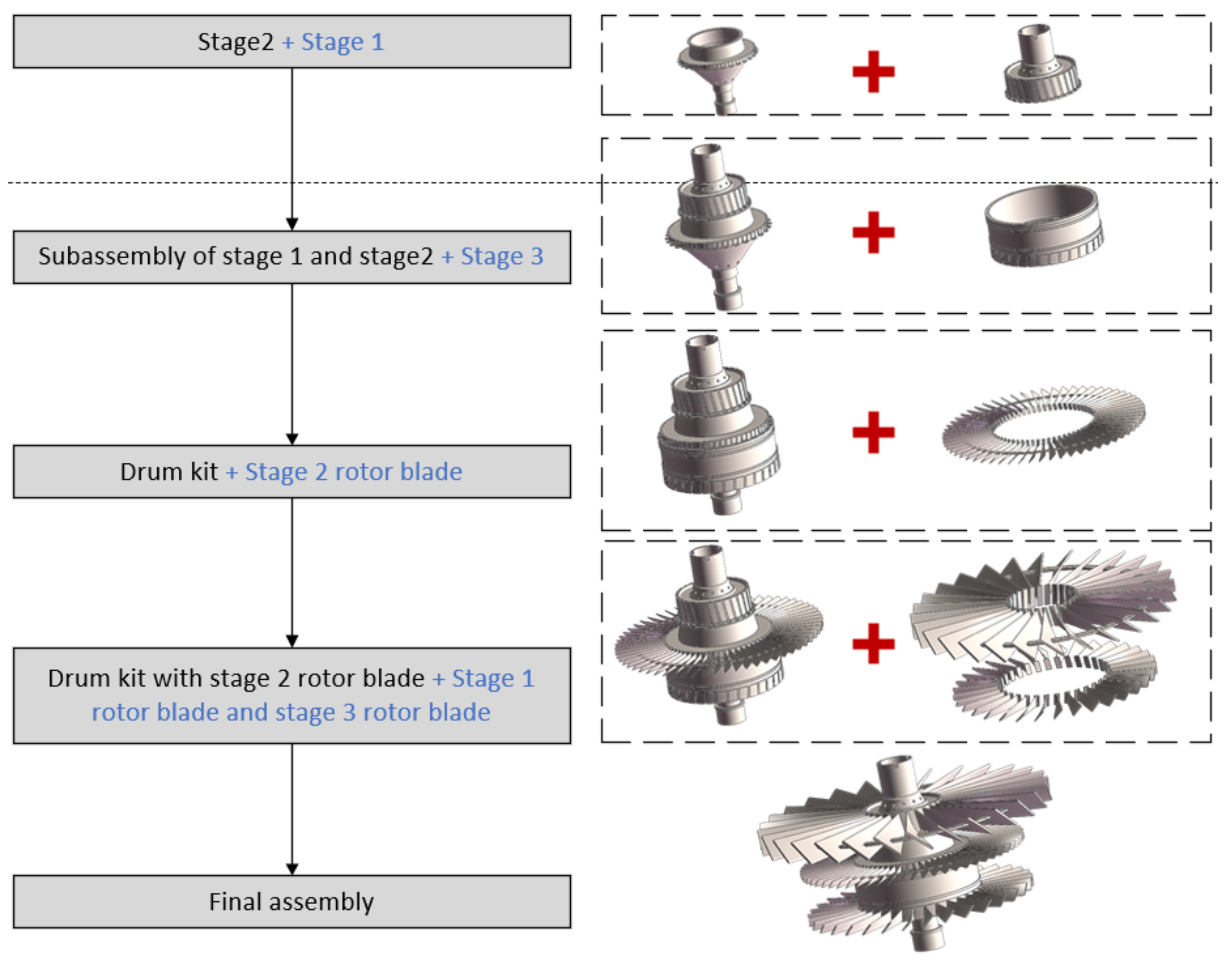
The rotor studied in this paper is a fan rotor with a three-stage disc drum which can be divided into three parts: stage 1 unit, stage 2 unit and stage 3 unit. Each unit consists of a drum and the vanes, bolts, etc. mounted on it. The connection between the different units is formed by multiple feature face contacts and bolted connections on the disc drum. Each feature surface on the drum that participates in the connection should be determined as a feature node. Figure 7 shows the main components of the research object. Connections such as bolts and supports such as bearings are omitted from the figure. Figure 8 shows the assembly process of the research object, in which each step is to install the right part (marked in blue) based on the left part (marked in black). Parts involved in the assembly process can be determined according to the bill of materials. The actual features of each part can be clarified according to technical documents such as assembly process specifications. So that the nodes of the AQDA network can be generated as mentioned in Section 3.1. The network model nodes and corresponding features are shown in Table 1, which shows the non-exact names of parts and part features.

Figure 7.
Main components of the fan rotor.
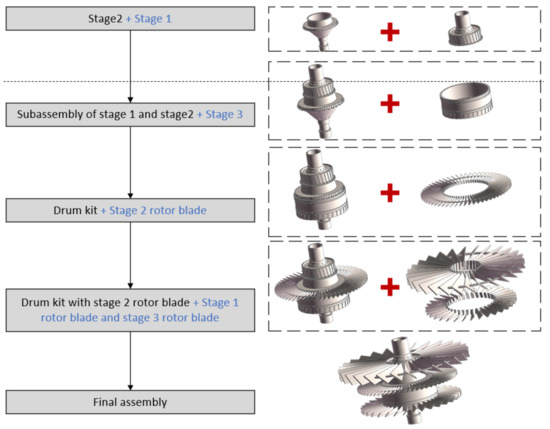
Figure 8.
The assembly process of the fan rotor.

Table 1.
Correspondence between node naming and representative part features.
Since the research object in this paper is the rotor part of an aero-engine which does not include the static sub-part such as the magazine, the main association relations of the edges in the network model are the mating relationship (type1), the benchmark relationship (type2) and on the same part (type3). When assigning weights to the network, if the geometric dimensions, dimensional tolerances, and form tolerance requirements in the design stage are used as inputs, the distribution of errors can be simulated by Monte Carlo simulation, the results of the J-T model can be used to assign weights to edges through multiple simulations, and the average statistical weights can be used to examine the average impact of errors generated by each component in the whole assembly process, which can point out the optimization focus for each feature in the design phase. If the actual data is measured in the assembly stage, the actual error can be directly inputted into the J-T model to calculate the size of error transmission, then the edge weight reflects the actual situation of error transmission between features in this assembly and is used to analyze the influence of the error generated by each feature in this assembly. In this paper, simulation data were generated according to the measured dimensional distribution according to the actual tolerance requirements. In actual production, for the same batch of parts machined by machine tools, their dimensional errors, the same accuracy under repeated measurements generated by the measurement error, are approximately obeyed by the normal distribution, so we assume that the variation in the amount of torsor and dimensional change parameters of each feature are subject to the normal distribution; the distribution of the mean and standard deviation is calculated as follows:
where and are the upper and lower bounds of each torsor component, Z is the standard normal number, and should be taken according to the three-sigma rule.
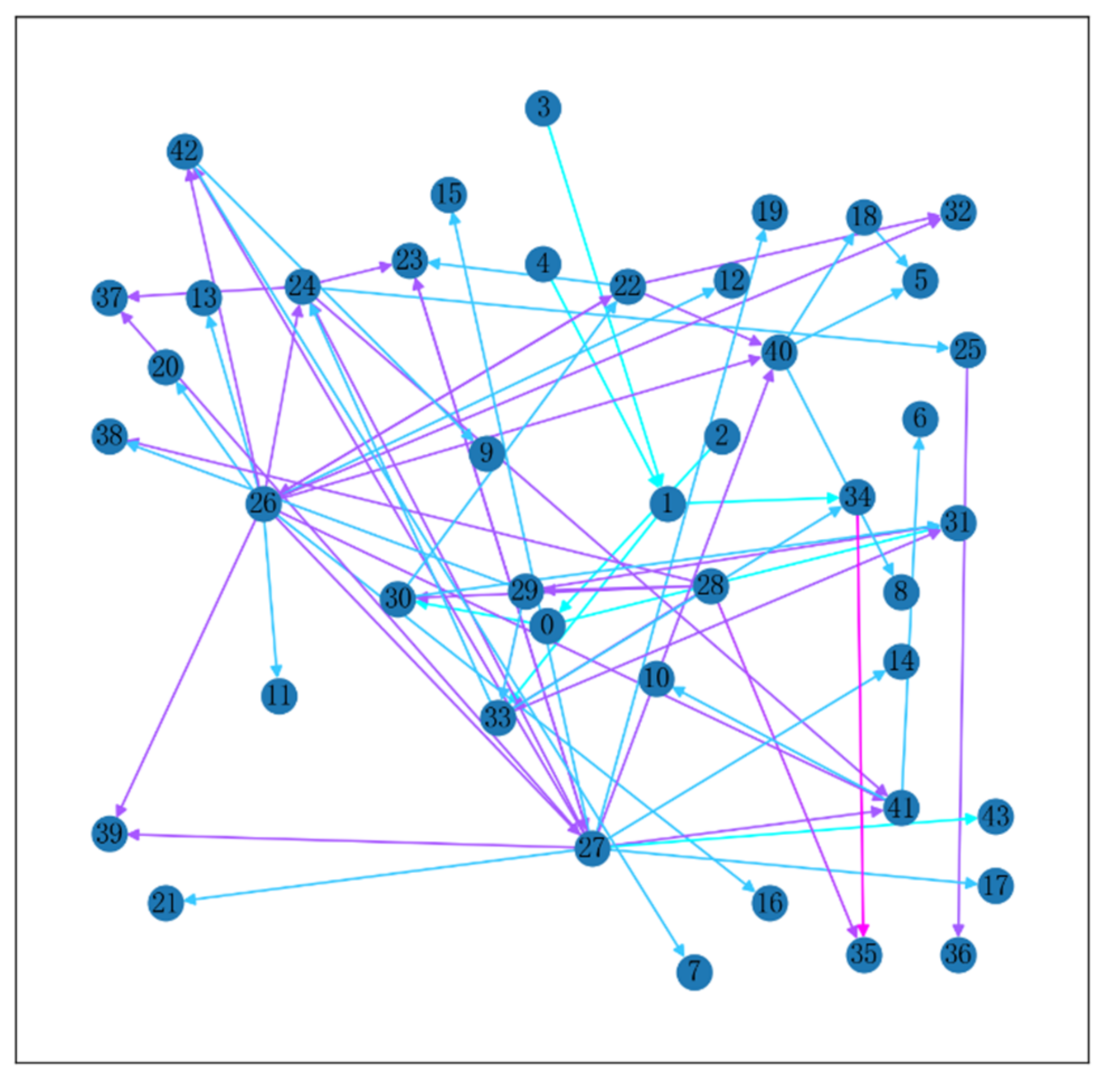
The network model is shown in Figure 9; the closer the edge color is to blue, the smaller the weight, and the closer the edge color is to purple, the larger the weight.

Figure 9.
Assembly error network simulated by the probability propagation model (the closer the edge color is to blue, the smaller the weight, and the closer the edge color is to purple, the larger the weight).
After building a directed weighted network, the statistical characteristics of the network can be analyzed first to understand the local nature of nodes. There are many algorithms for mining the importance of nodes, including node degree centrality (based on node nearest neighbors), betweenness centrality (based on paths), closeness centrality (based on paths), eigenvector centrality (considering the number and quality of node nearest neighbors), etc. The top 10 nodes and corresponding values of each metric in the network are shown in Table 2. These metrics can reflect the scope, speed, and degree of influence of nodes in the propagation of assembly quality deviations from their respective perspectives. The nodes with a high degree centrality will affect more nodes after the error is generated due to their many associated nodes. The nodes with high betweenness centrality are on multiple propagation paths, and when their errors increase, they will affect the errors of downstream nodes. Closeness centrality considers the distance of each node to reach other nodes, and the nodes that are closer to all other nodes will not weaken the quality relationship when the propagation of their errors is due to more transmission links on the path. Eigenvector centrality considers the quality of the nodes associated with each node, and the higher the quality of the associated nodes, the more important they are, and the impact of the nodes thus identified in generating errors has a more significant effect on assembly quality.
Table 2.
Node importance index values for assembly quality analysis model.
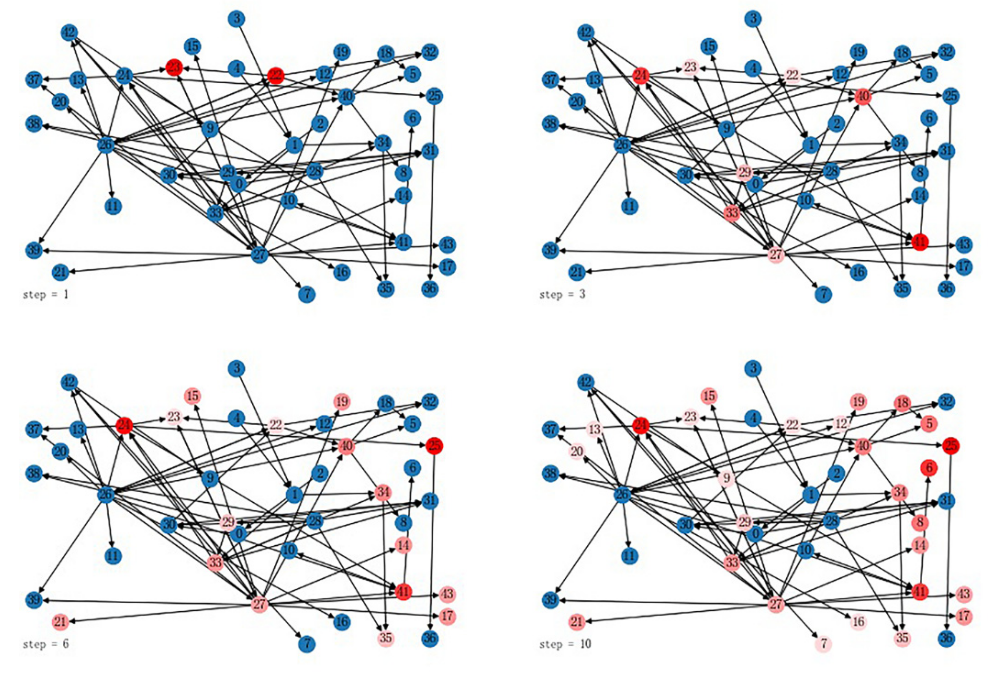
The assembly features involved in each work step are input into the EPM for simulation based on the assembly process information. The single assembly error propagation process of the fan rotor is shown in Figure 10. It contains 11 steps of the assembly process, only four of which are selected for demonstration. The results of the statistical analysis after 10,000 simulation runs are shown in Figure 11. The closer the node is to blue means its CRE is close to 0, and the closer it is to red means its CRE is larger. In order to determine nodes with high CTE or high CRE, it is necessary to set the threshold for division, which can be manually set or calculated by clustering algorithms. Considering the influence of subjective factors brought by artificially setting thresholds, the clustering method is selected to obtain the required thresholds and division results. K-means is a partition-based clustering method that is characterized by simplicity and efficiency. Its performance is sufficient to correctly handle 2D datasets of EPM results. By clustering the nodes in k-means, the nodes can be divided into three categories as shown in Figure 12. As mentioned before, the node corresponding to the feature with the largest average CTE should be used as a control point for quality optimization, and the resulting error should be reduced by improving its quality requirements and accuracy requirements. The node with the largest average CRE, by monitoring the changes in its quality characteristics during the assembly process, such as runout, coaxiality, and other form errors, can determine the quality status of the current assembly process, and when it is close to or exceeds the tolerance requirements, the assembly process should be stopped in time and adjusted to reduce errors and improve quality through repair and other methods.
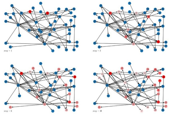
Figure 10.
Single assembly error probability propagation process.
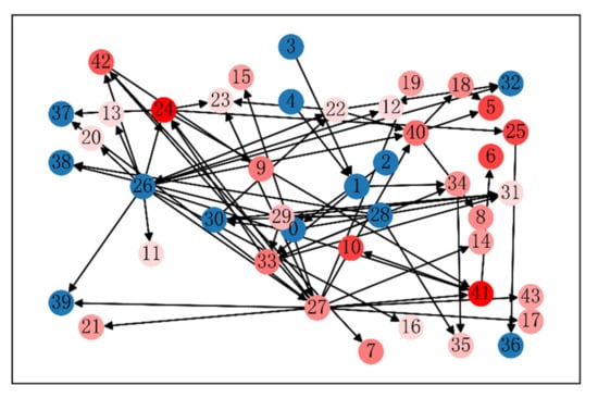
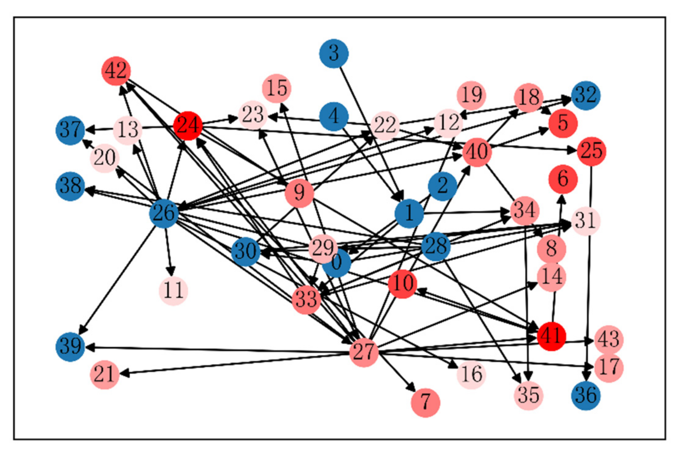
Figure 11.
CRE results of the probability propagation model (the closer the node is to blue means its CRE is close to 0, and the closer it is to red means its CRE is larger).

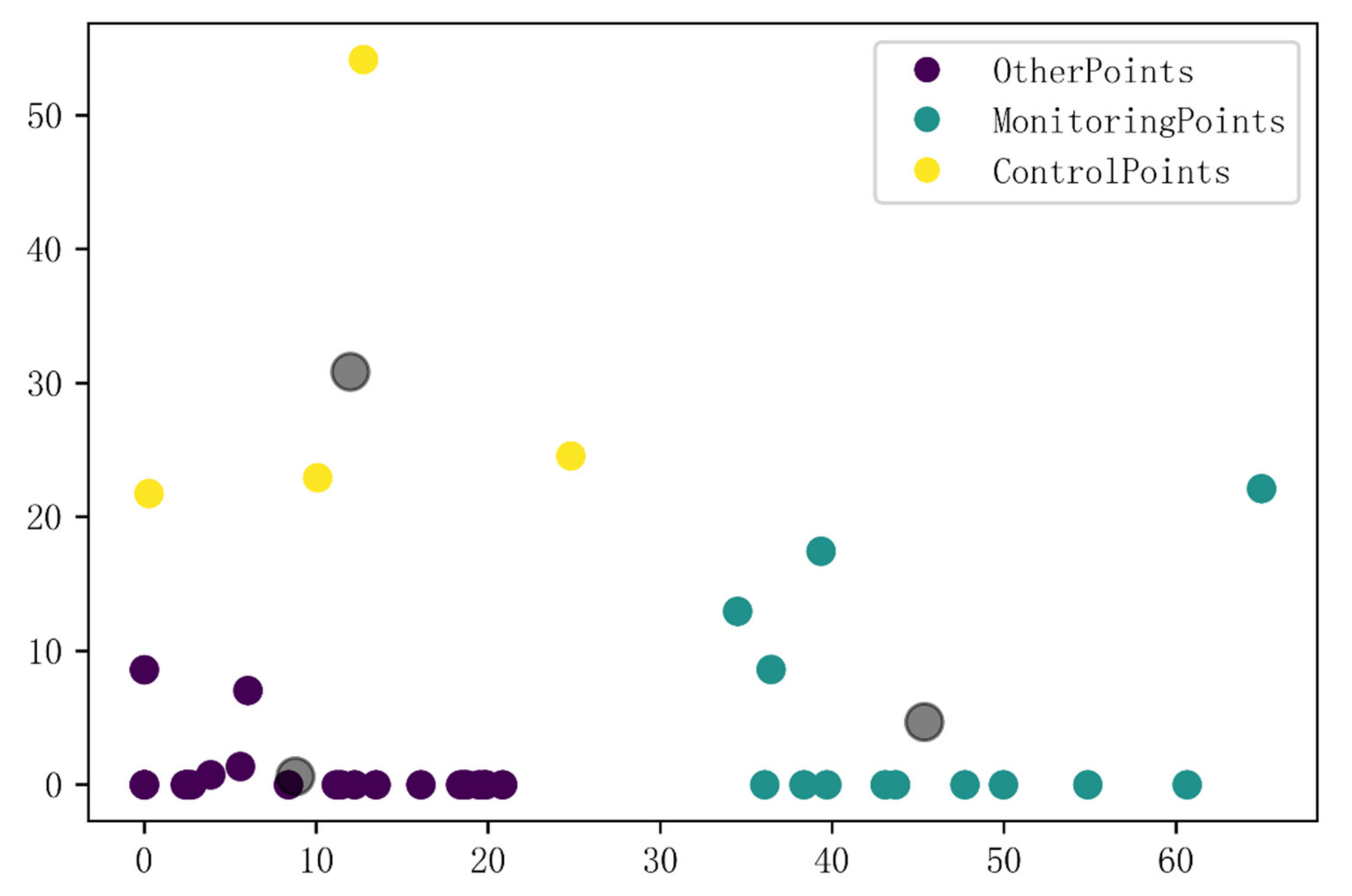
Figure 12.
k-means clustering results (the gray dots are the centroids of each category identified by the clustering algorithm).
4.2. Discussion
Nodes that get higher values in the EPM are often also located in the top positions in the results of the important node, as shown in Table 2. Comparing the top five nodes of CRE and CTE in the EPM results as shown in Table 3 (9 nodes in total, node 41 is in both rankings) with the top 10 nodes of different node importance metrics in Table 2, the number of nodes that agree are: degree centrality: six, betweenness centrality: five, closeness centrality: six, and eigenvector centrality: seven. However, the results of the traditional node importance ranking method can determine the importance of the nodes, but cannot discover further properties of feature nodes, and cannot distinguish whether the nodes should be classified as control points or monitoring points.
Table 3.
Top 5 nodes in CRE and CTE.
Combined with the actual analysis of the EPM results obtained in Table 3, the average CTE top5 nodes are the verified rotor’s stage 2 disc journal outer circle (node 27), stage 2 rear stop end face (node 33), stage 2 inner diameter of rear stop (node 24), stage 1 disk journal outer circle (node 26), and stage 2 disk rim (node 41). The stage 2 disc journal outer circle (node 27) and stage 1 disk journal outer circle (node 26) are important benchmark surfaces in the rotor assembly process, and many parts assembled and checked for radial runout based on these two features are affected by the errors they generate. These two nodes have high values of degree centrality in the network, and both are related to the coaxiality of the rotor after assembly. Therefore, they should be used as important control points for quality optimization. Stage 2 rear stop end face (node 33), stage 2 inner diameter of rear stop (node 24), and stage 2 disk rim (node 41) are important mating surfaces. Stage 2 rear stop end face and Stage 2 inner diameter of rear stop together affect the stop fit effect between the rear end of the stage 2 disc and the front end of the stage 3 disc, and their errors will be continuously amplified and accumulated at the rear end of the stage 3 disc. The stage 2 disk rim is the mating surface of the stage 2 disk and the stage 2 rotor blade, and its error will affect the rotor’s center of mass and shape after the installation of the blade, and then lead to fluctuations in the rotor’s imbalance and coaxiality, and should also be used as a quality optimization control point to ensure that its error is as small as possible before assembly.
The average CRE top5 nodes are stage 2 disc rim (node 41), stage 1 rotor blade (node 5), stage 2 inside diameter of the front stop (node 23), stage 2 retaining ring assembly (node 10), and stage 2 rotor blade (node 6). These nodes belong to the respective component unit involved in the assembly of the downstream process features. The accumulation of errors generated by the associated features in the previous process is transferred to these features. The stage 2 inside diameter of the front stop is the stop surface of the stage 1 disc and stage 2 disc fit, and its error after assembly reflects the amount of error transferred from the stage 1 disc to the stage 2 disc and the subsequent parts in the assembly. The stage 1 rotor blade plays a similar role. It has few neighboring nodes in the network, but the quality of the neighboring nodes is high and the centrality of the eigenvector is large, and it reflects the magnitude of the CTE in the radial direction after the assembly of the parts on the stage 1 disc, which can be used to check the coaxiality of the stage 1 disc. The stage 2 disc rim, stage 2 retaining ring assembly, and stage 2 rotor blade are the three features that fit each other. As the most critical stage of the three-stage disc rotor, the stage 2 rotor blade is subject to errors from the front and rear ends of the stage 2 disk. Setting the quality inspection process in the stage 2 rotor blade assembly work step can make a general judgment on the final assembly quality of the product in advance. When the error is too large in this step, the assembly can be stopped in advance and reworked for repair and other adjustment operations to improve the overall accuracy.
5. Conclusions
In this paper, an assembly quality deviation analysis method is proposed. Firstly, the complex product assembly process is mapped into a complex network to form an assembly quality network. Secondly, the error propagation magnitude between feature nodes is calculated by the Jacobian-Torsor model, and edge weights are assigned accordingly. Finally, an error propagation model is constructed to obtain the key feature nodes in the network, and the effectiveness of the proposed method is verified on an aero-engine multi-stage rotor. The main contributions of this paper are summarized as follows.
- (1)
- A method is identified for modeling and analyzing the assembly process of complex products based on complex networks in which the correlations and topologies between parts and features are expressed and analyzed using complex network models, allowing a preliminary understanding of the local characteristics of complex product parts through the statistical properties of complex networks.
- (2)
- A method of assigning weights to edges of the complex network is developed to objectively reflect the magnitude of the transmission error of the parts. The magnitude and direction of the error transmission between the assembly features are calculated using the Jacobian-Torsor model and expressed by the weights and directions of directed edges between nodes.
- (3)
- An error propagation model is designed to simulate the process of assembly quality deviation propagation and diffusion. The deviation transmission process is restored as much as possible based on the constructed assembly quality network. The important nodes in the network are obtained based on the statistical results of cumulative reception errors and the cumulative transmission errors of nodes. These nodes are divided into two categories, namely the assembly quality optimization control point and the assembly quality status monitoring point.
Based on the research in this paper, there is still a lot of work that needs to be undertaken in the future. In the actual assembly process, to achieve the effect of quality warning it is necessary to reasonably set the node threshold in the error transmission process and the alarm and stop assembly when the accumulated errors exceed the threshold. The above research points will be the focus of our future research work.
Author Contributions
Conceptualization, Y.X.; Data curation, Y.X.; Formal analysis, Y.X.; Funding acquisition, Z.G. and K.C.; Investigation, H.D. and Z.L.; Methodology, Y.X. and H.D.; Project administration, Z.G. and Z.L.; Resources, Z.G.; Software, Y.X. and H.D.; Supervision, Z.G.; Writing—original draft, Y.X.; Writing—review & editing, Z.G. and K.C. All authors have read and agreed to the published version of the manuscript.
Funding
This work was supported by the National Key Research and Development Program of China (No. 2019YFB1703800).
Data Availability Statement
Data sharing is not applicable to this article.
Conflicts of Interest
The authors declare that they have no conflict of interest.
References
- Fei, C.-W.; Li, H.; Liu, H.-T.; Lu, C.; Keshtegar, B.; An, L.-Q. Multilevel Nested Reliability-Based Design Optimization with Hybrid Intelligent Regression for Operating Assembly Relationship. Aerosp. Sci. Technol. 2020, 103, 105906. [Google Scholar] [CrossRef]
- Villalonga, A.; Negri, E.; Biscardo, G.; Castano, F.; Haber, R.E.; Fumagalli, L.; Macchi, M. A Decision-Making Framework for Dynamic Scheduling of Cyber-Physical Production Systems Based on Digital Twins. Annu. Rev. Control 2021, 51, 357–373. [Google Scholar] [CrossRef]
- Jin, R.; Shi, J. Reconfigured Piecewise Linear Regression Tree for Multistage Manufacturing Process Control. IIE Trans. 2012, 44, 249–261. [Google Scholar] [CrossRef]
- Zhuang, C.; Gong, J.; Liu, J. Digital Twin-Based Assembly Data Management and Process Traceability for Complex Products. J. Manuf. Syst. 2021, 58, 118–131. [Google Scholar] [CrossRef]
- Zeng, W.; Rao, Y.; Wang, P.; Yi, W. A Solution of Worst-Case Tolerance Analysis for Partial Parallel Chains Based on the Unified Jacobian-Torsor Model. Precis. Eng. 2017, 47, 276–291. [Google Scholar] [CrossRef]
- Guo, F.; Liu, J.; Wang, Z.; Zou, F.; Zhao, X. Positioning Error Guarantee Method with Two-Stage Compensation Strategy for Aircraft Flexible Assembly Tooling. J. Manuf. Syst. 2020, 55, 285–301. [Google Scholar] [CrossRef]
- Sun, W.; Li, T.; Yang, D.; Sun, Q.; Huo, J. Dynamic Investigation of Aeroengine High Pressure Rotor System Considering Assembly Characteristics of Bolted Joints. Eng. Fail. Anal. 2020, 112, 104510. [Google Scholar] [CrossRef]
- Mir-Haidari, S.-E.; Behdinan, K. Nonlinear Effects of Bolted Flange Connections in Aeroengine Casing Assemblies. Mechanical Syst. Signal Process. 2022, 166, 108433. [Google Scholar] [CrossRef]
- Fei, C.; Liu, H.; Patricia Liem, R.; Choy, Y.; Han, L. Hierarchical Model Updating Strategy of Complex Assembled Structures with Uncorrelated Dynamic Modes. Chin. J. Aeronaut. 2021, 35, 281–296. [Google Scholar] [CrossRef]
- Hussain, T.; Yang, Z.; Popov, A.A.; McWilliam, S. Straight-Build Assembly Optimization: A Method to Minimize Stage-by-Stage Eccentricity Error in the Assembly of Axisymmetric Rigid Components (Two-Dimensional Case Study). J. Manuf. Sci. Eng. 2011, 133, 031014. [Google Scholar] [CrossRef]
- Jiali, Z.; Wei, G.; Zhanwen, N.; Hongbin, Y. Quality Stability of Multi-Stations Assembly Process Based on Stream of Variation. Chin. J. Mech. Eng. 2006, 42, 88–93. [Google Scholar]
- Hong, J. Assembly Accuracy Prediction and Adjustment Process Modeling of Precision Machine Tool Based on State Space Model. JME 2013, 49, 114. [Google Scholar] [CrossRef]
- Guo, J.; Li, B.; Hong, J.; Li, X. Assembly Adjustment Process Planning of Precision Machine Tools Based on Optimal Estimation of Variation Propagation. J. Mech. Eng. 2020, 56, 172–180. [Google Scholar]
- Beruvides, G.; Castaño, F.; Quiza, R.; Haber, R.E. Surface Roughness Modeling and Optimization of Tungsten–Copper Alloys in Micro-Milling Processes. Measurement 2016, 86, 246–252. [Google Scholar] [CrossRef]
- Shahi, V.J.; Masoumi, A.; Franciosa, P.; Ceglarek, D. Quality-Driven Optimization of Assembly Line Configuration for Multi-Station Assembly Systems with Compliant Non-Ideal Sheet Metal Parts. Procedia CIRP 2018, 75, 45–50. [Google Scholar] [CrossRef]
- Liu, Y.; Zhang, M.; Sun, C.; Hu, M.; Chen, D.; Liu, Z.; Tan, J. A Method to Minimize Stage-by-Stage Initial Unbalance in the Aero Engine Assembly of Multistage Rotors. Aerosp. Sci. Technol. 2019, 85, 270–276. [Google Scholar] [CrossRef]
- Zhou, T.; Gao, H.; Wang, X.; Li, L.; Liu, Q. Error Modeling and Compensating of a Novel 6-DOF Aeroengine Rotor Docking Equipment. Chin. J. Aeronaut. 2021, 35, 312–324. [Google Scholar] [CrossRef]
- Cai, J.; Liu, G.; Ouyang, B.; Cai, F. Research on Deflection Quality Assessment of Assembly Car Body Based on Deflection Measurement and Improved Principal Component Analysis Method. In Advances in Precision Instruments and Optical Engineering; Liu, G., Cen, F., Eds.; Springer: Singapore, 2022; pp. 193–201. [Google Scholar]
- Lafond, P.; Laperriere, L. Jacobian-Based Modeling of Dispersions Affecting Pre-Defined Functional Requirements of Mechanical Assemblies. In Proceedings of the 1999 IEEE International Symposium on Assembly and Task Planning (ISATP’99) (Cat. No.99TH8470), Porto, Portugal, 24–24 July 1999; pp. 20–25. [Google Scholar]
- Laperrière, L.; Ghie, W.; Desrochers, A. Statistical and Deterministic Tolerance Analysis and Synthesis Using a Unified Jacobian-Torsor Model. CIRP Ann. 2002, 51, 417–420. [Google Scholar] [CrossRef]
- Ghie, W.; Laperrière, L.; Desrochers, A. Statistical Tolerance Analysis Using the Unified Jacobian–Torsor Model. Int. J. Prod. Res. 2010, 48, 4609–4630. [Google Scholar] [CrossRef]
- Ding, S.; Jin, S.; Li, Z.; Chen, H. Multistage Rotational Optimization Using Unified Jacobian–Torsor Model in Aero-Engine Assembly. Proc. Inst. Mech. Eng. Part B J. Eng. Manuf. 2019, 233, 251–266. [Google Scholar] [CrossRef]
- Thornton, A.C. A Mathematical Framework for the Key Characteristic Process. Res. Eng. Des. 1999, 11, 145–157. [Google Scholar] [CrossRef]
- Whitney, D.E. The Role of Key Characteristics in the Design of Mechanical Assemblies. Assem. Autom. 2006, 26, 315–322. [Google Scholar] [CrossRef]
- Han, Z.; Mo, R.; Chang, Z.; Hao, L.; Niu, W. Key Assembly Structure Identification in Complex Mechanical Assembly Based on Multi-Source Information. Assem. Autom. 2017, 37, 208–218. [Google Scholar] [CrossRef]
- Li, Y.; Wang, Z.; Zhong, X.; Zou, F. Identification of Influential Function Modules within Complex Products and Systems Based on Weighted and Directed Complex Networks. J. Intell. Manuf. 2019, 30, 2375–2390. [Google Scholar] [CrossRef]
- Liu, D.; Jiang, P. Fluctuation Analysis of Process Flow Based on Error Propagation Network. Chin. J. Mech. Eng. 2010, 46, 14–21. [Google Scholar] [CrossRef]
- Wang, P.; Wang, Y.; Wang, H.; Zheng, M. Quality Prediction of Multistage Machining Processes Based on Assigned Error Propagation Network. J. Mech. Eng. 2013, 49, 160–170. [Google Scholar] [CrossRef]
- Liu, Y.; Mei, Y.; Sun, C.; Li, R.; Wang, X.; Wang, H.; Tan, J.; Lu, Q. A Novel Cylindrical Profile Measurement Model and Errors Separation Method Applied to Stepped Shafts Precision Model Engineering. Measurement 2022, 188, 110486. [Google Scholar] [CrossRef]
- Zhu, P.; Yu, J.-b.; Zheng, X.-y.; Wang, Y.-s.; Sun, X.-w. Variation Propagation Network-Based Modeling and Error Tracing in Mechanical Assembling Process. J. Zhejiang Univ. (Eng. Sci.) 2019, 53, 1582–1593. [Google Scholar] [CrossRef]
- Hong, L.; Kun, C.; Xingwei, L.; Lili, L.; Jiakun, Z.; Hui, Y. Fluctuation Diffusion Network Modeling and Fluctuation Source Identification of Multi-Fluctuation-Source and Multi-Process Machining Processes. J. Xi’an Jiaotong Univ. 2021, 55, 73–83. [Google Scholar]
- Verna, E.; Genta, G.; Galetto, M.; Franceschini, F. Inspection Planning by Defect Prediction Models and Inspection Strategy Maps. Prod. Eng. Res. Devel. 2021, 15, 897–915. [Google Scholar] [CrossRef]
- Lou, H.; Chen, K.; Li, X.; Li, L.; Zhang, J.; Yu, H. Assembly Unit Partitioning Method of Complex Mechanical Products for Error Propagation. J. Xi’an Jiaotong Univ. 2021, 55, 86–94. [Google Scholar]
- Desrochers, A.; Clément, A. A Dimensioning and Tolerancing Assistance Model for CAD/CAM Systems. Int. J. Adv. Manuf. Technol. 1994, 9, 352–361. [Google Scholar] [CrossRef]
- Chen, H.; Jin, S.; Li, Z.; Lai, X. A Comprehensive Study of Three Dimensional Tolerance Analysis Methods. Comput.-Aided Des. 2014, 53, 1–13. [Google Scholar] [CrossRef]
- Laperrière, L.; Lafond, P. Modeling Tolerances and Dispersions of Mechanical Assemblies Using Virtual Joints. In Proceedings of the Volume 1: 25th Design Automation Conference; American Society of Mechanical Engineers: Las Vegas, NV, USA, 1999; pp. 933–942. [Google Scholar]
- Chen, H.; Jin, S.; Li, Z.; Lai, X. A Solution of Partial Parallel Connections for the Unified Jacobian–Torsor Model. Mechanism and Machine Theory 2015, 91, 39–49. [Google Scholar] [CrossRef]

Publisher’s Note: MDPI stays neutral with regard to jurisdictional claims in published maps and institutional affiliations. |
© 2022 by the authors. Licensee MDPI, Basel, Switzerland. This article is an open access article distributed under the terms and conditions of the Creative Commons Attribution (CC BY) license (https://creativecommons.org/licenses/by/4.0/).