Abstract
Currently, the on-site measuring of the size of a steel pipe cross-section for scaffold construction relies on manual measurement tools, which is a time-consuming process with poor accuracy. Therefore, this paper proposes a new method for steel pipe size measurements that is based on edge extraction and image processing. Our primary aim is to solve the problems of poor accuracy and waste of labor in practical applications of construction steel pipe inspection. Therefore, the developed method utilizes a convolutional neural network and image processing technology to find an optimum solution. Our experiment revealed that the edge image that is proposed in the existing convolutional neural network technology is relatively rough and is unable to calculate the steel pipe’s cross-sectional size. Thus, the suggested network model optimizes the current technology and combines it with image processing technology. The results demonstrate that compared with the richer convolutional features (RCF) network, the optimal dataset scale (ODS) is improved by 3%, and the optimal image scale (OIS) is improved by 2.2%. At the same time, the error value of the Hough transform can be effectively reduced after improving the Hough algorithm.
Keywords:
steel tube measuring; dimension survey; edge detection; convolutional neural network; connected domain; circle detection MSC:
68T45
1. Introduction
With the rapid development of modernization, construction steel pipes have been widely used on construction sites, with the steel pipes’ size [1] requirements becoming more stringent. In construction engineering, the construction of a steel pipe is indispensable, and its size varies. Thus, workers should pay attention to the size of the steel pipes when classifying the construction of steel pipes so that they can be used easily next time. When the steel pipe is connected, it is necessary to find the corresponding size for the connection to avoid problems during the project implementation. Measuring the size manually wastes not only time but also has a high error rate. Since constructing a steel pipe requires accuracy, accurately measuring a steel pipe size is mandatory. This imposes higher requirements for steel pipe size detection. Indeed, the accurate size of the construction steel pipes significantly assists the management and distribution of the construction of steel pipes. Due to the rise of deep learning [2], deep learning-based size detection methods can improve the detection speed and accuracy of a steel pipe’s size.
1.1. Background and Significance of the Study
This paper investigates the cross-sectional measurement for scaffolding construction steel pipes. Since the steel pipe is used more frequently on construction sites, each has different degrees of friction or damage. Currently, the measurement process using various measuring tools is manual, time-consuming, labor-intensive, inefficient, and prone to human errors. Additionally, the domestic research on the automatic cross-sectional measurement of construction steel pipes [3] is limited.
Recently, foreign cross-section measurement methods for constructing steel pipes rely on ultrasonic, isotope, and laser-based schemes. Although these measurement methods are highly efficient and accurate, the hardware cost is high, so these methods cannot be effectively promoted. The construction sites mainly use vernier calipers for measurement. Although simple and convenient, their measurement speed is extremely slow, does not reduce labor, and requires workers to measure the pipes individually.
Due to the development of deep learning, convolutional neural networks [4] constantly push the boundaries in various domains. In [5], the authors solely relied on image processing and object-size detection methods, which require an appropriate environment, relatively complex equipment, and multiple parameter adjustments. Considering the problem that was investigated here, measuring the cross-section dimensional of the building steel pipe relies on accurately determining its edges. The edge features can be extracted using convolutional neural networks, i.e., performing edge detection, which achieves the high efficiency and accuracy that is required for the measurement in conjunction with image processing. Additionally, this strategy is more practical due to its low cost, simple operation, and easy promotion.
1.2. Technical Research Background
1.2.1. Visual Measurement Research Background
Some scholars apply image processing to measure an object’s size. In [6], the authors propose a Halcon-based vision inspection scheme for irregular size detection and center coordinate acquisition, which is appropriate for tiny irregular part sizes. In [7], a method for the dimensional measurements of hoses is developed relying on a modified area growth method with different sequential scanning in the direction of varying growth gradients. This strategy measures the inner and outer diameter of the hose. Specifically, first, the random positioning stable detection method of a specific size is used to realize the components’ screening and center coordinate acquisition. Then the nine-point calibration method is used to calibrate the camera to obtain the pixel equivalents and complete the real-time detection.
Some scholars improve on the traditional edge detection operators, e.g., Roberts, Sobel, and Canny. In [8], the authors apply a polynomial interpolation method to localize edge pixels and achieve subpixel edge localization, thus improving the classic operators. The work of [9] applies grayscale transformation and Gaussian filtering to the image and employs the canny operator to detect the target edges. Morphological processes such as hole filling and small target removal are applied to obtain the refined edges of the target. In [10], the authors use the Canny edge detection operator to find edges and combine it with the least-squares method to calculate the parameters of a circle for measuring the dimensions of a circular part. The Canny operator has also been combined with the Ostu algorithm and the two-gate limit detection method [11]. The work of [12] enhanced the Sobel operator using an eight-way convolution scheme and entropy. Since the differential operation is more sensitive to noise and the extracted edges are not satisfactory enough, this method is usually used for cases where the boundary is more apparent and the scene is simple. Currently, the canny operator is the most effective edge detection operator, with its improvements involving double thresholds and reducing the image noise. The Canny operator is a multi-stage algorithm that is divided into four main steps, i.e., image noise reduction, image gradient computation, non-maximal value suppression, and threshold screening. Figure 1 (right) illustrates the results of the canny operator detection that is applied in Figure 1 (left) image.
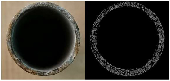
Figure 1.
Canny Algorithm detection effect.
Figure 1 highlights that the edge map that was extracted by the canny operator has many cluttered edges that affect the measuring of the building steel pipe size. Although the traditional image processing methods are more mature, practical applications require a variety of pre-processing that is applied to the original image. However, the pre-processing strategy is heavily affected based on the actual situation and is not uniform. Moreover, the edge detection operator also suffers from adjusting its parameters. Furthermore, the real scene is more complex in engineering, and the detected objects have different degrees of wear, damage, and other influencing factors. Therefore, the traditional methods do not pose a practical solution, as these are easily disturbed and are less robust. With the advancement of machine learning research, automatically extracting the image features has become a reality. Several neural networks [13] and support vector machines [14] have already been introduced to replace manual feature extraction in edge detection. Further development in machine learning and deep learning, especially the convolutional neural networks, can extract more complex image features, presenting a practical solution compared to traditional image processing methods.
1.2.2. Background of Convolutional Neural Networks
In recent years, many algorithms have achieved an appealing performance with the rise of artificial intelligence and especially the development of convolutional neural networks (CNNs). For instance, [15] combines a CNN with the nearest neighbor search, where the former calculates the features of each patch in the image, and then the latter searches in the dictionary to find similar edges, to finally integrate the edge information and output the result. In [16], the authors use depth features that are learned by a CNN to improve the edge detection accuracy. In 2015, Xie et al. [17] proposed the HED (holistically-nested network) edge detection model, where edge information extraction using convolutional neural networks has become one of the many hot research topics. The HED model involves a side-output network framework for edge detection by considering feature fusion in the convolutional layer using the deep supervision structure without increasing the depth of the backbone network. In 2016, Yu Liu et al. introduced the RDS (relaxed deep supervision) edge detection method based on deep convolutional neural networks at the CVPR (IEEE Conference on Computer Vision and Pattern Recognition) Computer Vision Topical Conference [18]. The innovation of this algorithm is utilizing relaxed labels to solve the problem of whether a pixel in an image is an edge point or not. In 2018, Liu proposed the RCF algorithm [19], which fully exploits the feature information from each convolutional layer and surpasses even the recognition ability of the human eye in terms of detection accuracy. A context-aware deep edge detection tracking strategy has also been proposed [20]. In [21], the authors suggest a new multiscale approach to constructing down-sampling pyramid networks and lightweight up-sampling pyramid-rich encoders and decoders. From the development of edge detection technology, it is evident that with the development of deep learning technology, the edge detection algorithms that are based on CNNs surpass the traditional edge detection operators. Moreover, based on the image processing capability of CNNs, features can be extracted effectively without processing the original image. Therefore, this paper performs image processing based on edge information that is extracted from a CNN, affording high-accuracy detection results. In practical engineering, there are many cases of wear and damage at the cross-section of the construction steel pipe. In this case, compared with the RCF network, the ODS and OIS of the proposed network model are increased by 3% and 2.2%, respectively.
The image can be obtained as a coarse edge image after edge detection, and the rough edge image of the building steel pipe is circular. The circle detection algorithm generally includes a random Hough transform, random sample consistency, and random circle detection. The work of [22] proposes a fast and accurate random circle detection algorithm to obtain higher detection speeds and accuracy. In [23], the authors suggest a method that is based on central clustering to identify rod-subjected particles, which combines K-means and DBSCAN algorithms that are used to detect circles. A new model combining a complete variation algorithm with an improved Hough transform is proposed in [24] to extract the edges of annual wood rings. Ref. [25] uses the Hough detection algorithm to locate holes, effectively identifying spots. The connected domain labeling algorithm is introduced in [26,27], which can find various shapes quickly. In this work, we reasonably employ the connected domain properties and combine them with the Hough circle detection algorithm to propose an optimized Hough circle detection scheme. In this paper, the improved Hough circle detection method presents a lower error than the classic Hough circle detection scheme, obtaining an accurate result. The flow chart of this paper is illustrated in Figure 2.
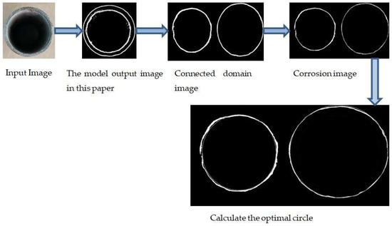
Figure 2.
Flowchart of the Hough circle detection method.
2. Network Model
Convolutional neural networks have strong feature learning abilities and can learn high-order features in images. HED and RCF, as classic deep learning algorithms in edge detection, have achieved appealing results. In this paper, the edge features of construction steel pipes are extracted based on the improved RCF network, and then the feature images are processed.
When applying machine vision for size measurement, the edge extraction of the object is an essential part. By extracting the edge image of an object and then converting the pixel space in the edge image into the actual physical distance using pixel equivalence, the actual size of an object can be measured. The development of the traditional edge detection operators has been relatively mature and straightforward but has certain limitations in the actual application environment. In practical applications, the edges of architectural steel pipes are subject to multiple wear and tear, and the cross-sectional information is rather messy. These effects cannot be circumvented using the traditional edge detection operator, and the detection is ineffective.
Through the above analysis, the edge detection algorithm of this paper is requested to explore an edge detection method that is applicable to construction projects, which makes the cluttered texture features of the cross-section of the construction steel pipe less influential and outputs only the desired edge information. Hence, we propose an improved RCF coarse edge detection that uses a CNN to extract the image’s edge features, which does not need to pre-process the original image. Additionally, to accurately measure the dimensions of the cross-section of the building steel pipe, the extracted rough edge images are processed to obtain more accurate edge dimensions.
2.1. Improved RCF-Based Coarse Edge Detection Method
RCF is based on the VGG16 network and realizes end-to-end edge detection. The network structure of RCF is divided into three parts: backbone network, deep supervision module, and feature fusion module. The backbone network uses the fully convolutional layer of VGG16, realizing the automatic extraction of edge features. The deep supervision module performs supervised learning on each stage to output an edge image. The feature fusion module uses a 1 × 1 convolutional layer to fuse the feature maps that are generated by each stage and finally outputs the fused feature image. The features that are extracted by the convolutional neural network in various depth layers differ, and the underlying network learns simple location information. With the increase of the level depth, the high-level network structure abstractly integrates the basic features thata re learned by the underlying network, the location information is continuously lost, and the semantic information in the image is constantly enriched. The network structure of the model has low-level and high-level information to ensure the quality of the edge image.
- Algorithm design
The RCF network model is generalized based on the improved edge detection HED model. The RCF network model extracts more complete edge features with a less interfered contour, and the robustness is enhanced. However, directly using RCF for the edge extraction of architectural steel pipe suffers from edge blurring, and the contour is interfered. The reason is mainly due to the CNN’s characteristics, as after undergoing multiple convolutions, many details of the image feature information are lost. To overcome this problem, this paper adopts the following improvements:
- (1)
- The proposed model uses the dil (dilation convolution) module in the last stage, which adds voids to the standard convolution layer to increase the perceptual field. Compared with standard convolution, the dilation convolution has one more dilation parameter, which in this work is set to 2.
- (2)
- In the RCF model, a loss calculation function is added at the end of each stage, and a deconvolution layer is upsampled in each layer to map the image size to the original size. Finally, the output of each stage is superimposed on a 1 × 1 − 1 convolution to merge multiple channels and calculate the loss. Our model only uses it for loss calculation of the images after merging multiple channels, affording our model to detect edges more clearly and interfere with fewer contour lines than the original model. The network model of this paper is illustrated in Figure 3.
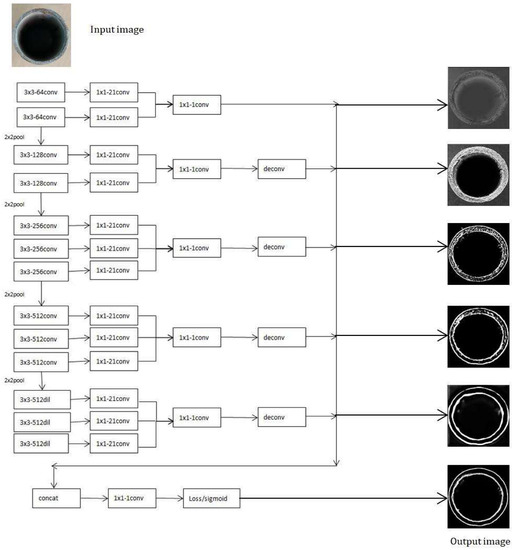 Figure 3. Network model in this paper.
- Training sample set
We created our training set for image edge detection of building steel pipes for the application scenario that was investigated. Data enhancement is performed on the collected dataset, which is expanded by rotating, mirroring, and deflating the 100 initial data to 400 training sets and 50 test sets. The Labelme tool is used to manually label the edges in the training set and the edge features that are learned by the training model are used to adjust the network parameters to make the output match the expected value and obtain a clearer edge image. Figure 4 depicts the collected dataset and the manually labeled edge images.
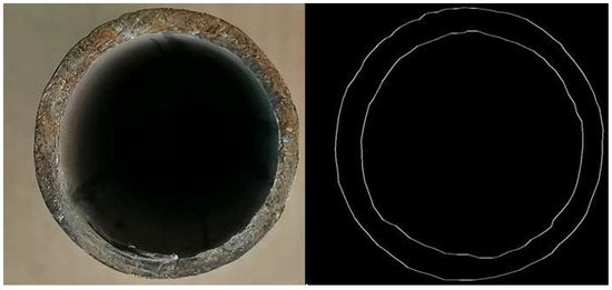
Figure 4.
Making a dataset.
2.2. Model Training and Detection
The experiments were conducted on a Windows operating system using Pytorch as the development framework, with an NVIDIA Tesla P100- PCI-E-16GB graphics card and Cuda version 11.2. The Labelme tool was used to mark the edges.
In this paper, the CNN that was used is the RCF model. The loss must calculate each layer of the feature image in the original model and the fused feature image. This training method does not reflect the importance of the fused feature image and the edge images of each stage on the network model to optimize the model better. The fused feature image is the final output image, with the model neglecting the loss calculation of the deep supervision module and only using the fused loss for training. The following parameters of the VGG16 model are used as the initial values to train the model.
- (1)
- Choice of the loss function
For the edge detection problem, which is a binary classification problem of pixel points, i.e., edge points or non-edge points, the edge detection dataset is usually marked by multiple markers. For each image marker, an edge probability map is generated, ranging from zero to one, where zero means there is no marker at the pixel and one means the quality is marked at this pixel. The pixel with an edge probability that is higher than η is considered a positive sample, while pixels with a chance that is equal to zero are considered negative samples. If a pixel point is marked by a marker that is less than η, it is considered a disputed point, and treating the disputed issue will confuse the network, so the model directly ignores the disputed issue. For the binary classification problem of pixel points, this model uses the cross-entropy function as the loss function and calculates the loss function of each pixel point expressed as:
where Y+ and Y− represent the number of positive and negative samples, the hyperparameter λ is used to balance the difference between the number of positive and negative examples, Xi is the activation value of the neural network, Yi is the probability value that pixel i is an edge point in the labeled graph, and W represents the parameters that can be learned in the neural network. After removing the loss calculation of the deep supervision module, the loss formula for each picture is:
- (2)
- Backward propagation parameters and activation functions
The backpropagation algorithm uses an SGD optimization algorithm, and the base learning rate is kept constant during the training process. The base learning rate is set to 1 × 10⁻⁷, and the specific parameters are adjusted according to the actual sample situation. The sigmoid function is used for the activation function. For the binary classification problem, the sigmoid function can transform the input arbitrary value x into a value between 0 and 1 to achieve data mapping. The formula is as follows:
- (3)
- Training process
During the training process, the value of loss represents the pixel error between the edge images thata re generated by the network model and the manually annotated map, which can visually observe the good or bad training results. Figure 5 (left) shows the loss value curves during the training of the RCF network model, and the figure on the right represents the loss value curve of the network model that is suggested in this paper. The figure highlights that the value of the loss function decreases with the growth of the training number. Moreover, the curve is smoother than the original curve, and the loss curve gradually converges when the training set is iterated for a certain number of times, indicating that the edge images that are generated by the network model are gradually approaching the manually labeled edge images.
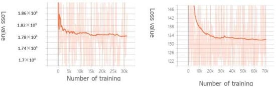
Figure 5.
Loss value change.
The detection model is trained for 650 iterations, with Figure 6 depicting the image input into the detection model. Specifically, the left image in Figure 6 is the test result of the original RCF network model, which presents some confusing and unclear edge lines. Part of the edge lines are intermittent and cannot be used to measure the cross-section of the building steel pipe. However, Figure 6 (right) illustrates our model’s output highlighting its effectiveness compared to the original model, affording clearer and more realistic lines without messy details and continuous edge lines. After removing the loss calculation of the deep supervision module, the time to calculate the loss of six pictures becomes the time to calculate the loss of one image. The time complexity changes from T(6) to T(1), the space storage of six images becomes the space storage of one image, and the space complexity changes from O(6mn) to O(mn), significantly reducing the running time and space storage.
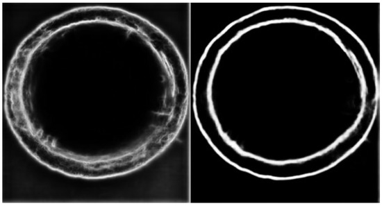
Figure 6.
Comparison of the test results.
2.3. Experimental Analysis
The evaluation metrics of edge detection models are mainly the ODS (optimal dataset scale) and OIS (optimal image scale). ODS refers to the detection results when a uniform threshold is used for all images in the test set, and OIS is the detection result when using the best threshold for the currently available image. This paper measures the indicators using the Matlab tool. Table 1 compares each indicator with the Canny operator and RCF, revealing that in this paper’s dataset, our model attains a better performance than RCF. Indeed, our model’s ODS and OIS are 3% and 2.2% higher than RCF, respectively.

Table 1.
The model is compared with the RCF results.
3. Image Processing of Coarse Edges
The image that was obtained from the improved RCF-based algorithm is clearer, the edge contour is complete, and the interference contour line is less. To improve the edge detection accuracy, we process the coarse edge images by applying corrosion operation, connected domain, and circle detection for binary images.
3.1. Connected Domain-Based Image Processing
The connected region generally refers to the image area with the same pixels and adjacent pixel points in a position. The binary image after the above processing is subjected to the connected domain labeling algorithm, which is divided into two pictures of different domains. This strategy affords not disturbing the exact center and radius of one circle by another area. The labeling algorithms for the connected parts can be broadly classified into three methods: line labeling, pixel labeling, and region growing.
The connected domain-based image processing algorithm calls the cv2.connectedComponentsWithStats function in Python when implementing the connected domain distinction. This function returns the number of all connected domains, the marker for each pixel in the image, the statistics for each title, and the centroid of the connected part. During the implementation, it was found that our dataset may have some independent points or lines in the binary image after processing and background information in the picture so that some abnormally connected domains will be detected. By appropriately setting the threshold value of the connected domains, the irregular connected domains and the background information of the image are discarded, removing the error information due to the abnormally connected domains and leaving two correctly connected domains, as depicted below.
Figure 7 shows the image without connected domain. As shown in Figure 8, by using connected domains, the contour lines in the image are rougher, imposing a significant error on the refined size detection. To reduce this error, we exploit the binary image etching operation, and specifically the contour line etching. The etching effect is illustrated in Figure 9.
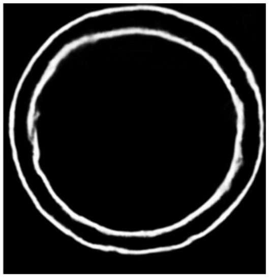
Figure 7.
Diagram of the unrealized connected domains.
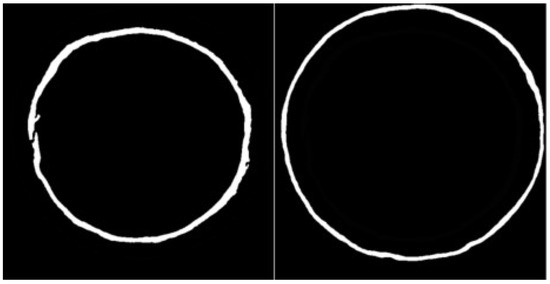
Figure 8.
After realizing the connectivity domain.
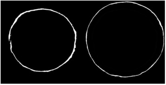
Figure 9.
Image after corrosion.
3.2. Accuracy of Circle Detection Based on Hough Transform
3.2.1. Hough Circle Detection
The principle of the Hough transform circle detection: Assuming that the circle’s radius is r0 and the coordinates of the center are (a0, b0), a circle is expressed as in (6). Projecting any point (xi, yi) of the circle into the parameter space is realized through expression (7). If a, b, and rare are the three variables in the parameter space and (xi, yi) corresponds to any point of the circle in the original image, which are all known, then Equation (7) is a circle in the parameter space. As r grows step-wise between [rmin and rmax], the expression of any point in space can be expressed as a conic surface. With the increase in (xi, yi), numerous conic surfaces will be formed in the parameter space. However, the conic surfaces must intersect at a point (a0, b0). This point is the center of the circle of the original image, as shown in Figure 10.
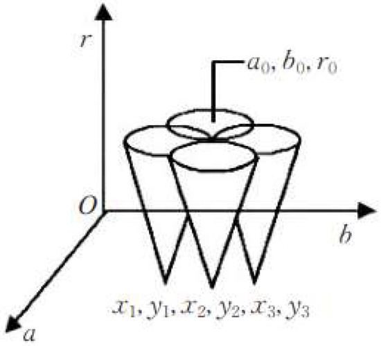
Figure 10.
Hough diagram.
3.2.2. Radius Circle Centering Accuracy
This paper applies the advantages of Hough circle detection for localizing the initial circle. The process of dealing with the radius in this paper relies on the equal distance from the point on the circle to the center of the circle to find the value of the radius according to the specificity of the graphical data. During the experiment, it was found that the Hough circle detection could not detect concentric circles, and the parameters needed to be adjusted each time a curve was detected in the graph, which was overly burdensome. Based on the image of the above-connected domain and the Hough circle detection, the circle in the chart can be detected by adjusting the parameters only once during the experiment. The detection effect can be positioned to the pixel level of the center and the circle’s radius, also affording better robustness. In this paper, we optimize the accuracy aspects of the radius and the center of a circle in the graph based on the connected-domain Hough circle detection, as follows:
- (1)
- Using the image of the connected domain, the approximate circle center, and coordinates of the circle in the picture are first detected using Hough circle detection.
- (2)
- Then, we determine the 8-neighborhood of the circle center based on the circle center that is found, and use the 8-neighborhood as the error circle center.
- (3)
- We calculate the distance from all the points on the image to the center of the eight circles and take the average as the radius.
- (4)
- We draw eight circles that are centered at the eight neighborhoods and the radius that is calculated in the previous step. Then, we calculate the overlap between these nine standard circles and the graph. The circle with the highest degree of overlap is the optimal circle.
The algorithm flow is shown in Figure 11:
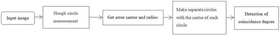
Figure 11.
Algorithm flow chart.
In Figure 12, the top four circles are the outcome of using Hough circle detection, and the following circles (including the results of Hough circle detection) compare the overlap to define the impact of the optimal circle. The following figure compares these findings in detail.
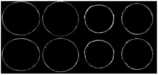
Figure 12.
Comparison of the results.
In Figure 13, the left side illustrates the edge detail of the Hough circle detection, and the right side is the edge detail with the highest overlap. After optimizing the proposed algorithm, it can be seen that the detected circle fits the circle in the graph to a greater extent. By achieving the circle pixel overlap, the line width of each circle is the same, not affecting the results by the line width. Table 2 compares the number of pixel overlaps per circle.
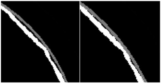
Figure 13.
Detail comparison.
Table 2.
Pixel consistency comparison.
The images that were used in this article are all 72 dpi. The circle’s radius (number of pixels per unit) is obtained from the following equation. We convert the number of pixels into centimeters using the following formula:
where C is the radius in centimeters, P is the number of pixels, and R is the resolution. The measured values were obtained with an image measuring tool. Next, we compare the proposed algorithm, Hough circle detection, and manual measurement against the true radius of the steel pipe (unit centimeter). As shown in Table 3.
Table 3.
Radius of contrast.
The experiments show that the Hough circle detection algorithm is very close to the true circle, and the edge line is very thin with some anomalies in a few cases, while the detection effect is good. However, in the case of thick edge lines and irregular circles, the Hough circle detection is affected by the irregular edges and is shifted to one side. In the case of practical applications, the cross-section of the construction steel pipe is subject to damage, wear, and other conditions. Thus, solely employing Hough circle detection is not a suitable method. In contrast, the improved algorithm retains Hough circle detection’s advantages but also improves the detection accuracy.
3.3. Error Analysis
The errors in the images that are created using the suggested method are as follows.
- Image clarity. Using CNNs does not require pre-processing the image and affords better robustness. However, to a certain extent, image clarity still impacts the extraction of coarse edges.
- Algorithm error. The coarse edge that is obtained by the optimized RCF model and binary image erosion, although as close as possible to the actual edge, still cannot accurately locate the actual edge.
4. Conclusions and Outlook
4.1. Summary
Currently, the construction engineering measurement of steel pipe size is a slow process that is not accurate. Therefore, this paper utilizes deep learning and image processing technology to improve the existing technology and solves the issues of slow speed and poor accuracy during manual measurements. The main innovations of this paper are as follows:
- A dimensional detection method for architectural steel tubes is proposed, which utilizes convolutional neural networks to extract edge features, solving the problem of the poor robustness of the traditional edge detection operator and improving practicality.
- Based on the problem of coarse edge size detection, this paper proposes an optimization algorithm for Hough circle detection based on the connected domain and binary image processing, making the Hough circle detection algorithm more applicable to engineering.
4.2. Outlook
This paper considers the environmental problems in real engineering and specifically investigates visual inspection technology for damaged and not easily detectable construction steel pipes. Future improvements shall involve:
- Optimize the coarse edge extraction model further so that the coarse edge image can be free of interference edge lines. This will improve the image processing rate and, thus, the speed of visual detection.
- Optimizing the fine edge algorithm based on coarse edge extraction to reduce the error between the refined edge and the actual edge.
- In this paper, only the cross-section size of the steel pipe is measured, and the length of the steel pipe can be further calculated using edge detection technology.
- Extending this technology to measure circular objects.
Author Contributions
Conceptualization, F.Y.; Formal analysis, Z.Q.; Investigation, Z.Q.; Methodology, R.L.; Project administration, Z.J.; Supervision, F.Y.; Validation, Z.Q.; writing—original draft, F.Y.; writing—review and editing, F.Y. and Z.Q. All authors have read and agreed to the published version of the manuscript.
Funding
This publication has emanated from a research conducted with the financial support of the National Key Research and Development Program of China under the Grant No. 2017YFE0135700.
Conflicts of Interest
The authors declare no conflict of interest.
References
- Cerruto, E.; Manetto, G.; Privitera, S.; Papa, R.; Longo, D. Effect of Image Segmentation Thresholding on Droplet Size Measurement. Agronomy 2022, 12, 1677. [Google Scholar] [CrossRef]
- Al-Haija, Q.A.; Gharaibeh, M.; Odeh, A. Detection in Adverse Weather Conditions for Autonomous Vehicles via Deep Learning. AI 2022, 3, 303–317. [Google Scholar] [CrossRef]
- Cavedo, F.; Norgia, M.; Pesatori, A.; Solari, G.E. Steel pipe measurement system based on laser rangefinder. IEEE Trans. Instrum. Meas. 2016, 65, 1472–1477. [Google Scholar] [CrossRef]
- Xin, R.; Zhang, J.; Shao, Y. Complex network classification with convolutional neural network. Tsinghua Sci. Technol. 2020, 25, 447–457. [Google Scholar] [CrossRef]
- Yang, J.; Yu, W.; Fang, H.-Y.; Huang, X.-Y.; Chen, S.-J. Detection of size of manufactured sand particles based on digital image processing. PLoS ONE 2018, 13, e0206135. [Google Scholar] [CrossRef] [PubMed]
- Rong, X.; Liao, Y.; Jiang, L. Size Measurement Based on Micro-Irregular Components. Sci. J. Intell. Syst. Res. 2021, 3. [Google Scholar]
- Kong, R. Machine Vision-based Measurement System of Rubber Hose Size. J. Image Signal Process. 2021, 10, 135–145. [Google Scholar] [CrossRef]
- Zhang, L.; Yang, Q.; Sun, Q.; Feng, D.; Zhao, Y. Research on the size of mechanical parts based on image recognition. J. Vis. Commun. Image Represent. 2019, 59, 425–432. [Google Scholar] [CrossRef]
- Yu, W.; Zhu, X.; Mao, Z.; Liu, W. The Research on the Measurement System of Target Dimension Based on Digital Image. J. Phys. Conf. Ser. 2021, 1865, 042072. [Google Scholar] [CrossRef]
- Huang, Y.; Ye, Q.; Hao, M.; Jiao, J. Dimension Measuring System of Round Parts Based on Machine Vision. In Proceedings of the International Conference on Leading Edge Manufacturing in 21st Century, LEM21, Fukuoka, Japan, 7–9 November 2007; Volume 4, p. 9E532. [Google Scholar]
- Xu, Z.; Ji, X.; Wang, M.; Sun, X. Edge detection algorithm of medical image based on canny operator. J. Phys. Conf. Ser. 2021, 1955, 012080. [Google Scholar] [CrossRef]
- Hao, F.; Xu, D.; Chen, D.; Hu, Y.; Zhu, C. Sobel operator enhancement based on eight-directional convolution and entropy. Int. J. Inf. Technol. 2021, 13, 1823–1828. [Google Scholar] [CrossRef]
- Paik, J.K.; Katsaggelos, A.K. Edge detection using a neural network. In Proceedings of the International Conference on Acoustics, Speech, and Signal Processing, IEEE, Albuquerque, NM, USA, 3–6 April 1990; pp. 2145–2148. [Google Scholar]
- Meng, F.; Lin, W.; Wang, Z. Space edge detection based SVM algorithm. In Proceedings of the International Conference on Artificial Intelligence and Computational Intelligence, Taiyuan, China, 24–25 September 2011; Springer: Berlin/Heidelberg, Germany, 2011; pp. 656–663. [Google Scholar]
- Ganin, Y.; Lempitsky, V. N4-Fields: Neural Network Nearest Neighbor Fields for Image Transforms. In Proceedings of the Asian Conference on Computer Vision, Singapore, 1–5 November 2014; Springer: Cham, Switzerland, 2014; pp. 536–551. [Google Scholar]
- Shen, W.; Wang, X.; Wang, Y.; Bai, X.; Zhang, Z. A deep convolutional feature learned by positive-sharing loss for contour detection. In Proceedings of the IEEE Conference on Computer Vision and Pattern Recognition, Boston, MA, USA, 7–12 June 2015; pp. 3982–3991. [Google Scholar]
- Xie, S.; Tu, Z. Holistically-nested edge detection. In Proceedings of the IEEE International Conference on Computer Vision, Santiago, Chile, 7–13 December 2015; pp. 1395–1403. [Google Scholar]
- Liu, Y.; Lew, M.S. Learning relaxed deep supervision for better edge detection. In Proceedings of the IEEE Conference on Computer Vision and Pattern Recognition, Las Vegas, NV, USA, 27–30 June 2016; pp. 231–240. [Google Scholar]
- Liu, Y.; Cheng, M.M.; Hu, X.; Wang, K.; Bai, X. Richer Convolutional Features for Edge Detection. In Proceedings of the IEEE Conference on Computer Vision and Pattern Recognition, Honolulu, HI, USA, 21–26 July 2017; pp. 3000–3009. [Google Scholar]
- Huan, L.; Xue, N.; Zheng, X.; He, W.; Gong, J.; Xia, G. Unmixing Convolutional Features for Crisp Edge Detection. IEEE Trans. Pattern Anal. Mach. Intell. 2021, 44, 6602–6609. [Google Scholar] [CrossRef] [PubMed]
- Li, K.; Tian, Y.; Wang, B.; Qi, Z.; Wang, Q. Bi-Directional Pyramid Network for Edge Detection. Electronics 2021, 10, 329. [Google Scholar] [CrossRef]
- Jiang, L. A fast and accurate circle detection algorithm based on random sampling. Future Gener. Comput. Syst. 2021, 123, 245–256. [Google Scholar] [CrossRef]
- Scitovski, R.; Sabo, K. A combination of k -means and DBSCAN algorithm for solving the multiple generalized circle detection problems. Adv. Data Anal. Classif. 2021, 15, 83–98. [Google Scholar] [CrossRef]
- Du, W.; Xi, Y.; Harada, K.; Zhang, Y.; Nagashima, K.; Qiao, Z. Improved Hough Transform and Total Variation Algorithms for Features Extraction of Wood. Forests 2021, 12, 466. [Google Scholar] [CrossRef]
- Liang, Y.; Zhang, D.; Nian, P.; Liang, X. Research on the application of binary-like coding and Hough circle detection technology in PCB traceability system. J. Ambient. Intell. Humaniz. Comput. 2021, 1–11. [Google Scholar] [CrossRef]
- Miao, H.; Teng, Z.; Kang, C.; Muhammadhaji, A. Stability analysis of a virus infection model with humoral immunity response and two time delays. Math. Methods Appl. Sci. 2016, 39, 3434–3449. [Google Scholar] [CrossRef]
- Zhang, F.; Li, J.; Zheng, C.; Wang, L. Dynamics of an HBV/HCV infection model with intracellular delay and cell proliferation. Commun. Nonlinear Sci. Numer. Simul. 2017, 42, 464–476. [Google Scholar] [CrossRef]
Publisher’s Note: MDPI stays neutral with regard to jurisdictional claims in published maps and institutional affiliations. |
© 2022 by the authors. Licensee MDPI, Basel, Switzerland. This article is an open access article distributed under the terms and conditions of the Creative Commons Attribution (CC BY) license (https://creativecommons.org/licenses/by/4.0/).