Joint Semantic Intelligent Detection of Vehicle Color under Rainy Conditions

Abstract

Color is an important feature of vehicles, and it plays a key role in intelligent traffic management and criminal investigation. Existing algorithms for vehicle color recognition are typically trained on data under good weather conditions and have poor robustness for outdoor visual tasks. Fine vehicle color recognition under rainy conditions is still a challenging problem. In this paper, an algorithm for jointly deraining and recognizing vehicle color, ($JADAR$), is proposed, where three layers of $UNet$ are embedded into $RetinaNet\text{-}50$ to obtain joint semantic fusion information. More precisely, the $UNet$ subnet is used for deraining, and the feature maps of the recovered clean image and the extracted feature maps of the input image are cascaded into the Feature Pyramid Net ($FPN$) module to achieve joint semantic learning. The joint feature maps are then fed into the class and box subnets to classify and locate objects. The $RainVehicleColor\text{-}24$ dataset is used to train the $JADAR$ for vehicle color recognition under rainy conditions, and extensive experiments are conducted. Since the deraining and detecting modules share the feature extraction layers, our algorithm maintains the test time of $RetinaNet\text{-}50$ while improving its robustness. Testing on self-built and public real datasets, the mean average precision ($mAP$) of vehicle color recognition reaches $72.07\%$, which beats both sate-of-the-art algorithms for vehicle color recognition and popular target detection algorithms.

1. Introduction

Vehicle information recognition has been applied in the field of intelligent traffic management and criminal investigation. License plate, model, and vehicle color comprise the main vehicle information. Although license plate recognition is a commonly used vehicle information recognition technology [1], it also faces many challenges in criminal investigation and for intelligent traffic law enforcement, as license plates can be easily obscured (partially or fully) or faked/duplicated by criminals. As it can still be identified despite partial occlusion or viewpoint changes, vehicle color recognition is widely applied in video surveillance [2], vehicle detection [3], vehicle tracking [4], automatic driving [5,6], criminal investigation [7], etc. All the above-mentioned tasks inevitably encounter adverse weather conditions, especially rain. This, in turn, adversely affects the performance of object recognition/retrieval, because rain can significantly reduce the contrast of the scene and reduces visibility, compromising image quality. Many scholars have conducted research on how to improve the performance of object detection under rainy conditions.

Vehicle color recognition methods are typically classified as traditional model-driven [8,9,10,11] or data-driven deep learning [12,13,14,15,16,17,18]. Traditional methods usually use handcrafted feature descriptors to extract visual features and train a classifier to recognize vehicle color. For example, Chen et al. [8] select the region of interest (ROI) of the vehicle to recognize its dominant color and than train a linear support vector machine to classify it. Jeong et al. [9] adopt $AdaBoost$ to classify an $HSV$ histogram of the vehicle’s homogeneity patches into seven color categories.

Deep neural networks have been employed to learn effective feature representations from raw pixels, which has proven to be more powerful than traditional methods. To be more specific, these deep learning methods fall into two groups: general object detection algorithms [19,20,21,22,23,24] applied to vehicle color recognition [16,17,18] and algorithms specially designed for color recognition. All these algorithms are trained on datasets with 7–24 colors [8,9,10,18] obtained under normal weather conditions. Of course, there exists some research to address object recognition under rainy conditions; basically, these proposed methods adopt two-stage instead of end-to-end procedures, which inevitably increases the running time of the entire task.

On the other hand, a number of scholars have paid attention to joint processing of low-level and high-level tasks. Generally, they improve the robustness of object detection [25,26,27,28] by embedding domain adaptation, image restoration, style transfer, or other modules into the object detection framework, or by a few-shot transfer learning mechanism [29,30,31,32]. These methods have explored the robustness of performance for downstream tasks in many harsh environments except under rainy weather conditions, which motivated our work in the present paper.

In this paper, a Joint Algorithm for Deraining And Recognition (JADAR) is proposed for fine recognition of vehicle color under rainy conditions. The network architecture is shown in Figure 1. To be more specific, we embed the three-layer decoder of $UNet\text{-}3$ into the last three layers of the feature extraction submodule of $RetinaNet\text{-}50$. The main contributions are as follows:

• $JADAR$ contains far fewer parameters than previous two-stage methods since its subnets, $UNET$ and $RetinaNet$ share the same feature extracting layers. This is of high practical value as the size of outdoor mobile equipment can be substantially reduced.
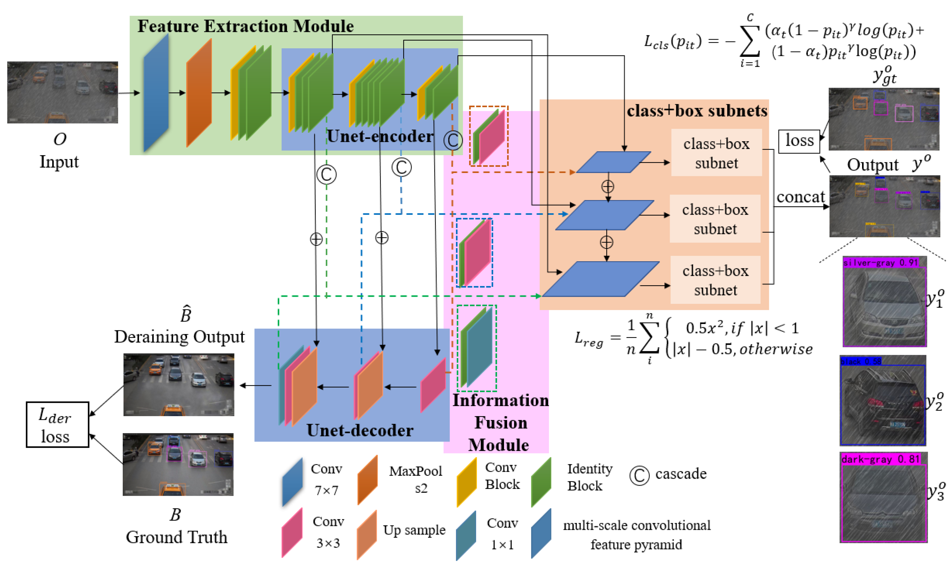
• In $JADAR$, the multi-scale fusion information obtained by cascading feature maps of original rainy images and recovered images are fed into the subsequent class-box subnet. In so doing, multi-scale information across domains is crucially beneficial for fine vehicle color recognition.
• The joint processing of low-level and high-level tasks can be mutually beneficial. Embedding the image restoration module can help improve the performance of subsequent high-level tasks under severe weather; conversely, the performance of subsequent high-level tasks as evaluation metrics can, in turn, fine-tune the image restoration algorithms.
• Comprehensive experiments show that our proposed methods outperform basic detection networks and two-stage network and transfer learning methods for the task of color recognition under rainy conditions. Further, our training and testing times are shortened.

Next, related work is introduced in Section 2. $JADAR$ is constructed in Section 3. Section 4 shows that our method is superior to the state-of-the-art quantitatively and qualitatively. Section 5 concludes the main content.

2. Related Work

There exists some research on vehicle color recognition under normal weather and object detection under adverse weather conditions, which is reviewed below.

2.1. Vehicle Color Recognition under Normal Weather Conditions

Vehicle color recognition methods generally fall into traditional model-based methods [8,9,10,11] and data-based deep learning methods [12,13,14,15,16,17,18]. Regarding traditional model-based methods, Chen et al. [8] train a linear support vector machine classifier on the region of interest $ROI$ in vehicle images based on eight color types; Jeong et al. [9] adopt the multi-class AdaBoost algorithm to classify the color of front-of-vehicle images into seven types; Dule et al. [11] train three classifiers (KNN, ANN, and SVM) for two $ROI$s (smooth hood section and semi-front of vehicle).

Data-based methods have been receiving increasing attention for vehicle color recognition. Hu et al. [12] were the first to apply a convolutional neural network (CNN) with a spatial pyramid strategy to boost the accuracy of vehicle color recognition. Zhang et al. [15] proposed a lightweight $CNN$ for vehicle color recognition. Fu et al. [16] designed $MCFF\text{-}CNN$ (Multiscale Comprehensive Feature Fusion Convolutional Neural Network) to recognize eight vehicle colors. Hu et al. [18] proposed vehicle color recognition based on a Smooth Modulation Neural Network with Multi-Scale Feature Fusion ($SMNN\text{-}MSFF$).

It is worth mentioning that there has been no research on vehicle color detection under bad weather conditions, which is the focus of this paper.

2.2. Object Detection under Adverse Weather Conditions

Bad weather includes rain, snow, haze, etc. The quality of outdoor images or videos collected in these weathers is severely degraded, so target-detection models trained on high-quality images have difficulty handling bad weather. This challenge has been investigated by many scholars with many solutions provided, such as embedding a domain-adaptation module [25,26,27,28,31,33,34] into the object detection backbone, such as $YOLO$, $Faster$$RCNN$, $RetinaNet$, etc., two-stages methods consisting of preprocessing and object detection [35,36,37,38,39,40], or using a few-shot transfer learning mechanism [29,30,31,32].

For example, Chen et al. [33] embedded two domain adaptation modules into $Faster$$RCNN$ to reduce the domain discrepancy on image level and instance level. Sindagi et al. [31] proposed an unsupervised domain-adapting method to improve generalization of object detection under hazy and rainy conditions. Style transfer is considered in [27], in which the authors construct a cross-domain representation learning method including domain diversification and a multi-domain invariant. Huang et al. [41] combine dual subnet frameworks for object detection under foggy conditions.

Except for the two-stage methods, the above-mentioned methods do not pay special attention to the rainy conditions. However, two-stage methods such as [35,36,37,38,39,42] do pay attention to image deraining instead of object detection. in other words, the joint tasks of deraining and object detection are not taken seriously. Motivated by the above considerations, we propose $JADAR$ for joint semantic intelligent detection of vehicle color in rainy scenes.

3. JADAR Algorithm

3.1. Fusion Network Design

In this paper, a Joint Algorithm for Deraining And Recognition (JADAR) is designed for vehicle color recognition in inclement weather conditions; it is based on $RetinaNet\text{-}50$, as shown in Figure 1. In Figure 1, O is the rainy image input, B is the corresponding clean background image, $\widehat{B}$ and $y^o$, respectively, are the outputs of the deraining and detecting results. To see results clearly, we zoom in on the recognition results of each car in picture $y_i^o(i=1,2,3)$; $y_1^o$ is the enlarged result of the first car in the picture—the recognition color is silver-gray with a confidence level of $0.91$; $y_2^o$ is the enlarged result of the second car in the picture—the recognition color is black with a confidence level of 0.58; $y_3^o$ is the enlarged result of the third car in the picture—the recognition color is dark gray with a confidence level of $0.81$. The green/blue/purple/orange boxes represent the feature extraction module/UNet-3/ information fusion module/class+bbox subnets, respectively. $L_{reg}$ is the regression loss using the smooth L1 loss. $L_{cls}$ is the classification loss using the focal loss. The loss function for deraining is MSE loss. $JADAR$ is trained by the weighted sum of these three losses (see Equation (7)).

The $JADAR$ framework is designed by embedding the three-layer decoder of UNet-3 [43] into the last three sub-blocks of the feature extraction module, as illustrated by the green-tinted box in Figure 1. The whole framework consists of four main modules: image feature extraction module, deraining module, information fusion module, and $class+box$ subnets. The rain removal and feature extraction modules share three layers, avoiding extra computational burden. In fact, Section 4.5 shows that $JADAR$ has the same testing time as $RetinaNet\text{-}50$. The last three feature maps and the corresponding recovered feature maps are cascaded together and then fed into their respective $class+box$ subnets, which can learn multi-scale joint semantic representations to improve object detection accuracy under rainy conditions. The feature fusion sub-module setting is illustrated in Figure 2.

The overall object function is back-propagated to train the deraining module and to improve rainy image deraining performance recursively. The object detection backbone network uses three-scale $class+box$ subnets to leverage multi-scale fusion color feature maps to classify 24 car color types and locate the bounding-box.

3.2. Model Formulation and Model Optimization

Let the physical mechanism of rainy image corruption be

$$x=y+z$$

(1)

where $x,y,z$ denote rainy image O, recovered clean background image B, and rain layer R, respectively. To tackle the problem of supervised vehicle object detection by color in inclement weather conditions, a joint network is proposed to learn joint semantic representation from an input rainy image x. Let y denote the corresponding label of rainy image x.

As demonstrated by the green box in Figure 1, the last three feature maps $f_1\left(x\right)$, $f_2\left(x\right)$, $f_3\left(x\right)$ are taken from the feature extraction sub-blocks of $RetinaNet$. Then, $f_1\left(x\right)$ is fed into the corresponding last layer of the decoder of $UNet$-3, and $g_1\left(x\right)$ is output. Next, $g_1\left(x\right)$ and $f_2\left(x\right)$ are cascaded into the penultimate layer $UNet$-3, and $g_2\left(x\right)$ is output; then $g_2\left(x\right)$ and $f_3\left(x\right)$ are cascaded into the last decoder layer of $UNet$-3, and $g_3\left(x\right)$ is output. The output of the deraining module $\widehat{y}$ is denoted by $g_3\left(x\right)$. Thus, the mean square error ($MSE$ loss) is used as deraining object function $L_{der}$ as follows:

$$L_{der}=\frac{1}{n}\sum _{i=1}^n{\parallel (\widehat{y}-y)\parallel }^2$$

(2)

where n is the number of rainy images. Finally, $f_1\left(x\right)$ and $g_1\left(x\right)$, $f_2\left(x\right)$ and $g_2\left(x\right)$, and $f_3\left(x\right)$ and $g_3\left(x\right)$ are cascaded and input into differently scaled $class+box$ subnets, where joint semantic information is fused, 24 vehicle colors are classified, and box-bounded regressions are achieved; the last cascading output image is denoted $y^o$.

The classification loss function is

$$L_{cls}\left(p_{it}\right)=-\sum _{i=1}^C({\alpha }_t{(1-p_{it})}^{\gamma }log\left(p_{it}\right)+(1-{\alpha }_t){\left(p_{it}\right)}^{\gamma }log\left(p_{it}\right))$$

(3)

where ${\alpha }_t$ is a balancing factor to balance the uneven proportion of positive and negative examples of every vehicle color category, $C=24$ denotes the number of all vehicle color categories, $\gamma \ge 0$ is a tunable focusing parameter (we take $\gamma =2.0$ in Section 4 following [24]), t is equal to 0 or 1, which denotes the positive or negative sample, $p_{i1}\in [0,1]$ denotes the prediction probability of the positive sample of the $i\text{-}$th vehicle color class, and $1-p_{i1}$ indicates the prediction probability of negative examples of every vehicle color category $i\in \{1,2,\cdots ,24\}$; i.e.,

$$p_{it}=\{\begin{array}{ccc}\hfill rc1p_i& \mathrm{if}& t=1\\ \hfill 1-p_i& \mathrm{if}& otherwise\end{array}.$$

(4)

The loss function of the box bounding regression is

$$L_{reg}=\frac{1}{n}\sum _{i=1}^n{L}_{reg}\left(i\right),$$

(5)

with

$$L_{reg}\left(i\right)=\{\begin{array}{ccc}\hfill 0.5a^2& \mathrm{if}& \hfill \left|a\right|<1\hfill \\ \hfill \left|a\right|-0.5& \mathrm{if}& \hfill otherwise\hfill \end{array},$$

(6)

where $a=t_i-t_i^{*}$, and $t_i=\{t_x,t_y,t_w,t_h\},t_i^{*}=\{t_x^{*},t_y^{*},t_w^{*},t_h^{*}\}$. Here $(x,y)$ denotes the center coordinates of the bounding box, $w/h$ denotes the width / height, and $t_i\left(t_i^{*}\right)$ represents the offset of the prediction box ( the ground truth box).

Now, $L_{reg}\left(i\right)$ represents the regression loss for the i-th image, and $L_{reg}$ represents the total regression loss for all images. The total loss function is then given by

$$L_{tol}=L_{cls}\left(p_{it}\right)+L_{reg}+\lambda L_{der},$$

(7)

where $\lambda \in [0,1]$ is a hyperparameter controlling the strength of the image deraining module’s adjustment to the rainy weather target detection performance. In this context, for $\lambda =0.5$, $mAP$ of the proposed network detection is optimal from many ablation experiments. See Section 4.3 for details.

4. Experiments

4.1. Experimental Setup

Implementation Details. $JADAR$ is trained end-to-end on the $RainVehicleColor\text{-}24$ image set using the $Adam$ optimizer [44] to simultaneously learn image deraining, color classification, and object localization on the $PyTorch$ platform. All experiments are implemented on the $AutoDL$ platform with a $TeslaP40$. The hyper-parameters $\alpha$ and $\gamma$ of the classification loss function $L_{cls}$ are set to $0.25$ and 2, respectively. We divide $RainVehicleColor\text{-}24$ into a training set, a validation set and a testing set at a ratio of 8:1:1. The batch size is 4, the epoch is 100, and the confidence threshold is $0.5$. The learning rate is ${10}^{-4}$ for the first 50 epochs, ${10}^{-5}$ for the next 30 epochs, and ${10}^{-6}$ for the last 20 epochs.

Evaluation Metric. Generally, object detection uses $IoU$ (Intersection over Union) [21], $Precision$ (accuracy) [45], $Recall$ [45], $AP$ (Average Precision) [18], $mAP$ (mean Average Precision) [41], or other evaluation metrics; these concepts are well-known, so we list the formulas in brief:

$$IoU=\frac{A\cap B}{A\cup B}$$

(8)

where $A/B$ denotes $GT$ (bounding box of the object) / the prediction bounding box.

Mathematical definitions of $Precision$ and $Recall$ are as follows:

$$precision=\frac{TP}{TP+FP}$$

(9)

$$recall=\frac{TP}{TP+FN}$$

(10)

where $TP$ is true positives (correctly predicted as positive), $FP$ is false positives (incorrectly predicted as positive), and $FN$ is false negatives (failed to predict a positive).

$AP$ is calculated by

$$AP={\int }_0^{1}p\left(r\right)dr$$

(11)

where p is Precision, and r is Recall.

The $mAP$ (mean Average Precision) is the average of $AP$, so $mAP$ is calculated by

$$mAP=\frac{{\sum }_1^{N}AP}{N}$$

(12)

where N is the number of categories.

4.2. Datasets

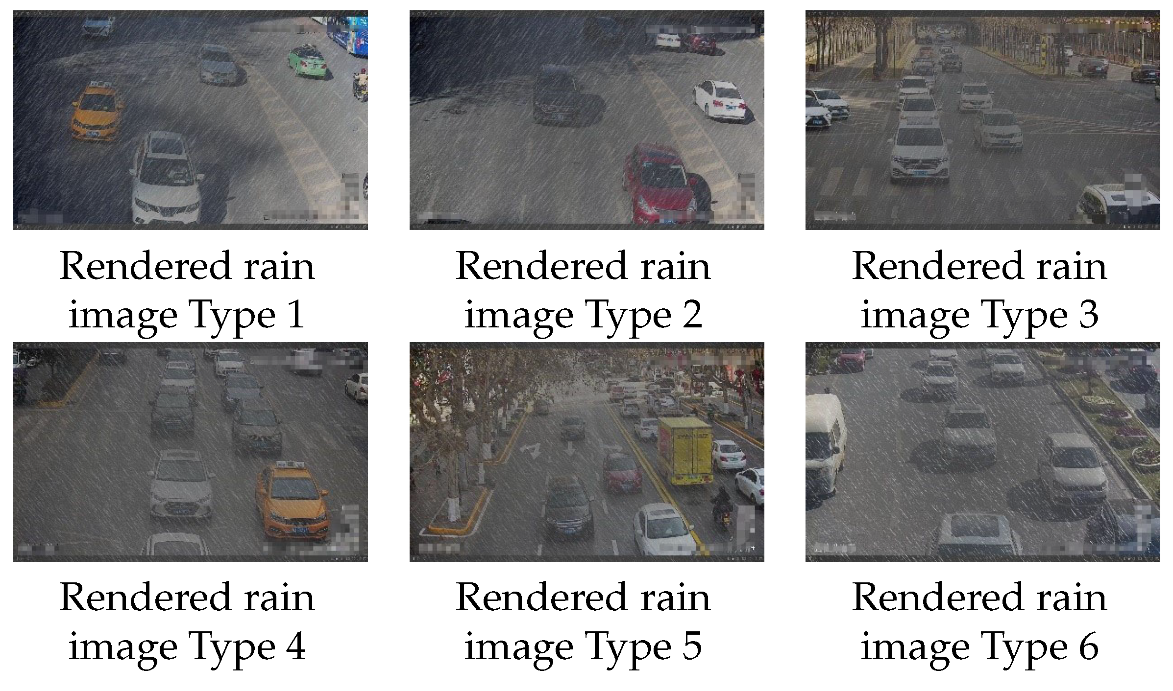
4.2.1. Synthetic Dataset Rain Vehicle Color-24

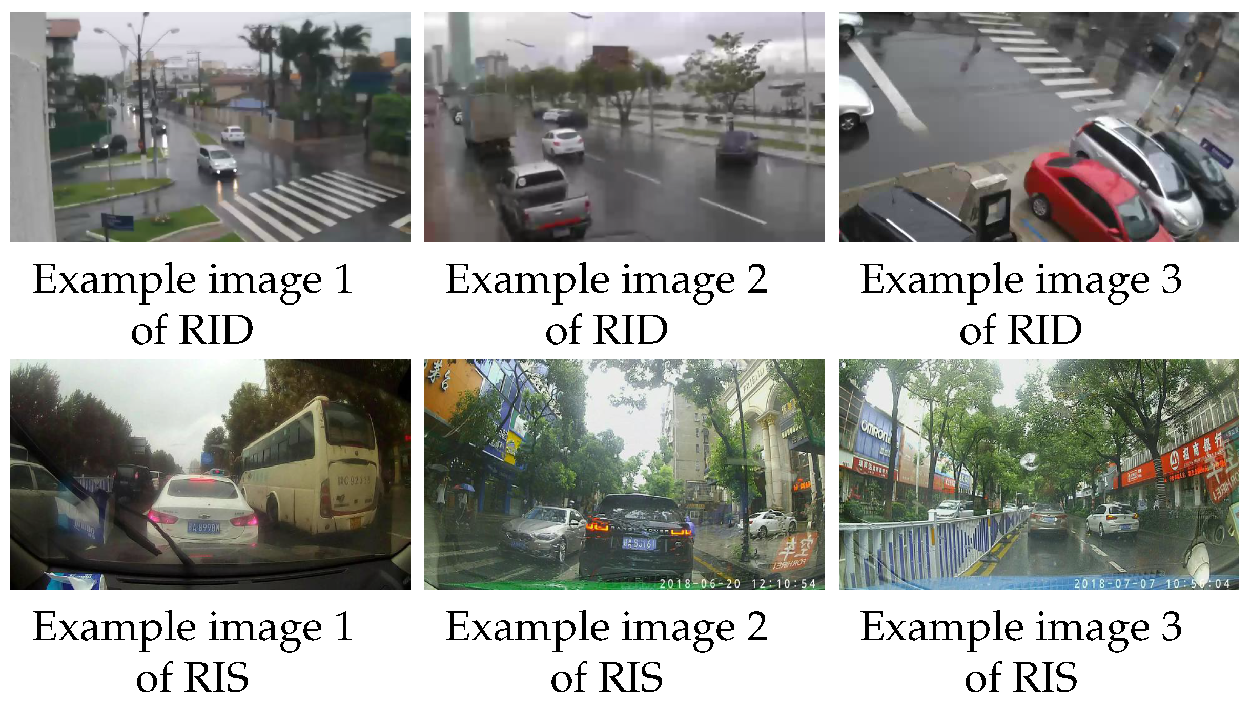
Few datasets are available for vehicle color recognition under rainy weather conditions. All our experiments are conducted on enhanced $RainVehicleColor\text{-}24$ [46], from which some examples are illustrated in Figure 3.

4.2.2. Real Rain Vehicle Datasets: $RID$ and $RIS$

Li et al. collected two real rainy image vehicle datasets, $RID$ and $RIS$[38], for testing object detection. $RID$ is rainy images collected from in-vehicle cameras while driving on rainy days, and $RIS$ is surveillance rainy images collected from network traffic surveillance cameras during rainy weather conditions. The two datasets differ in many aspects: rainfall type, image quality, target size and angle, etc. They represent real-world application scenarios where deraining may be required. $RID$ includes 2495 images, and its rainy image effect is closest to “raindrops” on the camera lens. $RIS$ includes 2048 images, and its rainy image effect is closest to “rain and fog” (many cameras have fog condensation when it rains, and lower resolutions also cause more fog effects) [47]. Due to the highly complex scenes of these two rainy image datasets, it is a challenging dataset, and we choose these two datasets for testing to better illustrate the effectiveness of our proposed algorithm. Examples of these two datasets are given in Figure 4.

4.3. Ablation Study

To determine the optimal design of our proposed framework, we train four combinations on the $RainVehicleColor\text{-}24$ dataset: $RetinaNet$, $JADAR1$, $JADAR2$, and $JADAR$. All these models are trained and tested on $RainVehicleColor\text{-}24$ using different loss functions: $\lambda$ = 0, 0.1, 1.0, and 0.5, respectively. Figure 5 shows that the testing $mAP$ values of the $JADAR1$, $JADAR2$, and $JADAR$ models are 2.92%, −3.99%, and 4.3% higher, respectively, than the $RetinaNet$ model, which clarifies that joint semantic feature extraction is beneficial to improve vehicle color recognition performance under rainy weather conditions. Referring to

Table 1. The mAPs using different values for the loss function coefficient $\lambda$ of the deraining module in $JADAR$ on the $RVC\text{-}24$ test set.

$\mathit{\lambda }$	Model	mAP
0.1	$JADAR1$	70.69%
0.5	$JADAR$	72.07%
1.0	$JADAR2$	63.78%

, when the hyper-parameter $\lambda$ is $0.1$, the rain removal module provides a weak assisting effect on vehicle color recognition under rainy weather conditions. When $\lambda$ is $1.0$, it plays the opposite effect. When $\lambda$ is $0.5$, $JADAR$ performs best; so we choose this value in our method.

4.4. Experiments and Analysis

4.4.1. Results on Synthetic Datasets

In this section, our proposed algorithm, the vehicle color recognition method, the target detection method, the two-stage method combining rain removal with target detection, and the transfer learning method are compared.

To discuss vehicle color recognition performance, $JADAR$ and $SMNN\text{-}MSFF$ [18] are compared. Both are trained on $RainVehicleColor\text{-}24$ training subset and tested on its test subset. The quantitative results are shown in the second column of

Table 2. Comparison of recognition accuracy of 24 colors for different network classifications: SM, SMNN-MSFF; FR, Faster RCNN; Yolo, Yolo V3; RN, RetinaNet.

Category (R, G, B)	SM	FR	Yolo	SSD	RN	JADAR
white (255, 255, 255)	0.60	0.96	0.95	0.95	0.97	0.97
black (0, 0, 0)	0.69	0.69	0.92	0.93	0.93	0.95
orange (237, 145, 33)	0.77	0.90	0.93	0.95	0.97	0.94
silver-gray (128, 138, 135)	0.31	0.81	0.86	0.86	0.86	0.85
grass-green (0, 255, 0)	0.82	0.93	0.95	0.96	0.96	0.96
dark-gray (128, 128, 105)	0.43	0.69	0.63	0.67	0.64	0.73
dark-red (156, 102, 31)	0.48	0.79	0.75	0.88	0.91	0.91
gray (192, 192, 192)	0.31	0.41	0.15	0.31	0.27	0.36
red (255, 0, 0)	0.44	0.56	0.60	0.76	0.77	0.83
cyan (0, 255, 255)	0.62	0.82	0.81	0.87	0.87	0.93
champagne (255, 227, 132)	0.28	0.74	0.58	0.73	0.66	0.69
dark-blue (25, 25, 112)	0.52	0.79	0.77	0.75	0.86	0.81
blue (0, 0, 255)	0.56	0.69	0.55	0.69	0.67	0.69
dark-brown (94, 38, 18)	0.35	0.18	0.40	0.47	0.37	0.50
brown (128, 128, 42)	0.35	0.10	0.22	0.34	0.30	0.21
yellow (255, 255, 0)	0.35	0.83	0.74	0.92	0.86	0.81
lemon-yellow (255, 215, 0)	0.57	0.99	0.73	0.75	0.75	0.94
dark-orange (210, 105, 30)	0.32	0.28	0.44	0.47	0.90	0.53
dark-green (48, 128, 20)	0.59	0.18	0.00	0.34	0.44	0.55
red-orange (255, 97, 0)	0.38	0.07	0.00	0.52	0.00	0.05
earthy-yellow (184, 134, 11)	0.68	0.45	0.00	0.28	0.93	1.00
green (0, 255, 0)	0.18	0.85	0.00	0.97	0.60	0.33
pink (255, 192, 203)	0.84	0.54	0.00	0.52	0.77	0.75
purple (160, 32, 240)	0.22	0.03	0.00	0.06	0.00	1.00
mAP	48.58%	60.65%	49.88%	66.33%	67.77%	72.07%

. These quantitative results confirm that the $mAP$ of our method reaches $72.07\%$, which is $23.49\%$ higher than $SMNN\text{-}MSFF$. The qualitative results are shown in Figure 6. $JADAR$ outperforms $SMNN\text{-}MSFF$ under rainy conditions; for example, there are five vehicles recognized by $JADAR$, while three vehicles are recognized by $SMNN\text{-}MSFF$. A white vehicle is recognized by $JADAR$ with a confidence score of $0.79$, while $SMNN\text{-}MSFF$ recognizes it with a confidence score of $0.62$.

To compare object detection performance, $JADAR$, $RetinaNet$ [24], $Faster$$RCNN$ [19], $SSD$ [20], and $YOLOV3$ [21] are compared qualitatively and evaluated by $mAP$ quantitatively. In our experiments, the loss function and settings (i.e., scale, anchor or default box, backbone network, classifier, etc.) of each compared method remains unchanged from the original work. Furthermore, all methods are trained on the $RainVehicleColor\text{-}24$ dataset and tested on its test set. The qualitative results of $JADAR$, $Faster$$RCNN$, $YOLOV3$, $SSD$, and $RetinaNet$ for vehicle color recognition in rain are shown in Figure 7 and Figure 8. As can be seen from the figures, our proposed $JADAR$ outperforms other models for fine vehicle color recognition. The quantitative results show that the proposed $JADAR$ is $11.42\%$, $22.19\%$, $5.74\%$, and $4.3\%$ better than $Faster$$RCNN$, $YOLOV3$, $SSD$ and $RetinaNet$, respectively, from Table 2.

To compare recognition performances of different joint methods, three state-of-the-art rain removal methods, i.e., $LPNet$ [35], $PReNet$ [48], and $RCDNet$ [49]), are chosen to first derain the images, and then $RetinaNet$ is leveraged to recognize vehicle colors. These methods are denoted $LR$, $PR$, and $RR$. Figure 9 and Figure 10 give qualitative comparisons of our $JADAR$ and three two-stage methods for vehicle color recognition under rainy weather conditions. $JADAR$ performs better than other models. From

Table 3. Comparison of recognition accuracy of 24 colors for different network classifications.

Category (R, G, B)	LR	PR	RR	Da-Faster	ATF	JADAR
white (255, 255, 255)	0.88	0.86	0.95	0.74	0.93	0.97
black (0, 0, 0)	0.75	0.75	0.92	0.61	0.87	0.95
orange (237, 145, 33)	0.91	0.92	0.96	0.73	0.90	0.94
silver-gray (128, 138, 135)	0.71	0.66	0.82	0.63	0.63	0.85
grass-green (0, 255, 0)	0.84	0.88	0.95	0.73	0.92	0.96
dark-gray (128, 128, 105)	0.55	0.44	0.73	0.38	0.65	0.73
dark-red (156, 102, 31)	0.67	0.75	0.87	0.54	0.66	0.91
gray (192, 192, 192)	0.27	0.20	0.37	0.19	0.27	0.36
red (255, 0, 0)	0.74	0.70	0.87	0.46	0.63	0.83
cyan (0, 255, 255)	0.81	0.78	0.92	0.75	0.93	0.93
champagne (255, 227, 132)	0.42	0.43	0.62	0.18	0.67	0.69
dark-blue (25, 25, 112)	0.58	0.30	0.67	0.16	0.89	0.81
blue (0, 0, 255)	0.33	0.48	0.53	0.44	0.92	0.69
dark-brown (94, 38, 18)	0.44	0.32	0.56	0.37	0.75	0.50
brown (128, 128, 42)	0.33	0.25	0.45	0.06	0.00	0.21
yellow (255, 255, 0)	0.79	0.77	0.89	0.39	1.00	0.81
lemon-yellow(255, 215, 0)	0.77	0.78	0.97	0.06	0.00	0.94
dark-orange (210, 105, 30)	0.56	0.18	0.90	1.00	0.00	0.53
dark-green (48, 128, 20)	0.65	0.50	0.95	0.22	0.07	0.55
red-orange (255, 97, 0)	0.00	0.00	0.00	0.39	1.00	0.05
earthy-yellow (184, 134, 11)	0.05	0.67	0.25	0.01	0.40	1.00
green (0, 255, 0)	0.06	0.13	0.00	1.00	1.00	0.33
pink (255, 192, 203)	0.44	0.67	0.67	0.92	0.93	0.75
purple (160, 32,240)	1.00	0.00	1.00	0.00	0.00	1.00
mAP	56.51%	51.70%	70.01%	46.12%	62.93%	72.07%

, our $JADAR$ is $15.56\%$, $20.37\%$, and $2.06\%$ higher than $LR$, $PR$, and $RR$, respectively.

To compare with transfer learning methods, two domain-adaptation methods, $Da$-$faster$ [33] and $ATF$ [50], are compared with $JADAR$. Here, the $VC\text{-}24$ is the source domain, and $RainVehicleColor\text{-}24$ is the target domain; they are leveraged to train the above algorithms. From the $5\text{-}$th and $6\text{-}$th columns of Table 3, our method is 25.95% and 9.14% better than $Da\text{-}faster$ and $ATF$, respectively. The qualitative results in Figure 9 and Figure 10 show that JADAR identifies more vehicles with higher confidence than the other two methods.

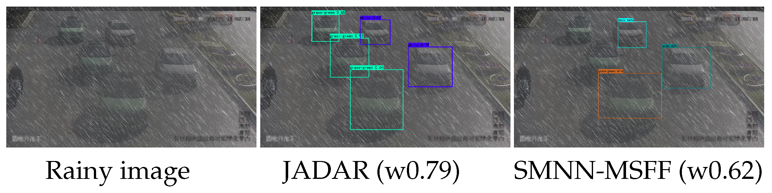
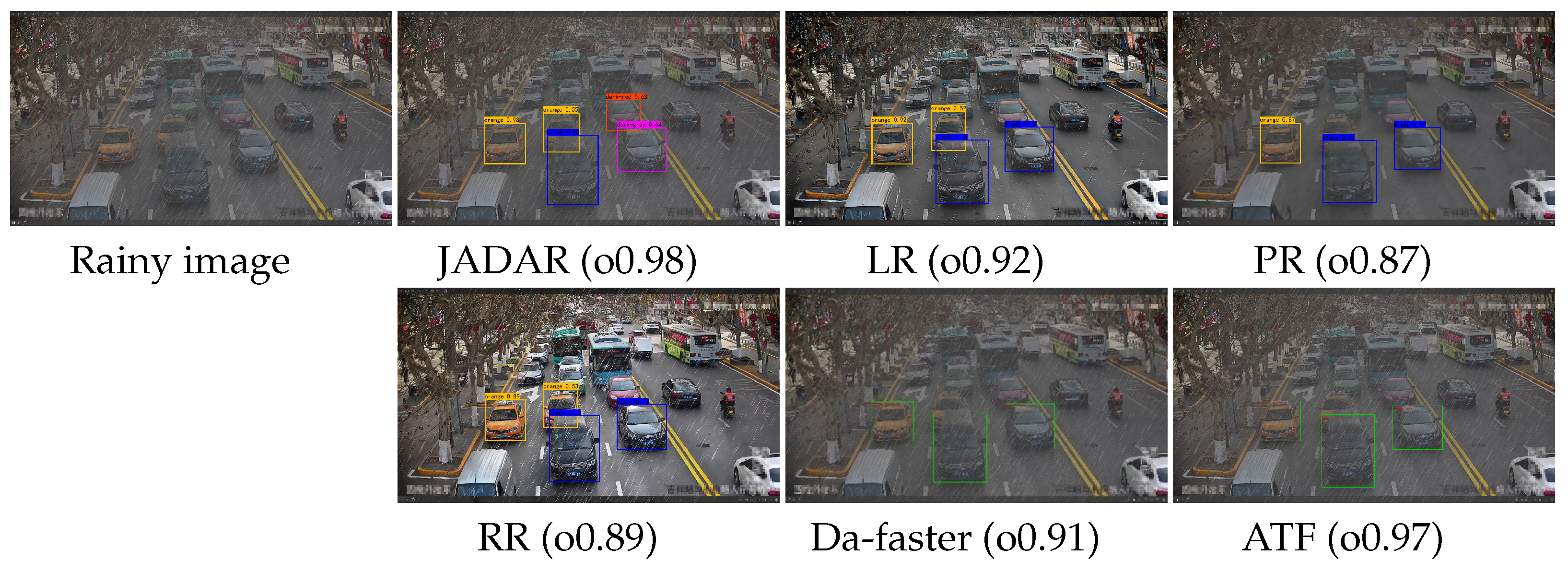
4.4.2. Results on Real Datasets

We train $JADAR$, $RetinaNet$, $Faster$$RCNN$, $SSD$, $YOLOV3$, $LR$, $PR$, $RR$, $Da$-$faster$, and $ATF$ on $Rain$$Vehicle$$Color\text{-}24$ and test them on real rainy image vehicle datasets, $RID$ and $RIS$. The test results are shown in Figure 11, Figure 12, Figure 13 and Figure 14. As can be seen from these figures, the test results of $JADAR$ on the real datasets, $RID$ and $RIS$, are generally better than those of other methods. As can be seen from Figure 11, the $JADAR$ and $SSD$ algorithms can correctly identify the two cars in the picture; $YoloV3$ can also identify the two cars in the picture, but the black color is mistakenly identified as silver-gray; while the other three algorithms can hardly identify any vehicles in the picture. Referring to Figure 12, because the recognition effects of $FasterRCNN$ and $SSD$ are better than others’, we find a limitation of $JADAR$ in recognizing small targets. Referring to Figure 13, all algorithms can identify the color of the vehicle in the image but with different confidence values; specifically, $ATF$ has the highest confidence value for blue vehicle, with $0.98$. However, Figure 14 shows that only $JADAR$ and $ATF$ can identify a certain white vehicle.

4.5. Inference Time

In order to compare the test time of all methods, all network models are tested on a testing subset with an input of $1920\times 1080$ images. The test times are shown in

Table 4. Comparison of different network recognition speeds (GPU).

Algorithm	RN	LR	PR	RR	Da-Faster	ATF	JADAR
Speed (s)	1.7	23.5	2.8	6.1	2.5	2.6	1.7

. JADAR takes 1.7 s per image on a single Tesla $P40$ GPU, which is the same as for $RetinaNet$, but JADAR is 21.8, 1.1, 4.4, 0.8, and 0.9 seconds faster than $LR$, $PR$ and $RR$, $Da\text{-}faster$, and $ATF$, respectively. Therefore, although $JADAR$ has one more decoder module than $RetinaNet$, it still maintains its original high detection speed.

5. Conclusions

In this paper, we study vehicle color recognition under rainy conditions and propose a joint semantics learning method $JADAR$, which is designed by embedding $UNet\text{-}3$ into $RetinaNet$. The $UNet$ module achieves rainy image removal and restores the clean background image. The recovered background image and the rainy image are input together into the $class+bbox$ sub-module of $RetinaNet$ network to accurately extract the joint semantic of the vehicle color features maps. $JADAR$ outperforms other methods under rainy as well as normal conditions for fine vehicle color recognition. Extensive experimental results show that the $mAP$ of the proposed method reaches $72.07\%$ in identifying 24 colors under rainy conditions. Because our algorithm is trained on synthetic datasets, its generalization is not guaranteed. In the future, semi-supervised or few-shot learning is planned to further improve the generalization and realizability of the algorithm. As a further research topic, one can consider fusing overlap functions and fuzzy (rough) sets (see [51,52,53,54,55]) to develop the method of this paper.

References

1. Tang, J.; Zeng, J. Spatiotemporal gated graph attention network for urban traffic flow prediction based on license plate recognition data. Comput.-Aided Civ. Infrastruct. Eng. 2022, 37, 3–23. [Google Scholar] [CrossRef]
2. Rajavel, R.; Ravichandran, S.K.; Harimoorthy, K.; Nagappan, P.; Gobichettipalayam, K.R. IoT-based smart healthcare video surveillance system using edge computing. J. Ambient. Intell. Humaniz. Comput. 2022, 13, 3195–3207. [Google Scholar] [CrossRef]
3. Wang, Z.; Zhan, J.; Duan, C.; Guan, X.; Lu, P. A review of vehicle detection techniques for intelligent vehicles. IEEE Trans. Neural Netw. Learn. Syst. 2022, 23, 1–21. [Google Scholar] [CrossRef]
4. Wang, J.; Gao, J.; Zhao, S.; Zhu, R.; Jiang, Z. From Model to Algorithms: Distributed Magnetic Sensor System for Vehicle Tracking. IEEE Trans. Ind. Inform. 2022, 33, 1. [Google Scholar] [CrossRef]
5. Lee, S.; Park, S.H. Concept drift modeling for robust autonomous vehicle control systems in time-varying traffic environments. Expert Syst. Appl. 2022, 190, 116–206. [Google Scholar] [CrossRef]
6. Khan, M.A.; Sayed, H.E.; Malik, S.; Zia, T.; Khan, J. Level-5 Autonomous Driving—Are We There Yet? A Review of Research Literature. ACM Comput. Surv. 2022, 55, 1–38. [Google Scholar] [CrossRef]
7. Custers, B. AI in Criminal Law: An Overview of AI Applications in Substantive and Procedural Criminal Law. In Law and Artificial Intelligence; Asser Press: The Hague, The Netherlands, 2022; pp. 205–223. [Google Scholar]
8. Chen, P.; Bai, X.; Liu, W. Vehicle color recognition on urban road by feature context. IEEE Trans. Intell. Transp. Syst. 2014, 15, 2340–2346. [Google Scholar] [CrossRef]
9. Jeong, Y.; Park, K.H.; Park, D. Homogeneity patch search method for voting-based efficient vehicle color classification using front-of-vehicle image. Multimed. Tools Appl. 2019, 78, 28633–28648. [Google Scholar] [CrossRef]
10. Tilakaratna, D.S.; Watchareeruetai, U.; Siddhichai, S.; Natcharapinchai, N. Image analysis algorithms for vehicle color recognition. In Proceedings of the 2017 International Electrical Engineering Congress, Pattaya, Thailand, 8–10 March 2017; pp. 1–4. [Google Scholar]
11. Dule, E.; Gokmen, M.; Beratoglu, M.S. A convenient feature vector construction for vehicle color recognition. In Proceedings of the 11th WSEAS International Conference on Nural Networks and 11th WSEAS International Conference on Evolutionary Computing and 11th WSEAS International Conference on Fuzzy Systems, Iasi Romania, 13–15 June 2010; pp. 250–255. [Google Scholar]
12. Hu, C.; Bai, X.; Qi, L.; Chen, P.; Xue, G. Vehicle color recognition with spatial pyramid deep learning. IEEE Trans. Intell. Transp. Syst. 2015, 16, 2925–2934. [Google Scholar] [CrossRef]
13. Rachmadi, R.F.; Purnama, I.K. Vehicle color recognition using convolutional neural network. In Proceedings of the IEEE International Conference on Computer Vision and Pattern Recognition, Boston, MA, USA, 7–10 June 2015. [Google Scholar]
14. Zhuo, L.; Zhang, Q.; Li, J.; Zhang, J.; Li, X. High-accuracy vehicle color recognition using hierarchical fine-tuning strategy for urban surveillance videos. J. Electron. Imaging 2018, 27, 1–9. [Google Scholar] [CrossRef]
15. Zhang, Q.; Zhuo, L.; Li, J.; Zhang, J.; Zhang, H. Vehicle color recognition using Multiple-Layer Feature Representations of lightweight convolutional neural network. Signal Process. 2018, 147, 146–153. [Google Scholar] [CrossRef]
16. Fu, H.; Ma, H.; Wang, G.; Zhang, X.; Zhang, Y. Mcff-cnn: Multiscale comprehensive feature fusion convolutional neural network for vehicle color recognition based on residual learning. Neurocomputing 2020, 395, 178–187. [Google Scholar] [CrossRef]
17. Nafzi, M.; Brauckmann, M.; Glasmachers, T. Vehicle shape and color classification using convolutional neural network. In Proceedings of the IEEE International Conference on Computer Vision and Pattern Recognition, Long Beach, CA, USA, 16–21 June 2019. [Google Scholar]
18. Hu, M.; Bai, L.; Li, Y.; Zhao, S.R.; Chen, E.H. Vehicle Color Recognition Based on Smooth Modulation Neural Network with Multi-Scale Feature Fusion. arXiv 2021, arXiv:2107.09944. [Google Scholar]
19. Ren, S.; He, K.; Girshick, R.; Sun, J. Faster r-cnn: Towards real-time object detection with region proposal networks. IEEE Trans. Pattern Anal. Mach. Intell. 2017, 39, 1137–1149. [Google Scholar] [CrossRef]
20. Liu, W.; Anguelov, D.; Erhan, D.; Szegedy, C.; Reed, S. Ssd: Single shot multi-box detector. In Proceedings of the European Conference on Computer Vision, Amsterdam, The Netherlands, 8–16 October 2016; pp. 21–37. [Google Scholar]
21. Redmon, J.; Divvala, S.; Girshick, R.; Farhadi, A. You only look once: Unified, real-time object detection. In Proceedings of the 2016 IEEE Conference on Computer Vision and Pattern Recognition, Las Vegas, NV, USA, 27–30 June 2016; pp. 779–788. [Google Scholar]
22. Bochkovskiy, A.; Wang, C.Y.; Liao, H.Y. Yolov4: Optimal speed and accuracy of object detection. In Proceedings of the 2020 IEEE Conference on Computer Vision and Pattern Recognition, Seattle, WA, USA, 13–19 June 2020. [Google Scholar]
23. Tan, M.; Pang, R.; Le, Q.V. Efficientdet: Scalable and efficient object detection. In Proceedings of the 2020 IEEE Conference on Computer Vision and Pattern Recognition, Seattle, WA, USA, 13–19 June 2020; pp. 10781–10790. [Google Scholar]
24. Lin, T.Y.; Goyal, P.; Girshick, R.; He, K.; Dollár, P. Focal loss for dense object detection. In Proceedings of the 2017 IEEE Conference on Computer Vision and Pattern Recognition, Honolulu, HI, USA, 21–26 July 2017; pp. 2980–2988. [Google Scholar]
25. Xu, M.; Wang, H.; Ni, B.; Tian, Q.; Zhang, W. Cross-domain detection via graph-induced prototype alignment. In Proceedings of the IEEE/CVF Conference on Computer Vision and Pattern Recognition, Seattle, WA, USA, 13–19 June 2020; pp. 12355–12364. [Google Scholar]
26. Zhang, Y.; Wang, Z.; Mao, Y. Rpn prototype alignment for domain adaptive object detector. In Proceedings of the IEEE/CVF Conference on Computer Vision and Pattern Recognition, Nashville, TN, USA, 20–25 June 2021; pp. 12425–12434. [Google Scholar]
27. Kim, T.; Jeong, M.; Kim, S.; Choi, S.; Kim, C. Diversify and match: A domain adaptive representation learning paradigm for object detection. In Proceedings of the IEEE/CVF Conference on Computer Vision and Pattern Recognition, Long Beach, CA, USA, 15–20 June 2019; pp. 12456–12465. [Google Scholar]
28. Dong, H.; Pan, J.; Xiang, L.; Hu, Z.; Zhang, X.; Wang, F.; Yang, M.H. Multi-scale boosted dehazing network with dense feature fusion. In Proceedings of the IEEE/CVF Conference on Computer Vision and Pattern Recognition, Seattle, WA, USA, 13–19 June 2020; pp. 2157–2167. [Google Scholar]
29. Xu, C.D.; Zhao, X.R.; Jin, X.; Wei, X.S. Exploring categorical regularization for domain adaptive object detection. In Proceedings of the IEEE/CVF Conference on Computer Vision and Pattern Recognition, Seattle, WA, USA, 13–19 June 2020; pp. 11724–11733. [Google Scholar]
30. Vs, V.; Gupta, V.; Oza, P.; Sindagi, V.A.; Patel, V.M. Mega-cda: Memory guided attention for category-aware unsupervised domain adaptive object detection. In Proceedings of the IEEE/CVF Conference on Computer Vision and Pattern Recognition, Nashville, TN, USA, 20–25 June 2021; pp. 4516–4526. [Google Scholar]
31. Sindagi, V.A.; Oza, P.; Yasarla, R.; Patel, V.M. Prior-based domain adaptive object detection for hazy and rainy conditions. In Proceedings of the European Conference on Computer Vision, Glasgow, UK, 23–28 August 2020; Springer: Berlin/Heidelberg, Germany, 2020; pp. 763–780. [Google Scholar]
32. Wang, T.; Zhang, X.; Yuan, L.; Feng, J. Few-shot adaptive faster r-cnn. In Proceedings of the IEEE/CVF Conference on Computer Vision and Pattern Recognition, Long Beach, CA, USA, 15–20 June 2019; pp. 7173–7182. [Google Scholar]
33. Chen, Y.; Li, W.; Sakaridis, C.; Dai, D.; Van, G.L. Domain adaptive faster rcnn for object detection in the wild. In Proceedings of the European Conference on Computer Vision, Munich, Germany, 8–14 September 2018; pp. 3339–3348. [Google Scholar]
34. Liu, W.; Ren, G.; Yu, R.; Guo, S.; Zhu, J. Image-adaptive yolo for object detection in adverse weather conditions. In Proceedings of the AAAI Conference on Artificial Intelligence, Arlington, VA, USA, 17–19 November 2022; pp. 1792–1800. [Google Scholar]
35. Fu, X.; Liang, B.; Huang, Y.; Ding, X.; Paisley, J. Lightweight pyramid networks for image deraining. IEEE Trans. Neural Netw. Learn. Syst. 2019, 31, 1794–1807. [Google Scholar] [CrossRef]
36. Fan, Z.; Wu, H.; Fu, X.; Hunag, Y.; Ding, X. Residual-guide feature fusion network for single image deraining. arXiv 2018, arXiv:1804.07493. [Google Scholar]
37. Jiang, K.; Wang, Z.; Yi, P.; Chen, C.; Huang, B. Multi-scale progressive fusion network for single image deraining. In Proceedings of the IEEE/CVF Conference on Computer Vision and Pattern Recognition, Seattle, WA, USA, 13–19 June 2020; pp. 8346–8355. [Google Scholar]
38. Li, S.Y.; Araujo, I.B.; Ren, W.Q.; Wang, Z.Y.; Tokuda, E.K. Single image deraining: A comprehensive benchmark analysis. In Proceedings of the 2019 IEEE/CVF Conference on Computer Vision and Pattern Recognition, Long Beach, CA, USA, 15–20 June 2019; pp. 3833–3842. [Google Scholar]
39. Tremblay, M.; Halder, S.S.; De Charette, R.; Lalonde, J.F. Rain rendering for evaluating and improving robustness to bad weather. Int. J. Comput. Vis. 2021, 129, 341–360. [Google Scholar] [CrossRef]
40. Zhang, H.; Sindagi, V.; Patel, V.M. Image de-raining using a conditional generative adversarial network. IEEE Trans. Circuits Syst. Video Technol. 2020, 30, 3943–3956. [Google Scholar] [CrossRef]
41. Huang, S.C.; Le, T.H.; Jaw, D.W. DSNet: Joint semantic learning for object detection in inclement weather conditions. IEEE Trans. Pattern Anal. Mach. Intell. 2020, 43, 2623–2633. [Google Scholar] [CrossRef]
42. Hu, M.; Yang, J.; Lin, N.; Liu, Y.; Fan, J. Lightweight single image deraining algorithm incorporating visual saliency. IET Image Process. 2022, 16, 3190–3200. [Google Scholar] [CrossRef]
43. Ronneberger, O.; Fischer, P.; Brox, T. U-net: Convolutional networks for biomedical image segmentation. In Proceedings of the International Conference on Medical Image Computing and Computer-Assisted Intervention, Munich, Germany, 5–9 October 2015; Springer: Cham, Switzerland, 2015; pp. 234–241. [Google Scholar]
44. Kingma, D.P.; Ba, J. Adam: A method for stochastic optimization. arXiv 2014, arXiv:1412.6980. [Google Scholar]
45. Jose, H.; Vadivukarasi, T.; Devakumar, J. Extraction of protein interaction data: A comparative analysis of methods in use. EURASIP J. Bioinform. Syst. Biol. 2007, 43, 53096. [Google Scholar] [CrossRef] [PubMed]
46. Hu, M.; Wang, C.; Yang, J.; Wu, Y.; Fan, J.; Jing, B. Rain Rendering and Construction of Rain Vehicle Color-24 Dataset. Mathematics 2022, 10, 3210. [Google Scholar] [CrossRef]
47. Hu, M.; Wu, Y.; Song, Y.; Yang, J.B.; Zhang, R.F. The integrated evaluation and review of single image rain removal based datasets and deep methods. J. Image Graph. 2022, 27, 1359–1391. [Google Scholar]
48. Ren, D.; Zuo, W.; Hu, Q.; Zhu, P.; Meng, D.Y. Progressive image deraining networks: A better and simpler baseline. In Proceedings of the 2019 IEEE/CVF Conference on Computer Vision and Pattern Recognition, Long Beach, CA, USA, 15–20 June 2019; pp. 3937–3946. [Google Scholar]
49. Wang, H.; Xie, Q.; Zhao, Q.; Meng, D.Y. A model-driven deep neural network for single image rain removal. In Proceedings of the 2020 IEEE/CVF Conference on Computer Vision and Pattern Recognition, Seattle, WA, USA, 14–19 June 2020; pp. 3100–3109. [Google Scholar]
50. He, Z.; Zhang, L. Domain adaptive object detection via asymmetric tri-way faster-rcnn. In Proceedings of the European Conference on Computer Vision, Glasgow, UK, 23–28 August 2020; Springer: Cham, Switzerland, 2020; pp. 309–324. [Google Scholar]
51. Liang, R.; Zhang, X. Interval-valued pseudo overlap functions and application. Axioms 2022, 11, 216. [Google Scholar] [CrossRef]
52. Wang, J.; Zhang, X. A novel multi-criteria decision-making method based on rough sets and fuzzy measures. Axioms 2022, 11, 275. [Google Scholar] [CrossRef]
53. Zhang, X.; Wang, J.; Zhan, J.; Dai, J. Fuzzy measures and Choquet integrals based on fuzzy covering rough sets. IEEE Trans. Fuzzy Syst. 2021, 30, 2360–2374. [Google Scholar] [CrossRef]
54. Sheng, N.; Zhang, X. Regular partial residuated lattices and their filters. Mathematics 2022, 10, 2429. [Google Scholar] [CrossRef]
55. Wang, J.; Zhang, X.; Hu, Q. Three-way fuzzy sets and their applications (II). Axioms 2022. under review of the second version. [Google Scholar]
Figure 1. Framework overview for our J A D A R ; detailed explanations are in the text.
Mathematics 10 03512 g001
Figure 2. Architecture and weights of the proposed network in detail.
Mathematics 10 03512 g002
Figure 3. Examples from R a i n V e h i c l e C o l o r - 24 .
Mathematics 10 03512 g003
Figure 4. Examples of RID and RIS images [38].
Mathematics 10 03512 g004
Figure 5. A P s of different models on the Rain Vehicle Color-24 test set. The x-axis represents the average precision, and the y - axis represents the color categories (24 categories in total).
Mathematics 10 03512 g005
Figure 6. Test results of J A D A R and S M N N - M S F F on the Rain Vehicle Color-24 test set. Each subtitle gives object detection method with the corresponding confidence value in parentheses.
Mathematics 10 03512 g006
Figure 7. Example 1 of test results of JADAR and object detection methods on the Rain Vehicle Color-24 test set.
Mathematics 10 03512 g007
Figure 8. Example 2 of test results of JADAR and object detection methods and domain adaptation methods on the Rain Vehicle Color-24 test set.
Mathematics 10 03512 g008
Figure 9. Example 1 of test results of JADAR and two-stage methods on the Rain Vehicle Color-24 test set.
Mathematics 10 03512 g009
Figure 10. Example 2 of test results of JADAR and two-stage methods and domain-adaptation methods on the Rain Vehicle Color-24 test set.
Mathematics 10 03512 g010
Figure 11. Test results of JADAR and color recognition and object detection methods on the RID.
Mathematics 10 03512 g011
Figure 12. Test results of JADAR and color recognition and object detection methods on the RIS.
Mathematics 10 03512 g012
Figure 13. Test results of JADAR and two-stage and domain-adaptation methods on the RID.
Mathematics 10 03512 g013
Figure 14. Test results of J A D A R and two-stage and domain-adaptation methods on the R I S .
Mathematics 10 03512 g014