Network Thermodynamics-Based Scalable Compartmental Model for Multi-Strain Epidemics

Abstract

SARS-CoV-2 continues to upend human life by posing novel threats related to disease spread and mutations. Current models for the disease burden of SARS-CoV-2 consider the aggregate nature of the virus without differentiating between the potency of its multiple strains. Hence, there is a need to create a fundamental modeling framework for multi-strain viruses that considers the competing viral pathogenic pathways. Alongside the consideration that other viral pathogens may coexist, there is also a need for a generalizable modeling framework to account for multiple epidemics (i.e., multi-demics) scenarios, such as influenza and COVID-19 occurring simultaneously. We present a fundamental network thermodynamics approach for assessing, determining, and predicting viral outbreak severity, which extends well-known standard epidemiological models. In particular, we use historical data from New York City’s 2011–2019 influenza seasons and SARS-CoV-2 spread to identify the model parameters. In our model-based analysis, we employ a standard susceptible–infected–recovered (SIR) model with pertinent generalizations to account for multi-strain and multi-demics scenarios. We show that the reaction affinities underpinning the formation processes of our model can be used to categorize the severity of infectious or deceased populations. The spontaneity of occurrence captured by the change in Gibbs free energy of reaction ($∆G$) in the system suggests the stability of forward occurring population transfers. The magnitude of $∆G$ is used to examine past influenza outbreaks and infer epidemiological factors, such as mortality and case burden. This method can be extrapolated for wide-ranging utility in computational epidemiology. The risk of overlapping multi-demics seasons between influenza and SARS-CoV-2 will persist as a significant threat in forthcoming years. Further, the possibility of mutating strains requires novel ways of analyzing the network of competing infection pathways. The approach outlined in this study allows for the identification of new stable strains and the potential increase in disease burden from a complex systems perspective, thereby allowing for a potential response to the significant question: are the effects of a multi-demic greater than the sum of its individual viral epidemics?

1. Introduction

The emergence of severe acute respiratory syndrome coronavirus 2 (SARS-CoV-2) has renewed the urgency of new epidemiological studies. SARS-CoV-2 has infected over 200 million people worldwide leading to over 4 million fatalities through August 2021. Estimates suggest that SARS-CoV-2 case-fatality rates vary between 1.4% (India) and 3.5% (Peru) and as high as 8.8% (Mexico) [1]. Early estimates from China suggest that at least 18.4% of those infected over the age of 80 will be hospitalized. With high transmissibility and prevalence, the emerging SARS-CoV-2 variants—including Alpha, Beta, Gamma, Epsilon, Delta, and so on—have piqued interest and urgency in classifying emergent viral dynamics. Hence, model-based analyses will play an important role in guiding our fight against the current SARS-CoV-2 outbreak [2].

In compartmental model-based epidemiology, metrics pertaining to infection, exposition, hospitalization, death, etc., are characterized through interaction within the population. A vast array of compartmental models have been proposed to analyze infectious diseases. Compartmental modeling methods are so ubiquitous that their archetypes can be marginally modified to produce models capable of capturing the complex dynamics of many different infectious outbreaks [3,4]. Early in the progression of SARS-CoV-2, SIR models were employed to make estimates about severity [5,6]. Large meta-population network transmission models provided inter-neighborhood information about the SARS-CoV-2 outbreak of Spring 2020 in New York City [7] and helped inform public health decisions. In computational epidemiology, widely used SIR models abstract simple directed networks of representative compartments that illustrate the flow of infected individuals between the compartments. For the purposes of modeling the SARS-CoV-2 pandemic, it is increasingly apparent that the complexity of compartmental models must be increased such that models are at least “complex enough” [8]. Researchers have designed several specifically adapted compartmental models to represent the SARS-CoV-2 pandemic [9,10,11,12].

Here, we propose that these increasingly complex compartmental models can be expressed as directed graphs that are well suited for network thermodynamic (NT) analyses [13] as a means to deduce the severity of an outbreak, and stability of emergent strains. The NT modeling paradigm allows for parameter lumping, which can maintain the model complexity needed for complex biological processes while reducing dimensionality and maintaining parameter explainability. NT analytical tools allow for stability assumptions in emergent strains similar to the theory of chemostat [14], with small additional computational expense and wide adaptability to existing compartmental models. In this context, thermodynamic methods become relevant; such methods have much utility in mass-action-based dynamical systems [15,16]—a class of problems closely related to systems defined by compartmental epidemiology-based equations. Our model presents a new form of the classic compartmental model which is generally scalable and can capture the dynamics of emerging viral mutations. In 2015, Browne proposed a model which included emergent strains within-host in the case of incubating human immunodeficiency virus (HIV) [17]. Eletreby et al. highlighted the importance of including evolutionary effects in network approaches to epidemiology by characterizing a threshold by which strains may emerge [18]. Fudolig and Howard devised multi-strain models for influenza in which vaccination gives rise to immunity and mutations [19]. The novelty contained herein lies in the scalability and ability to capture emergent strains within-population. The scalability is such that this modeling paradigm can be easily adapted to SIR-type models of any size. Further, when the NT-based model is trained on concurrent infection data, compartments can be easily added or subtracted to reflect physical observations and further infer the danger of emergent strains.

As model-based epidemiological approaches rely on more complex compartmental networks, the corresponding thermodynamic analysis of affinities between populations provides insight pertaining to the competing nature and stability of the vast network pathways. Previous work toward the theory of chemostat [14] discusses the stability of emergent strains through the arduous composition of Lyapunov functions. De Leenheer and Pilyugin worked out a multistrain model by which Lyapunov stability functions govern the dominant strains [20]. The proposed network thermodynamic approach brings to bear novel tools in the domain of computational epidemiology. Our framework enables the modeling of phase transitions in viral pathways, and, by extension, provides a lens through which threats to public health espoused by twindemics and novel strains can be further classified as a thermodynamic phenomenon.

In the words of Mikulecky [13], “Network thermodynamics is a marriage of classical and non-equilibrium thermodynamics along with network theory and kinetics to provide a practical framework for handling these systems”. This approach, built on the framework of Rosen’s ‘relational theory’ [21], is particularly apt for studying nonlinear dynamical systems which are out of thermodynamic equilibrium by focusing simultaneously on different scales of a system: (a) the larger overall topological structure of the system; and (b) the smaller internal functionality of each component which is captured by their relational aspects and described by the energetic exchanges described by the corresponding models, wherein applying the NT approach in the context of compartmental epidemiology, the stability of emergent strains is abstracted by the energetic exchanges overlayed on the relations in the infection network. The NT approach has found ubiquitous meaning ranging from electrical, biological to chemical networks, but are yet to be implemented in epidemiological investigations. The stability and spontaneity of viral pathways can be cast into a network thermodynamic framework on existing compartmental models. Therefore, the overarching goal of this study is to expand the arsenal of tools in interpreting epidemiological models.

2. Materials and Methods

In this model-based analysis, we employ a fundamental susceptible–infected–removed (SIR) model with modifications for twindemic and emerging strain epidemics. The modeling paradigm is such that the flow between susceptible, infected, recovered and deceased populations is discussed as an exchange along a directed graph, and rate constants capture physical properties, such as infectiousness. Rate constants describing the historical data of Manhattan’s influenza and SARS-CoV-2 epidemics are computed and used to calculate network thermodynamic quantities, which correlate with the stability and activity of viral spread. We first model the individual spread dynamics of both the ongoing SARS-CoV-2 pandemic, and several past flu seasons. Using historical data [1,22] for susceptible population, confirmed infections, and influenza/SARS-CoV-2 deaths, a SIR-type compartmental disease spread model fit is performed. SIR models have thoroughly studied the efficacy in forecasting viral influenza spread [23,24,25], and for informing outbreak control strategies in respiratory disease epidemics [26,27,28]. From the compartmental model, rate constants governing infection and death rates are obtained. These transition rates and fitted models allow the framework to perform a network thermodynamic analysis of the individual spread of a single viral pathogen. By computing the change in Gibbs free energy ($∆G$) describing the thermodynamic spontaneity of the actions between compartments, we suggest a novel technique in analyzing the stability of emergent pathways in viral models, and a predictive tool for model-based epidemiology.

SARS-CoV-2 and influenza data are fit using the method of least squares. The governing equations are solved using a six-stage, fifth-order Runge–Kutta method. These calculations are performed using the MATLAB lsqcurvefit and ode45 functions, respectively.

Table 1. Rate values obtained for corresponding influenza seasons, and the first 100 days since first infection in Manhattan, NY.

Data	($\mathit{\beta },\mathit{\delta }$)	Avg. Standard Score
		Susceptible	Infected	Deceased
10–11 Flu	(1.12668, 1.04069)	1.1300	−0.1352	159.2231
11–12 Flu	(1.01358, 0.98706)	0.6862	2.5187	10.8314
12–13 Flu	(1.14799, 1.04573)	1.3165	−0.0746	9.8953
13–14 Flu	(1.06940, 0.98776)	0.9962	−0.0931	13.3992
14–15 Flu	(1.10619, 0.99636)	1.2201	−0.0875	215.7060
15–16 Flu	(1.15666, 1.06116)	0.8254	−0.1168	379.5621
16–17 Flu	(1.03672, 1.03568)	0.7227	−0.6256	22.4527
COVID-19	(2.84772, 2.76299)	0.6194	−1.9256	31.2687

displays values obtained from the select fits, along with the average standard score by compartment.

2.1. Models

Three models are employed for the purposes of this study. In order to extract infection and death rates, data are fit to a simple SIR-type compartmental spread model (Figure 1a); we say SIR-type because recovered individuals are not captured in their own bin and corresponding assumptions are made to infer the reversibility of the underpinning reactions. Here, S is the susceptible bin, I is the infected bin, and D is the deceased bin. Rather than a traditional removed bin, a deceased bin is used in our data fits to best capture the burden of infectious disease. Furthermore, recovered counts can be easily extrapolated from known infections and deaths. The Centers for Disease Control and Prevention (CDC) defines disease burden by infections and mortality per capita. $\beta$ and $\delta$ correspond to rates entering the infectious and deceased bins. Next, two modified SIR-type models are proposed.

The first twindemic model (Figure 1b) allows the dynamical consequences of two distinct, concurrent epidemics to be explored. Subscripts $c\mathrm{and}f$ denote SARS-CoV-2- and influenza-type rates and bins, respectively. Here R represents the recovered bin, and an existing R binallows the dynamics of both viral pathways to interact. Hence, there exists a connection from $R_c$ to $I_f$ and $R_f$ to $I_c$ showing that one can recover from influenza just to be infected by SARS-CoV-2, and vice versa. Additionally, $\gamma$ is chosen to represent the recovery rate for the corresponding infection. Because data fits are not performed for recovered individuals, we estimate ${\gamma }_i=1-{\delta }_i$ such that if an individual has not perished from SARS-CoV-2 in a certain time, they will recover. This modeling paradigm will allow the individually obtained rate constants to be used on a multi-pathway compartmental model and open our analysis to examining the strife of concurrent flu and SARS-CoV-2 spread.

Second, a model based on emergent strains (Figure 1c) is studied. Here, $\alpha$ represents a mutability parameter—controlling the likelihood of emergent strains mutating. This model is presented as a general structure upon which multi-strain viral outbreaks can be studied based on mutability parameters. Where twindemic covers the spread of concurrent and distinct viruses, the multi-strain model allows the study of viral pathogens which are closely related by mutations of one another, for example, different sub-types of influenza or SARS-CoV-2 and its variants, such as Alpha, Beta, Gamma, Epsilon, or Delta. Figure 1d shows the pathways between the susceptible and deceased nodes in the multi-strain model. These pathways are the subjects by which the following analyses will determine stable and emergent strain variations.

The governing equations for each model are shown below. The simple SIR-type model is used to extract parameters based on historical data. Note that bin concentration data are normalized by the estimated population of NYC.

$$\begin{array}{cc}\hfill \frac{dS}{dt}& =-\beta SI\hfill \end{array}$$

(1)

$$\begin{array}{cc}\hfill \frac{dI}{dt}& =\beta SI-\delta I\hfill \end{array}$$

(2)

$$\begin{array}{cc}\hfill \frac{dD}{dt}& =\delta I\hfill \end{array}$$

(3)

The twindemic model is used to make predictions about concurrently propagating epidemics.

$$\begin{array}{cc}\hfill \frac{dS}{dt}& =-S({\beta }_f{I}_f+{\beta }_c{I}_c)\hfill \end{array}$$

(4)

$$\begin{array}{cc}\hfill \frac{dD}{dt}& ={\delta }_f{I}_f+{\delta }_c{I}_c\hfill \end{array}$$

(5)

$$\begin{array}{cc}\hfill \frac{d{I}_f}{dt}& ={\beta }_{f}S{I}_f-{\delta }_f{I}_f+{\beta }_{f}S{R}_c\hfill \end{array}$$

(6)

$$\begin{array}{cc}\hfill \frac{d{R}_f}{dt}& ={\gamma }_f{I}_f-{\beta }_c{R}_{f}S\hfill \end{array}$$

(7)

$$\begin{array}{cc}\hfill \frac{d{I}_c}{dt}& ={\beta }_{c}S{I}_c-{\delta }_c{I}_c+{\beta }_{c}S{R}_f\hfill \end{array}$$

(8)

$$\begin{array}{cc}\hfill \frac{d{R}_c}{dt}& ={\gamma }_c{I}_c-{\beta }_f{R}_{c}S\hfill \end{array}$$

(9)

Presented in Figure 1c is the simplest possible multi-strain (emergent strain) model containing only one mutation. This model could easily be extrapolated to include any number of distinct viruses, with any amount of possible mutations. For purposes of generality, we will let subscript $i=[1,2\cdots ,n]$ denote n-many viral mutations (e.g., $i=[A,B]$ for Type A and Type B influenza). Thus, the governing equations appear as follows:

$$\begin{array}{cc}\hfill \frac{dS}{dt}& =-S\sum _{i=1}^n{\beta }_i{I}_i\hfill \end{array}$$

(10)

$$\begin{array}{cc}\hfill \frac{d{I}_i}{dt}& ={\beta }_{i}S{I}_i-{\delta }_i{I}_i-I_i\sum _{j=1}^{n-1}\left({\alpha }_j\right)+{\alpha }_i\sum _{j=1}^{n-1}\left(I_j\right),j\ne i\hfill \end{array}$$

(11)

$$\begin{array}{cc}\hfill \frac{dD}{dt}& =\sum _{i=1}^n{\delta }_i{I}_i\hfill \end{array}$$

(12)

Here subscript j denotes a mutation linked to virus j-type, where ${\alpha }_j$ is the rate describing the likelihood of i mutating to j and ${\alpha }_i$ refers to j mutating to i. Equations (10)–(12) allow a unique framework for modeling the switching of viral pathogens and, by extension, the danger of emergent variants. The model is explored in the context of just two influenza mutations because data are widely available for infections in each category. This model’s utility will be fully realized when data for SARS-CoV-2 infections are more easily separable with respect to strain type, and individual rates can be derived.

Once determined, transmission rates can be used to predict future dynamics, but also to analyze $∆G$ quantities on the compartmental model. It would also be useful to examine the individual spread of past flu seasons in addition to the current SARS-CoV-2 pandemic. This study compares individual spreads to a novel multi-strain model inspired by the rapidly mutable SARS-CoV-2 virus to answer the question: are the effects of a twindemic greater than the sum of its individual viral spreads? Ultimately, employing the multi-strain model in a historical flu season will showcase the efficacy of this model in emergent viral dynamics, and lay the groundwork for future research on emergent SARS-CoV-2 mutations.

2.2. Thermodynamics

We will employ tools of network thermodynamics [13,29,30] as a means for analyzing the compartmental models. Such an analysis has proven fruitful in examining the stability of mass-action type models [15], a class of problems closely related to compartmental disease spread models. By taking advantage of the similarity between compartmental models and chemical reactions [31], both models are examined by calculating the change in Gibbs free energy ($∆G$) associated with the affinity of reactions [32] underpinning the population transfer between bins. This thermodynamic-based analysis of network affinities is useful in modeling a myriad of complex and biological processes [33]. $∆G$ for the reaction pathways described by our SIR-type model is a physically apt way to examine the reaction fluxes and forces in the system [34]. At equilibrium, Gibbs free energy is defined by $∆G_0$, which is given in terms of the equilibrium constant as $∆G_0=-RTln{K}_{eq}$. In the case of a system out of thermodynamic equilibrium, the free energy can be applied to time-dependent situations in terms of the chemical affinity of the reaction and expressed as

$$\begin{array}{ccc}\hfill ∆G& =& ∆G_0+\overline{∆G}\hfill \end{array}$$

where $\overline{∆G}=RTln\left(R_f/R_r\right)$, $R_f,R_r$ are the forward and backward reactions rates, respectively. Here, R and T correspond to the Rydberg constant and ambient temperature of the system. The second term is time dependent and determines the overall direction of the reaction. More specifically, the expression for free energy can be written as

$$\begin{array}{ccc}\hfill ∆G& =& -RTln{K}_{eq}+\overline{∆G}\hfill \end{array}$$

Note that $∆G<0$ is indicative of a spontaneously, forward occurring reaction, while a positive $∆G$ implies that the particular reaction requires added energy to occur [34]. For the following study, we highlight the following possibilities:

• When $0<\overline{∆G}<∆G_0$ or $0>∆G_0>\overline{∆G}$ and ${lim}_{t\to \infty }\overline{∆G}=|∆G_0|$, the net free energy of the system, $∆G\le 0$ for $t\ge 0$, therefore supporting the reaction promoting the formation of the products.
• Similarly, in the case, where $0>\overline{∆G}>∆G_0$ or $0<∆G_0<\overline{∆G}$ and ${lim}_{t\to \infty }\overline{∆G}=|∆G_0|$, then $∆G\ge 0$ for $t\ge 0$ promoting the formation of the reactants.

It is notable that the model studied will reach the non-disease free (or herd immunity) steady state as $t\to \infty$. However, in experimental studies of past flu seasons and the current SARS-CoV-2 pandemic, steady state is not reached. Nevertheless, we conclude that in sufficient time, $\overline{∆G}$ will equal $|∆G_0|$. The change in free energy for reactions describing the population transfer between epidemiological compartments during the active spread of disease is calculated and used to describe the stability of population transfer.

In this study, the definition of $∆G$ is based upon a few assumptions in our SIR-type modeling paradigm. First, the reactions describing the transfer of populations between bins are out of the chemical equilibrium. This assumption is safe to conclude, as standard SIR models contain two general types of equilibria: the zero infection case and the herd immunity case. Since ongoing epidemics are studied in these models, it is assumed that equilibrium is not achieved in the time frames discussed. Second, it is assumed that the underlying reactions are reversible processes. Assuming reversibility is unorthodox in standard compartmental epidemiology, which typically does not discuss the reversibility of underpinning reactions and implies ipso facto that they are irreversible. This is not without just cause; it is difficult to discuss what a reversible infection looks like. Seen globally, one could argue that compartmental models account for reversible reactions through alternate pathways, which requires the introduction of additional compartments to the system as is done in our more complex twindemic model. Nevertheless, when we abstract individual humans as chemical reactants interacting to form products, these sort of interactions are possible. Many family members have anecdotally observed the following: a person can be infected with a serious case of a disease, such as COVID-19, become hospitalized, recover to be discharged, and then relapse only to succumb to their disease later. Alternatively, a person could be exposed to a viral load sufficient for minor transmission, but not severe infection, further misconstruing the exactness of the binning structure. There is a similar uncertainty in the bin labeling data that feeds our model. For example, in the 2015 influenza season there is a discrepancy between average susceptible, infected, and deceased categories and the total population. The total population of Manhattan is estimated to be 1.632 million. At the end of the flu season, about 1.6244 million are still susceptible, i.e., they were not infected or killed. If we compare the total population of Manhattan to the sum of average susceptible, infected, and deceased individuals over the entire season, there is about a $\%0.009$ difference. Computing the difference at each week based on a running average, there is a standard deviation of $\pm \%0.01$. Standard compartmental models add more bins, such as recovered, hospitalized, or exposed, to catch individuals that do not fall neatly into the prescribed categories. However, this solution adds more irreversible reactions. We choose to maintain only the S, I, and D compartments and abstract the lack of individual bin certainty as reversible chemical kinetics at play. Regardless, our two assumptions are made to open our model to change in free energy calculations. The validity comes from the fact that $∆G$, describing the forward transmission of infections and deaths, is negative, suggesting that these reactions occur in a forward direction spontaneously. In other words, the backward reactions need not occur, but abstracting their existence opens SIR-type models to the possibilities of chemical kinetic and thermodynamic explorations. Future studies will require larger model architectures with more bins and pathways, further accentuating the utility of a NT approach.

By considering reactions as forward into I and D, we define for individual spread cases

$$\begin{array}{cc}\hfill \overline{∆G_I}& =RTln\left(\beta \frac{I}{S}\right)\hfill \end{array}$$

(13)

$$\begin{array}{cc}\hfill \overline{∆G_D}& =RTln\left(\delta \frac{D}{I}\right)\hfill \end{array}$$

(14)

and for twindemic spread cases

$$\begin{array}{cc}\hfill \overline{∆G_{I_c}}& =RTln\left({\beta }_c^2\frac{I_c^2}{S{R}_f}\right)\hfill \end{array}$$

(15)

$$\begin{array}{cc}\hfill \overline{∆G_{I_f}}& =RTln\left({\beta }_f^2\frac{I_f^2}{S{R}_c}\right)\hfill \end{array}$$

(16)

$$\begin{array}{cc}\hfill \overline{∆G_D}& =RTln\left({\delta }_c{\delta }_f\frac{D^2}{I_c{I}_f}\right)\hfill \end{array}$$

(17)

Equations (13) and (14) will show the spontaneity at which the population will transfer into the infected and deceased bins when a single viral pathogen is present. Equations (15)–(17) give us $\overline{∆G}$ for forming SARS-CoV-2 infections, influenza infections, and deaths when both viruses spread on the same population contemporaneously. We build a directed, chemically inspired network by abstracting the compartmental epidemiological model as sequential, elementary reaction steps. By treating each individual as a singular chemical constituent, we examine the change in free energy for each population exchange between bins. The population in each bin is taken to be the effective concentration of the corresponding reactant.

The multi-strain model will calculate $\overline{∆G}$ based upon the network path toward infection. Four network paths are defined in Figure 1d. $\overline{∆G}$ is calculated along each path individually in order to separate and identify the stability of each pathway to infection. Note that $∆G$ is additive in consecutive elementary steps.

The goal is to extrapolate these equations for any graph, $G(V,E)$ defined by the connected nodes of the compartmental model.

The following algorithmic approach is applied to formulate the change in free energy along all possible multi-strain pathways in a compartmental epidemiology model. We employ a depth-first search (DFS) with backtracking and store all possible paths from source to destination, given a directed acyclic graph, with one node denoting the susceptible bin, one node being the deceased bin, and an indeterminate number of mutated infectious bins. In other words, $S,D,I_i\in G$, where S, the susceptibility bin, is the source node, D, the deceased bin, is the destination node, and $I_i$ are the intermediate infectious bins with $i=[1,2,\dots ,n]$ as in the general formulation of the governing Equations (10)–(12). We will utilize several algorithms—one to find all paths in the compartmental model: Algorithm 1 with a modified DFS for traversing the graph: Algorithm 2. Additionally another to calculate $\overline{∆G}$ along each path: Algorithm 3 with a subtask to calculate $\overline{∆G}$ along sub-paths.

Algorithm 1: Find all paths in directed acyclic graph.

Require:$S,D,I_i\in G,i=[1,2,\dots ,n]$     Let $S=$ `source node’, $D=$ `destination node’     all_paths=DFS(S,D,G)

Algorithm 2: DFS with backtracking.

out=DFS(source,destination,graph) if source==destination then     A `path’ has been found. Push path in the list all_paths else     for every adjacent node ‘adj_node’ that is adjacent to source do         Push adj_node in the path         DFS(adj_node,destination,graph)         Pop adj_node from path     end for end if return all_paths

Algorithm 3: Calculate $\overline{∆G}$ for each path.

Require: all_paths is list of lists obtained from Algorithm 1 forj in length(all_paths) do     $\overline{∆G_j}=$Gibbs(all_paths,j) end for

Thus, we compute a list of all paths in the form of a list of lists, where each entry is a list of adjacent nodes in a path from susceptible to deceased. We employ two further algorithms to calculate $\overline{∆G}$ along each path by computing the change in free energy for each edge in all paths, and adding them together. Here, K and $K+1$ are the effective concentrations of products and reactants in the reaction underpinning the ($K,K+1$) edge of the graph, respectively. $r_k$ is the reaction rate between the K and $K+1$ nodes.

Algorithms 1–4 present a framework for which $\overline{∆G}$ can be calculated along all pathways in any directed acyclic graph. Extensions of this work will be applied to the highly mutable SARS-CoV-2, thus spawning many network paths and increasing non-linearity. The utility of this analysis on complex SIR networks, such as the framework laid out in Equations (10)–(12) and Algorithms 1–4, will be to provide the ability to ascertain stable pathways in vast networks. This will be invaluable in future versions of this work when dynamic quantities in each bin are highly interdependent on many other bins.

Algorithm 4: Calculate $\overline{∆G}$ for a given sub-path.

out=Gibbs(l=list of all paths, i=index location of path) for for k in length($l\left[i\right]$) −1 do      Let $K=l\left[i\right]\left[k\right]$, $K+1=l\left[i\right][k+1]$      eqn=eqn+$RTln\left(r_k\frac{K+1}{K}\right)$ end for return eqn

2.3. Dominant Pathway Determination

In Section 3 we employ a game-theoretic framework to discuss the dominance of each pathway to infection. This dominant pathway analysis was performed in fundamentally similar mass-action-based models of protein aggregation [15,35] and fluid interface particle flocking [36]. The viral pathways toward infection, as defined by Figure 1d, are treated as players in a competition to decide which pathways are forming infections in a dominant fashion. We perform a game analysis on the multi-strain model to classify the dominant network pathway. In essence, each pathway toward infection is categorized as a player, and each player competes to be the most dominant. A pathway is considered dominant when each constituent node in the pathway has a larger concentration than its counterpart at the same level. In the current toy model, we are strictly interested in comparing the size of each infected bin. The simple SIR-type multi-strain model provides a framework by which this process can be extrapolated to properly capture rapidly mutable respiratory viruses, such as SARS-CoV-2. In the case of a larger network and more complex binning structure, pathways are more complex. In the simple two-pathway case, Type A and Type B influenza, our model is governed by the following characteristic equations:

$$\begin{array}{cc}\hfill \frac{dS}{dt}& =-S({\beta }_A{I}_A+{\beta }_B{I}_B)\hfill \end{array}$$

(18)

$$\begin{array}{cc}\hfill \frac{d{I}_A}{dt}& ={\beta }_{A}S{I}_A-{\delta }_A{I}_A+{\alpha }_1{I}_B-{\alpha }_2{I}_A\hfill \end{array}$$

(19)

$$\begin{array}{cc}\hfill \frac{d{I}_B}{dt}& ={\beta }_{B}S{I}_B-{\delta }_B{I}_B+{\alpha }_2{I}_A-{\alpha }_1{I}_B\hfill \end{array}$$

(20)

$$\begin{array}{cc}\hfill \frac{dD}{dt}& ={\delta }_A{I}_A+{\delta }_B{I}_B\hfill \end{array}$$

(21)

We solve these equations employing the MATLAB ode45 solver. ode45 is a six-stage, fifth-order Runge–Kutta method. At each time step, we compare the values of each bin, and declare a winner of the pathway game. It is apparent that as the complexity of the system increases, so will the difficulty in solving the equations underpinning the pathway game.

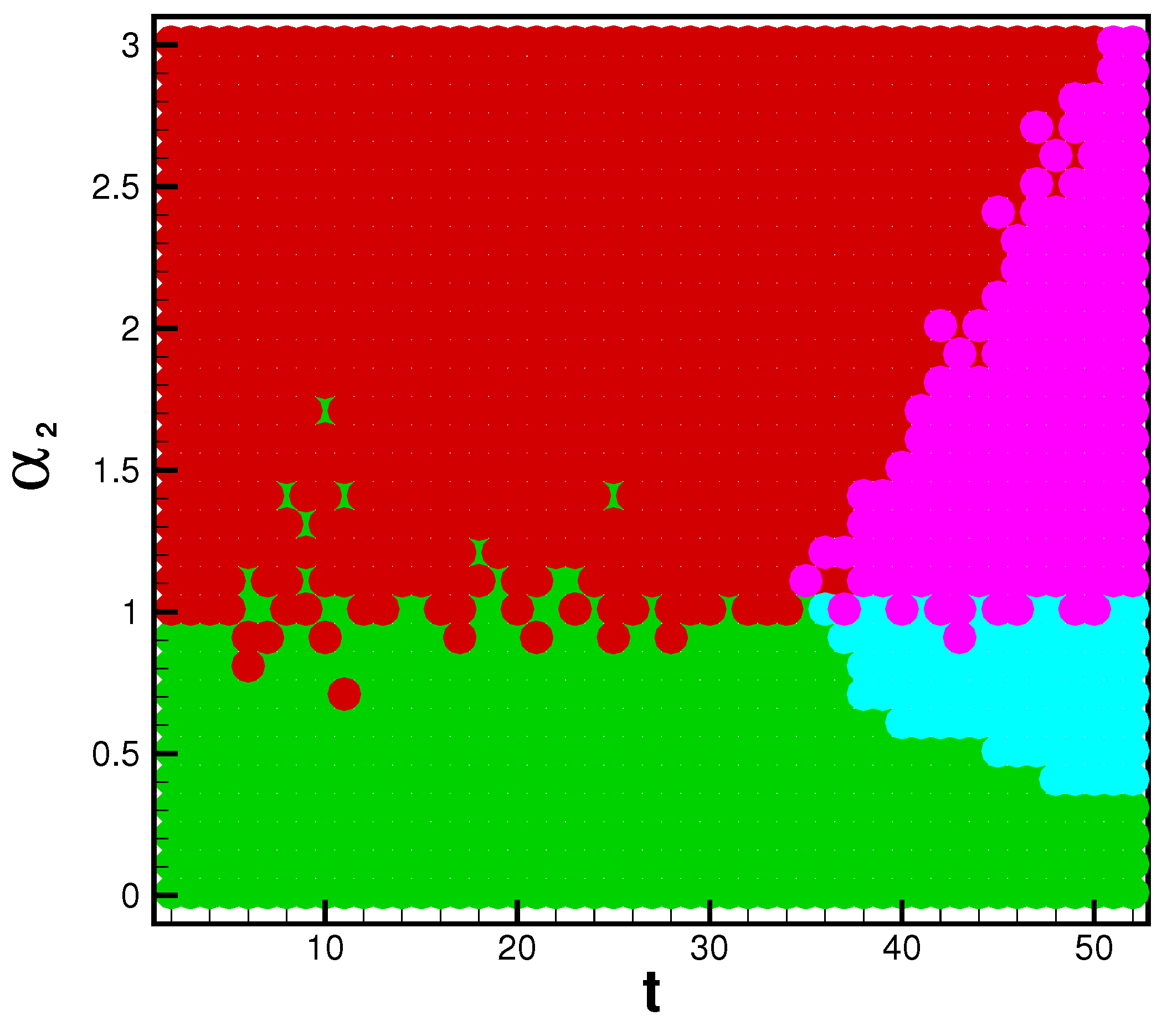
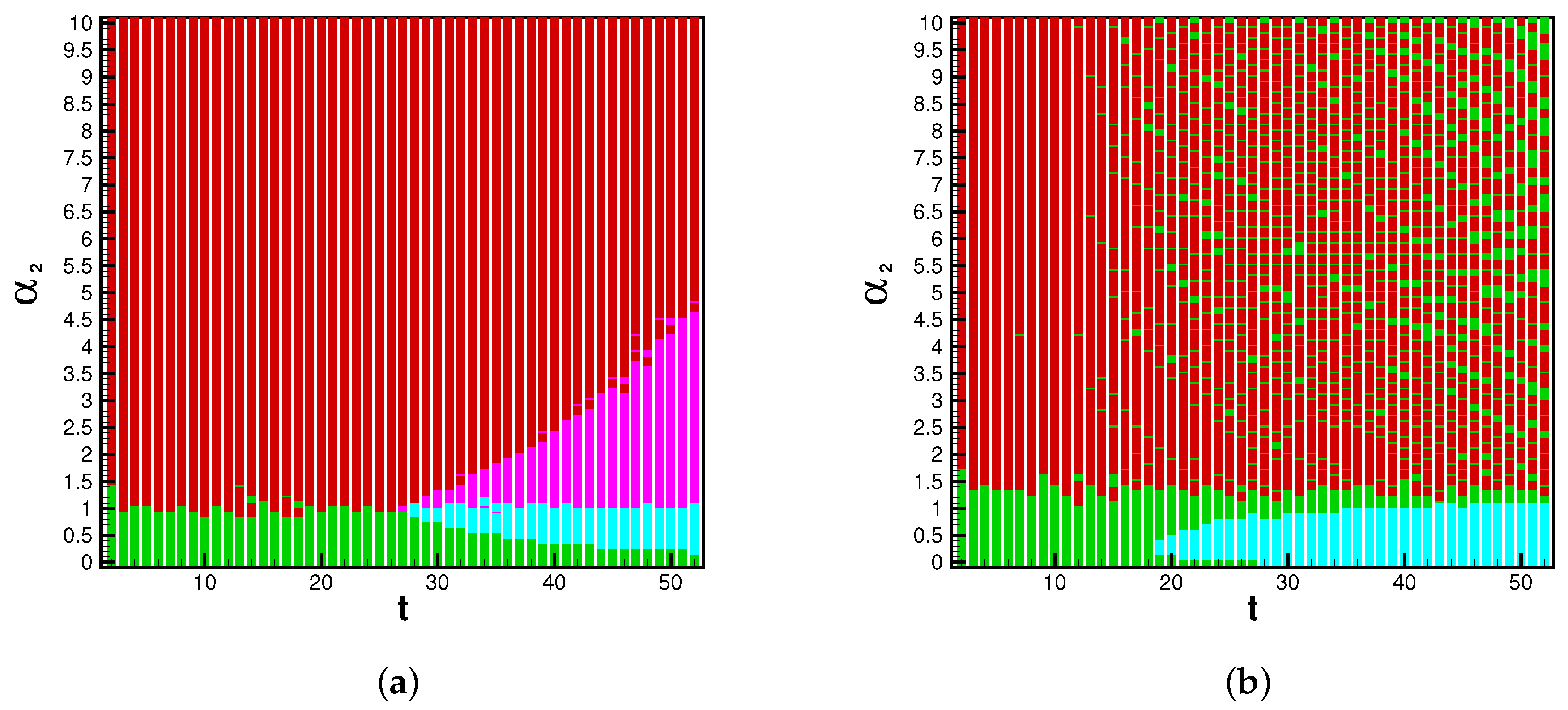
The game analysis can provide insight into strain dominance as a function of time, and viral mutability. Phase diagrams inform the payoff matrix, which tells us the parameter range for which a strain becomes dominant. In the influenza cases, the system is strongly biased toward Type A flu. For this reason we see the A pathway and AB pathway dominant in the beginning of each season. When enough time has passed, and mutability is high enough, the B and BA pathways may gain dominance. With the eventuality of reliable rates for each strain of SARS-CoV-2, this infection pathway analysis will be valuable for determining the danger of emerging strains. The possible system’s states are illustrated by a phase space, dependent upon the position in time (t) of the flu season and the value of the mutability parameter ${\alpha }_2$. The dominant pathway is calculated with each combination of parameters. The A-pathway is dominant if Type A infections > Type B infections and Type B infections $<0.00001$. The BA pathway is dominant if Type A infections > Type B infections and Type B infections $>0.00001$. The B pathway is dominant if Type A infections < Type B infections and Type B infections $>0.00001$. Finally, the AB pathway is dominant if Type A infections < Type B infections and Type B infections $<0.00001$. The threshold $0.00001$ is chosen because, on average during the 2015 influenza season, $0.00001\%$ of the NYC population was infected by Type B influenza; this is universally lower than Type A influenza. In applications of this model toward the SARS-CoV-2 virus, we could reasonably expect this threshold to be lower or nonexistent, as emerging strains have shown the ability to become dominantly infectious. ${\alpha }_2$ and t determine the bridge pathways’ dominance if Type B cases are above or below the threshold. Thus, for any flu season, a payoff matrix is determined by the duration of spread and the value of a viral strain’s mutability, as seen in

Table 2. The table shows the dominant pathways for given choice of time and mutability. Estimations for the conditionals are based on the general shape of the phase diagram. Most notably, ${\alpha }_2$ has a noticeable switch at about ${\alpha }_2=1$, while the time at which a pathway switch occurs is based on the magnitude of ${\alpha }_2$. The equations shown as column headers are best-fit curves for the borders of red/purple and green/cyan.

	$\mathit{t}<-28.33\left({\mathit{\alpha }}_2\right)+63.33$	$\mathit{t}>94.79{\left({\mathit{\alpha }}_2\right)}^2-155.51\left({\mathit{\alpha }}_2\right)+98.75$
${\alpha }_2>1$	AB-pathway	B-pathway
${\alpha }_2<1$	A-pathway	BA-pathway

.

3. Results

$\overline{∆G}$ calculations are performed on individual epidemic spread of Influenza and SARS-CoV-2. $\overline{∆G_I}$ and $\overline{∆G_D}$ are compared to epidemic severity measures such as death and infection counts. Fits are performed for data extracted from New York County, NY. Data are courtesy of Johns Hopkins [1] and the Centers for Disease Control (CDC) [22]. The change in free energy of reaction is examined in three contexts: individual spread, or case studies of of past flu seasons; twindemic forecasting, or theoretic contemporaneous spread of SARS-CoV-2 overlaid with previous flu seasons; multi-strain model, or an application of the scalable multi-strain epidemic model for Type A and Type B influenza.

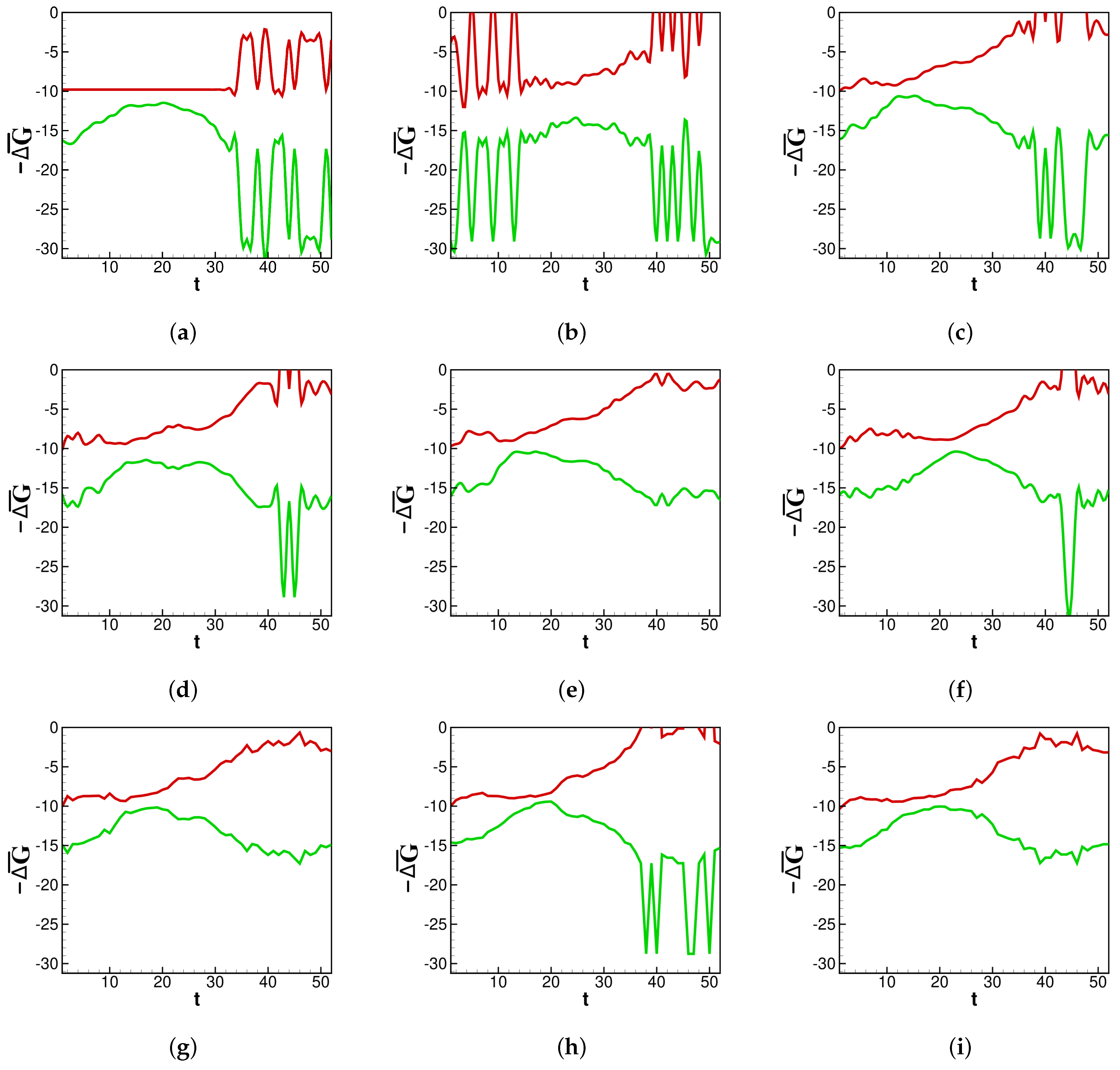
In Figure 2a–i and moving forward, t denotes the number of weeks since the beginning of the influenza season or SARS-CoV-2 spread. First, $\overline{∆G}$ calculations are examined in the context of past flu seasons.

Individual spread: A strong source of model validity will be the thermodynamic analysis on the viral spread for previous flu seasons. The results will be compared to CDC estimates for the “burden” of an individual influenza epidemic. The CDC defines a season’s burden based on confirmed infections and deaths. We present $\overline{∆G}$ values generated by our model through recent flu seasons. Figure 2a–i shows the thermodynamic behavior captured by the rate constants in our fit.

Here, it is shown how the thermodynamic activity between bins behaves during different influenza epidemics. Across each season in Figure 2a–i, a lower number of deaths near the end of each season corresponds to $-\overline{∆G_D}$ becoming less negative. It is generally true that deaths wane at the end of an influenza season, and the same is true for $-\overline{∆G_D}$, which generally increases after the peak of the influenza season. Depicted in Figure 2a–i, around the middle of each season, there is a concave down segment of $\overline{∆G_I}$ corresponding to a peak in new infections. $\overline{∆G_I}$ provides a pre-severity measure: spontaneity is highest as infections grow, and lowest when infections peak and subsequently begin to die out. Some flu seasons with a multimodal distribution of infections, such as in 2013 (Figure 2d), contain an inflection point in their concave down section of $\overline{∆G_I}$. This is another pre-severity measure. $\overline{∆G_I}$ returns to the baseline just before the new season is set to begin. One can imagine the rightmost side of panel (a) connecting to the leftmost edge of panel (b) as data for new infections are collected continuously from year to year. The same is not true for $\overline{∆G_D}$ because the death counts reset each flu season. Spikes in both $\overline{∆G_I}$ and $\overline{∆G_D}$ are artifacts of weeks near the beginning or end of an infectious season reporting zero new infections. For the purposes of data smoothing to avoid computational singularities, we estimate zero infections to be equal to ${10}^{-7}$ new infections. Nevertheless, the change in magnitude helps illustrate how $∆G$ is sensitive to sudden changes in concentrations.

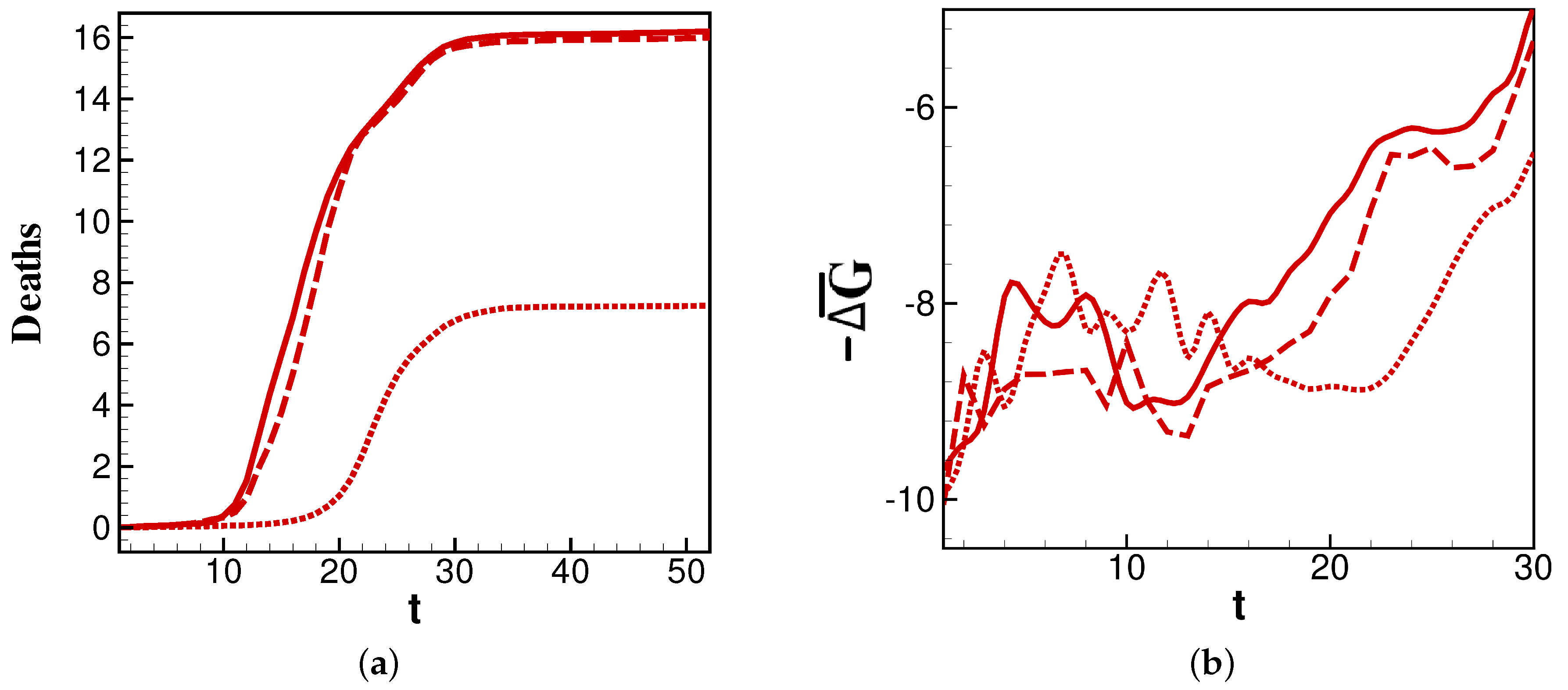
We further examine $\overline{∆G_D}$ values for the 2014, 2015, and 2016 flu seasons as an interesting change in burden that occurs in these sequential years. Figure 3a shows that the years 2014 and 2016 have similar profiles, while 2015 has a later and less-burdensome death count. This is reflected in Figure 3b, where $-\overline{∆G_D}$ for each year is minimal just before the steepest point of its corresponding deaths curve. The correlation is most apparent in the delayed time for $-\overline{∆G_D}$ in 2015 to reach the minimum. Thus, the comparison of 2014 and 2016 to 2015 in Figure 3 affords two important conclusions: the overall burden of a year’s infections correlate to the persistence of relatively highly negative $-\overline{∆G_D}$ values, and the timing of peak burden tracks closely with the minimum of $-\overline{∆G_D}$.

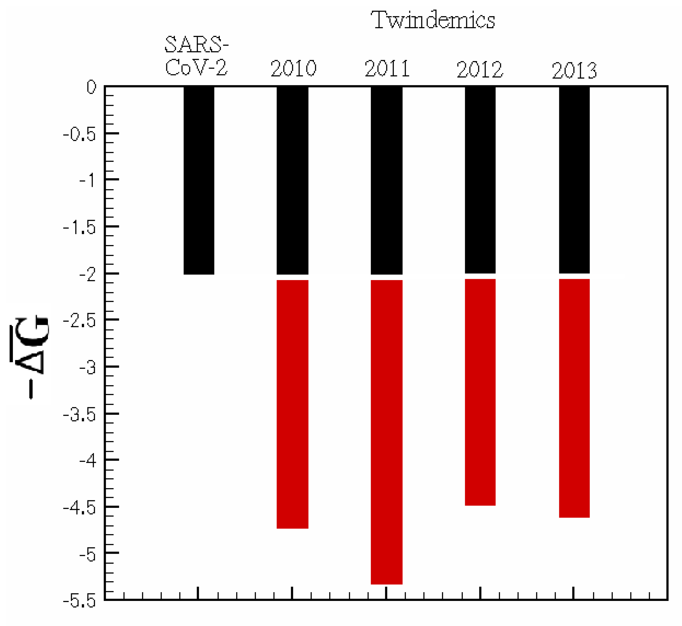
Twindemic forecasting: By taking rate constants derived from individual spread dynamics, we apply those constants to initial conditions based on the current population to understand how the interplay of two viral pathways might give rise to an increase in network thermodynamic activity, measured by $∆G$. In compartmental models, network thermodynamics can answer the question: does the existence of two distinct viral pathways increase the activity along the branches of a compartmental epidemiological network? In other words, is a twindemic’s burden greater than the sum of its viral parts? The answer to this question could have implications in the future of SARS-CoV-2 and influenza twindemics and the rising threat of quickly mutating respiratory viruses.

We examine the effects of adding a second viral pathway on the baseline of $\overline{∆G_{I_c}}$. We sample the data from the first months of the SARS-CoV-2 outbreak in NYC and overlay those data with a small sample of our previously explored flu seasons from 2010 to 2014 during peak infectiousness. For each season studied in Figure 4, any parallel viral pathway increases the infectious thermodynamic activity of a viral outbreak. Hence, the methods proposed are valuable in predicting the future interplay of SARS-CoV-2 and seasonal influenza and how this interplay affects disease burden.

For the 2020–2021 flu season, these predictions would be difficult because of the collateral effects that mitigation efforts, such as masking, distancing, and lockdowns, have produced. However, as data become more widely available, periods of time where intervention techniques were mandated can be compared to non-mandated regions or time frames to further infer the effect of imposed mitigation. Further thermodynamic investigation of SARS-CoV-2 variants could help understand the stability of novel mutations and their infectious pathways. Quantifying the conception that the kinetic implications of multi-pathway viral epidemics can contribute to increased infectiousness may help reconcile the boom of cases found around SARS-CoV-2 variants.

Multi-strain model: Finally, a model based on emergent strains is studied. An exploration toward the efficacy of this model is performed based on the Type A and Type B influenza seasons beginning in 2015. This season is chosen for an ample distribution of both Type A and Type B influenza. As before, data fits are performed for infection and death rates: ${\beta }_A$ and ${\delta }_A$ for Type A and ${\beta }_B$ and ${\delta }_B$ for Type B. This modeling paradigm then introduces rates along a bridge between infectious categories that is interpreted as mutability between strains. Here, ${\alpha }_1$ is the likelihood of Type B mutating to Type A, and ${\alpha }_2$ is Type A mutating to Type B. In the emerging strain model, ${\alpha }_1$ is set to 1 by normalization and we exert control on virus mutability by varying ${\alpha }_2$ from 0 to 3. By employing a game-theoretic analysis of pathway domination [15] we determine the dominant infectious pathway throughout an entire influenza season as a function of ${\alpha }_2$. Essentially, we classify dominant pathways by comparing the dynamic concentrations of each compartment.

The dynamics of a viral epidemic in the emergent strain model will rely heavily upon the chosen mutability parameter. The A pathway to infection is dominant with sufficiently low ${\alpha }_2$ Conversely, the B pathway is dominant with sufficiently high values of ${\alpha }_2$. In between, there are critical values of ${\alpha }_2$ where pathway switching occurs. In context, this phase diagram shows the emergence of potentially more dangerous strains. Based on known mutability and epidemic length, the phase diagram and payoff matrix offer insight into when controls of spread should be established.

These figures inform the payoff matrices, seen in Table 2, which displays the parameter range for which a strain becomes dominant. In the influenza cases, the system is strongly biased toward Type A flu. For this reason, we see the A pathway and AB pathway being dominant in the beginning of each season. When enough time has passed, and mutability is high enough, the B- and BA pathways may gain dominance. With the eventuality of reliable rates for each strain of SARS-CoV-2, this infection pathway analysis will be valuable for determining the danger of emerging strains. The reason we choose to present the 2015 season in the main study is because Type B flu has substantially many infections such that it can become dominant. In 2016, Type-A contains a larger majority of infections, thus the B-pathway is not likely to become dominant.

Ultimately, we will examine the executable control on the multi-strain model through the mutability rates. We will generate values for infections and $∆G$ for viral pathways with various levels of ${\alpha }_2$.

With mutability rates set to zero, the multi-strain model reverts to a standard SIR-type model. A dominance of Type-A infections, which agrees with actual influenza spread for 2015, is observed in row one of

Table 3. The table shows the non-dimensional difference in maximum new cases of Type B and Type A influenza, and the stability of each pathway. The first row is the control model, with no bridge rates defined. Each successive row increases the mutability of the Type-A to Type-B mutation.

$\frac{{\mathit{\alpha }}_2}{{\mathit{\alpha }}_1}$	${\mathit{B}}_{\mathit{inf}}-{\mathit{A}}_{\mathit{inf}}$	$\overline{\mathbf{\Delta }{\mathit{G}}_{\mathit{A}}}<0$	$\overline{\mathbf{\Delta }{\mathit{G}}_{\mathit{BA}}}<0$	$\overline{\mathbf{\Delta }{\mathit{G}}_{\mathit{B}}}<0$	$\overline{\mathbf{\Delta }{\mathit{G}}_{\mathit{AB}}}<0$
${\alpha }_1={\alpha }_2=0$	−0.0109	Yes	No	Yes	No
1	−0.00351	Yes	Yes	Yes	Yes
$1.5$	0.0104	Yes	Yes	Yes	Yes
$1.75$	0.0115	Yes	Yes	Yes	Yes
2	0.0107	Yes	Yes	Yes	Yes

. Further, when mutability parameters are set to zero, we notice that the two mutation pathways, $AB$ and $BA$, are not stable. When mutability parameters are introduced, all pathways in the multi-strain model become stable. With $\frac{{\alpha }_2}{{\alpha }_1}>1$, $B_{inf}$ overtakes $A_{inf}$. In other words, with sufficiently high mutability, a new strain can become dominant. The difference in infections supports the conclusions drawn by the dominant pathway phase plane in Figure 5 and Figure 6.

It is worth noting that this method can be extrapolated to study the various subtypes of Type A influenza and/or notable variants, such as H1N1, which are more intimately genetically related. Most importantly, this model is primed for a study of the SARS-CoV-2 virus and its many variants.

4. Discussion

The main goal of this paper is to bring network science and non-equilibrium thermodynamics (i.e., network thermodynamics) along as tools into model-based epidemiology. To such ends, we answer three main questions:

Q1 :

What is the novel utility of the multi-strain model?

Q2 :

Why is ∆G a good metric for characterizing infectious activity and a tool for analyzing emergent strains?

Q3 :

How can the multi-strain model be used in the future for SARS-CoV-2 and other highly mutable viruses?

The utility of the models presented here is chiefly to open the compartmental epidemiology to network thermodynamics and allows for the investigation of highly complex problems. First, human behavior is not easily categorized and is certainly far from the thermodynamic equilibrium; the same applies to the way that diseases spread. By adding pathways to the model, we aim to distribute the model parameters in a way that more accurately captures the complex organization of epidemiological systems. The modification of the standard SIR-type models is motivated by the onset of SARS-CoV-2 and the danger of highly mutable respiratory viruses. As the model dimension grows and complexity increases, tools of non-equilibrium thermodynamics help us draw stronger conclusions about the emergent adaptation of the system to control parameters. $∆G$ can identify the stability of pathways in large networks, while the game-theoretic framework quantifies the dominance of a particular strain.

$∆G$ is a valuable tool in analyzing this network approach to model-based epidemiology. Compartmental models are mass-action based, thus giving us access to a population’s effective concentration and inter-compartmental rates of transfer. These components create a direct analogy to the utility of free energy computations in chemistry. The directed nature of these networks allows us to discuss the chemical properties of $∆G$, such as spontaneity and stability in the context of infectious activity and emergent strains. 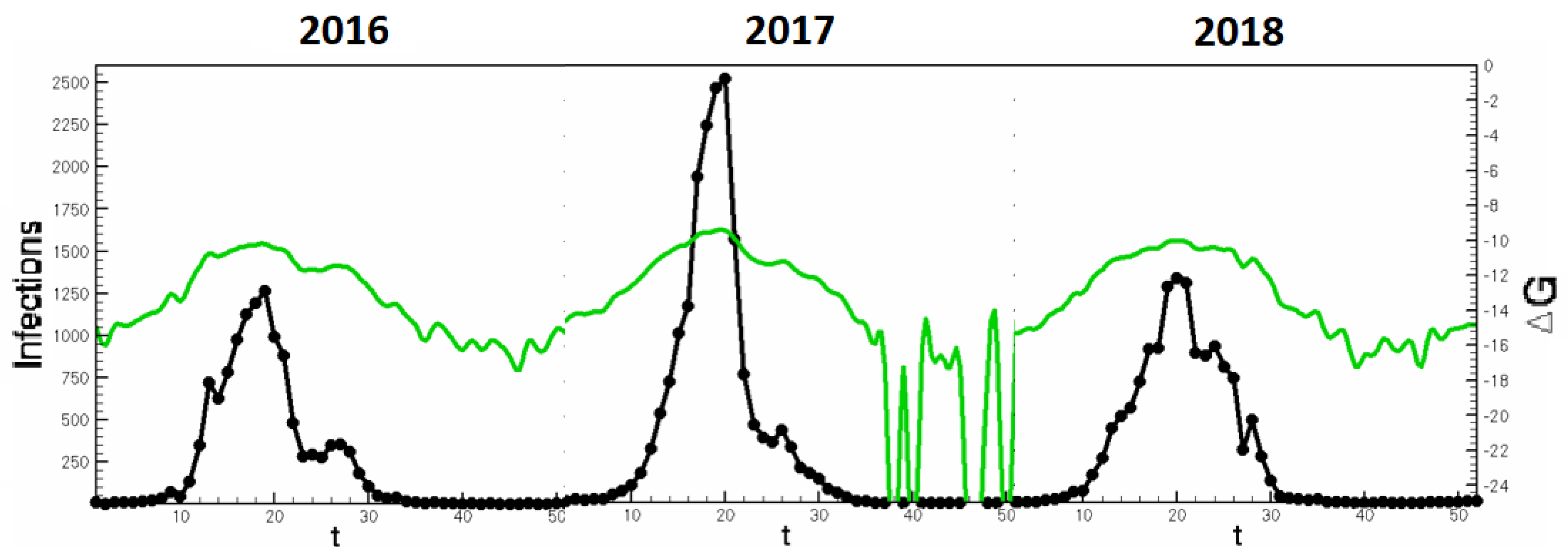The multi-strain approach in Section 3 could be adapted to seasonal studies in order to ascertain seasonal occurrence of emergent strains. In Figure 7, concurrent Influenza seasons are stitched to display the continuity of $∆G$ and infection counts. Such analyses allow a predictive tool for peak infectiousness across seasons.

In the context of the multi-strain model, this analysis can show the emergence of new dominant strains as in the toy model shown in Table 3. The progression of emergent strains can be seen in the rows of the table. When mutability increases, bridge pathways between strains become stable and the difference of B infections to A infections becomes closer to zero. Then as mutability further increases, B infections become larger than A. Thus it is possible to create an automatic alert system which signifies the spontaneity of new viral pathways to infection. With contemporary data on strain-differentiated infections, one can note the changing spontaneity of bridge pathways and infection counts in real time and before emergent strains gain dominance, triggering alerts and advising intervention strategies. Therefore, $∆G$ serves as an indicator of emerging paths—before they are destructively widespread—and arms policy makers with early warning signs. Further, considering many virus and host-dependent factors contributing to mutability [37], a study of large phase spaces as shown in Figure 5 illuminates the large number of possible states in the viral landscape.

Furthermore, the $∆G$ equation contains physical parameters (such as temperature), which can abstract “seasonal” components to viral spread. For example, high T⇒ high $∆G$⇒ high spontaneity. Thus, T is a controllable parameter which can increase or decrease infectious spontaneity. This controllability can open $∆G$ as a metric for informing intervention methods. For example, lockdowns and social distancing would mean low T, which reduces spontaneity. This correlates with the fact that lockdowns reduce infections. This is one way of using $∆G$ for creating informative intervention tools.

Finally, the use of complex lumped parameter networks will help us build models which accurately describe quickly mutating epidemics. The switching dynamics of viruses which can change characteristics quickly is not captured by standard SIR-type models. Instead, the multi-strain model can illuminate the nuances of strain emergence by defining switching parameters. Equations (10)–(12) and Algorithms 1–4 present a framework for which complex networks of mutable pathogens can be built. This is one direction in which epidemiological models could move toward to better understand SARS-CoV-2 and its variants.

5. Conclusions

In addition to the novel utility of the models proposed, we provided some examples of their efficacy. First, we use change in free energy ($∆G$) computations to show how infectiousness corresponds to the spontaneity measure of $∆G$, i.e., we show how rising deaths during past flu seasons correspond to a change in magnitude for $∆G$ in Figure 3a,b.

Second, we explore a model where two viruses spread contemporaneously. By examining $∆G$, the twindemic model shows how two viral interplaying pathways can be more burdensome than a simple sum of parts. In other words, $∆G$ highlights how the nuance of the relationship between connected populations can be captured by employing network thermodynamics in high order compartmental models.

Third, we present the multi-strain model as a framework for modeling highly mutable epidemics. This is particularly aimed toward modeling SARS-CoV-2 and its variants with a properly complex model. A case study in Type A and Type B influenza shows the efficacy of the multi-strain model for modeling related viral strains. Particularly for future compartmental models with high complexity, where dynamic quantities are difficult to relate, $∆G$ identifies the stability of extended pathways in large networks, while the game-theoretic framework quantifies a certain mutation’s dominance.

We considered many future directions of this work when formulating our models. One limitation of our study is the simplicity of the underlying SIR-type model. Future work in the area of SARS-CoV-2 can include more fine-tuned models, such as SEIRD models. Further, spatial mobility models could make an improvement in the case of SARS-CoV-2, where geography plays an important role. Most importantly, the multi-strain model is scalable to any number or type of compartments. Thus, the multi-strain model is ripe for optimization techniques which can uncover the most effective modeling paradigm. This application is not only important to the current applications, but toward an automatic model complexity selection process in general.