Article

A Discrete Exponential Generalized-G Family of Distributions: Properties with Bayesian and Non-Bayesian Estimators to Model Medical, Engineering and Agriculture Data

by
Mohamed S. Eliwa
1,2,4,*,
Mahmoud El-Morshedy
3,4 and
Haitham M. Yousof
5
1
Department of Statistics and Operation Research, College of Science, Qassim University, Buraydah 51482, Saudi Arabia
2
Section of Mathematics, International Telematic University Uninettuno, I-00186 Rome, Italy
3
Department of Mathematics, College of Science and Humanities in Al-Kharj, Prince Sattam Bin Abdulaziz University, Al-Kharj 11942, Saudi Arabia
4
Department of Mathematics, Faculty of Science, Mansoura University, Mansoura 35516, Egypt
5
Department of Statistics, Mathematics and Insurance, Benha University, Benha 13518, Egypt
*
Author to whom correspondence should be addressed.
Mathematics 2022, 10(18), 3348; https://doi.org/10.3390/math10183348
Submission received: 2 August 2022 / Revised: 30 August 2022 / Accepted: 9 September 2022 / Published: 15 September 2022
(This article belongs to the Special Issue Current Developments in Theoretical and Applied Statistics)

Abstract

:
This paper introduces a new flexible probability tool for modeling extreme and zero-inflated count data under different shapes of hazard rates. Many relevant mathematical and statistical properties are derived and analyzed. The new tool can be used to discuss several kinds of data, such as “asymmetric and left skewed”, “asymmetric and right skewed”, “symmetric”, “symmetric and bimodal”, “uniformed”, and “right skewed with a heavy tail”, among other useful shapes. The failure rate of the new class can vary and can take the forms of “increasing-constant”, “constant”, “monotonically dropping”, “bathtub”, “monotonically increasing”, or “J-shaped”. Eight classical estimation techniques—including Cramér–von Mises, ordinary least squares, L-moments, maximum likelihood, Kolmogorov, bootstrapping, and weighted least squares—are considered, described, and applied. Additionally, Bayesian estimation under the squared error loss function is also derived and discussed. Comprehensive comparison between approaches is performed for both simulated and real-life data. Finally, four real datasets are analyzed to prove the flexibility, applicability, and notability of the new class.

1. Introduction

The discretization of current continuous models has recently drawn significant interest. This is due to the fact that the data must often be recorded on a discrete scale rather than a continuous analog. Examples include the number of daily COVID-19 deaths, or the number of renal cysts caused by steroid use, among others. In order to discuss such data, new discrete models have been proposed and investigated in the statistical and mathematical literature. For instance, the discrete Weibull (DW) (Nakagawa and Osaki [1]), discrete Rayleigh (DR) (Roy [2]), discrete inverse Weibull (DIW) (Jazi et al. [3]), discrete exponential (DE) (Gomez-Déniz [4]), discrete inverse Rayleigh (DR) (Hesterberg [5]), discrete exponentiated Weibull (EDW) (Nekoukhou and Bidram [6]), discrete Lindley-II (DLy-II) (Hussain et al. [7]), discrete Lomax (DLx) and discrete Burr XII (DBXII) (Para and Jan [8]), discrete generalized Burr–Hatke distribution (for more details, see El-Morshedy et al. [9]), discrete exponentiated Lindley (EDLy) (see El-Morshedy et al. [10]), discrete generalized Burr–Hatke distribution (see Yousof et al. [11]), and the discrete inverse Burr (DIB) distribution (see Chesneau et al. [12]), among others.
On the other hand, another statistical approach has recently been followed up to define new discrete G families of probability distributions. The statistical approach depends on generating new discrete G families of probability distributions based on some existing continuous families. For example, following Bourguignon et al. [13], Aboraya et al. [14] defined and studied the discrete Rayleigh G (DR-G) family of distributions, while Ibrahim et al. [15] proposed a discrete analog of the Weibull G family. Following Steutel and van Harn [16], Eliwa et al. [17] introduced and discussed the discrete Gompertz G (DGz-G) family of distributions. Recently, Yousof et al. [18] presented a new G family of continuous distributions called the exponential generalized G (EG-G) family. The CDF of the EG-G family can be expressed as follows:
F α , γ z = 1 e x p O z ; γ , ξ   | z R   and   α , γ > 0 ,
where
O z ; γ , ξ = G ˙ ξ γ z 1 | z R , γ > 0 ,
is the generalized odds ratio argument, G ˙ ξ z = 1 G ξ z refers to the survival function (SF) of any baseline model with the parameter vector ξ , α is a scale parameter, and γ is an additional shape parameter. In this work and following Yousof et al. [18] and Steutel and van Harn [16], we define and study a new discrete analog of the EG-G family called the discrete exponential generalized G (DEG-G) family. We are motivated to introduce the DEG-G family for the following reasons:
  • Generating new probability mass functions that can be “asymmetric and left skewed”, “asymmetric and right skewed”, “symmetric”, “symmetric and bimodal”, “uniformed”, or “right skewed with a heavy tail”, among other useful shapes. The wide flexibility of the probability mass function (PMF) for any new model allows us to employ the new model for analyzing many different environmental datasets.
  • Presenting some new special models with different types of hazard rate functions (HRFs), such as “increasing-constant”, “constant”, “monotonically decreasing”, “bathtub”, “monotonically increasing”, “decreasing–increasing-decreasing”, and “J-shaped”. The more forms of failure rates, the greater the elasticity of the distribution. These shapes facilitate the work of many practitioners, who may use the new distribution in statistical modeling and mathematical analysis. For this specific purpose, we give the problem of checking the failure rate function a great deal of attention.
  • The degrees of the skew coefficient, kurtosis coefficient, failure rate function, and diversity in the PMF and failure rate functions all play a role in the flexibility of the new distribution. Additionally, the probability distribution’s usability and effectiveness in statistical modeling are crucial in this regard. Examining the novel PMF, we discovered that it was quite adaptable in this and other areas. This is what motivated us to investigate this probability distribution thoroughly.
  • Proposing new discrete models for modeling “over-dispersed”, “equal-dispersed”, and “under-dispersed” real data. As shown in this paper, the new discrete family has shown a remarkable superiority in modeling these types of data, whether symmetric or asymmetric, and containing outliers or not containing outliers.
  • Introducing new discrete models for analyzing extreme and zero-inflated count data.
  • Comparison of the estimation methods with both simulated and real-life data for recommending the best method in each case.
  • A zero-inflated probability distribution, or distribution that permits many zero-valued observations, is the foundation of a statistical model known as a zero-inflated model in statistics. For instance, individuals who have not purchased insurance against the risk, and are therefore unable to make a claim, would cause the quantity of insurance claims within a community for a particular type of risk to be zero-inflated. Often, the zero-inflated Poisson regression model is used for modeling and predicting the zero-inflated count data; however, in this paper, we are motivated to use the DEG-G family for this purpose.
  • In statistical modeling of the bathtub hazard rate count data, the DEG-G family under the Weibull baseline model provides adequate results; hence, the DEG-G family under the Weibull baseline is recommended for modeling the bathtub hazard rate count data (see Section 6.1). Moreover, the same baseline model is also suitable for modeling the monotonically increasing failure rate count data with adequate fitting (see Section 6.2).
  • In the case of zero-inflated medical data with a decreasing failure rate and some outliers, the new family is an appropriate choice to deal with this type of data (see Section 6.3).
  • In case of zero-inflated agricultural data with a decreasing–increasing–decreasing failure rate and some outliers, the new class is an appropriate choice for modeling this kind of data (see Section 6.4).
  • In fact, we empirically demonstrate that the proposed family of distributions fits four real datasets more accurately than 16 other extended relevant distributions with 3–4 parameters (see Section 7).
  • Through simulation experiments and relying on the new class, many of the classical estimation techniques and Bayesian approaches are tested and evaluated, and important conclusions are reached in this regard, including the following:
The maximum likelihood estimation approach is still the most efficient and most consistent of the rest of the classical methods; however, most of the other methods perform well, except for the Kolmogorov estimation method.
  • Generally, the Bayesian technique and maximum likelihood estimation method can be recommended for statistical modeling and applications.
  • The Kolmogorov estimation method provides the worst results for all real datasets; this problem still needs more investigation for understanding of its main reasons.
Many helpful statistical properties, such as the probability-generating function, central and ordinary moment, moment-generating function, cumulant-generating function, and dispersion index (Disp-Ix), are calculated and statistically examined in this article once the new generator is defined. Some special discrete members, based on Weibull (W), inverse Weibull (IW), Lomax (Lx), Burr X (BX), inverse Burr X (IBX), log-logistic (LL), Rayleigh (R), inverse Rayleigh (IR), exponential (E), inverse Lindley (ILi), inverse Lomax (ILx), inverse log-logistic (ILL), inverse exponential (IE), and Lindley (Li) distributions, are listed in Table 1. Different classical (non-Bayesian) methods of estimation, including the Cramér–von Mises estimation (CVME), maximum likelihood estimation (MLE), ordinary least squares estimation (OLSE), bootstrapping (Bootst), L-moments (L-mom), Kolmogorov estimates (KE), weighted least squares estimation (WLSE), and Anderson–Darling left-tail from the second order (AD2LE), are considered. For more details about these methods, see the works of Chesneau et al. [12], Yousof et al. [18], Aboraya et al. [14], and Ibrahim et al. [15]. The Bayesian estimation under the squared error loss function is also considered. The well-known Markov chain Monte Carlo (MCMC) simulations are performed to compare the classical and Bayesian methods. The applicability of the DEG-G family is explained and discussed using four real-life datasets. The DEG-G family under the Weibull model case provides a more adequate fit than many competitive models, due to the consistent Akaike information criterion (CAICR), Akaike information criterion (AICR), chi-squared ( χ V 2 ), Kolmogorov–Smirnov (K–S), and corresponding p-value (P.V). For more detail about these statistics, see the works of El-Morshedy et al. [9,10], Aboraya et al. [14], and Eliwa et al. [17].

2. The DEG-G Class

Starting with (1) and utilizing the discretization approach, the CDF of the DEG-G family can be formulated as follows:
F W z = 1 p O z + 1 ; γ , ξ   | p I = 0 , 1   and   z N 0
where W = ( p , γ , ξ ), e x p α = p , N 0 = N 0 and
O z + 1 ; γ , ξ = 1 G ξ z + 1 γ 1 = G ˙ ξ γ z + 1   |   z N 0 .
The corresponding SF to (2) can be derived as follows:
F ¯ W z = p O z + 1 ; γ , ξ   | p I   and   z N 0 .
According to Kemp [19] and (3), the PMF of the DEG-G family can be expressed as follows:
f W z = F ¯ W z 1 F ¯ W z ,
where
f W z = p O z ; γ , ξ p O z + 1 ; γ , ξ   | p I   and   z N 0 .
Based on (3) and (4), the hazard rate function (HRF) can then be proposed as follows:
H W z = f W z / F ¯ W z 1 = 1 p O z ; γ , ξ p O z ; γ , ξ p O z + 1 ; γ , ξ .
In Table 1, some members of the DEG-G family are provided. The new PMF in (4) is most tractable when the CDF of the baseline member G ξ z has a simple analytic expression.
For the W model, we have O z ; γ , ξ = e x p γ z θ 1 1 | γ , θ > 0 . Then, based on (3), the PMF of the DEGW model can be expressed as follows:
f W z = p e x p γ z θ 1 p e x p γ z + 1 θ 1   | z N 0 , p I   and   γ , θ > 0 .
In Figure 1 and Figure 2, some PMF and HRF plots of the DEGW model are sketched under some selected parameter values. Based on Figure 1, it can be seen that the PMF of the DEGW can be “asymmetric and left skewed”, “asymmetric and right-skewed”, “symmetric”, “uniform”, or “right-skewed with heavy tail”, among other useful PMF shapes. Moreover, it can be used as a probability tool to discuss zero-inflated data. According to Figure 2, we can conclude that the HRF of the DEGW can be “increasing-constant”, “constant”, “monotonically decreasing “, “bathtub or decreasing-constant-increasing “, “monotonically increasing”, or “J-shaped”.

3. Main Properties

3.1. Moments

 Theorem 1. 
Z is a non-negative random variable (RV), where Z DEG-G ( W ) family, then the rth moment of the RV Z can be expressed as follows:
μ r , Z = E Z r = z = 1 + z r z 1 r p O z ; γ , ξ | z N 0 , p I   and   r = 1 , 2 , 3 , .
 Proof. 
Since
μ r , Z = E Z r = z = 0 + z r f W z .
then,
μ r , Z = E Z r = z = 0 + z r p O z ; γ , ξ p O z + 1 ; γ , ξ = z = 1 + z r z 1 r F ¯ W z 1 .
Thus,
μ r , Z = z = 1 + z r z 1 r p O z ; γ , ξ | z N 0 , p I   and   r = 1 , 2 , 3 , .
Using (5), the mean μ 1 , Z , μ 2 , Z , μ 3 , Z , μ 4 , Z , and variance ( V Z ), can be respectively written as follows:
μ 1 , Z = μ 1 , Z = E Z = z = 1 + p O z ; γ , ξ | z N 0 , p I   and   r = 1 ,
μ 2 , Z = E Z 2 = z = 1 + 2 z 1 p O z ; γ , ξ | z N 0 , p I   and   r = 2 ,
μ 3 , Z = E Z 3 = z = 1 + z 3 z 1 3 p O z ; γ , ξ | z N 0 , p I   and   r = 3 , ,
μ 4 , Z = E Z 4 = z = 1 + z 4 z 1 4 p O z ; γ , ξ | z N 0 , p I   and   r = 4
and
V Z = z = 1 + 2 z 1 p O z ; γ , ξ z = 1 + p O z ; γ , ξ 2 | z N 0 , p I   and   r = 2 .
Table 2 lists some numerical results for μ 1 , Z , μ 2 , Z , μ 3 , Z , and μ 4 , Z under the DEGW model. It should be noted that the first four moments can be numerically evaluated, although they have no closed forms. All numerical results in Table 2 were derived using the R program, and the infinity problem was overcome by assuming a very large value instead of it (108), since values beyond this value can be ignored because they are too small. Therefore, the results of μ 1 , Z , μ 2 , Z , μ 3 , Z , and μ 4 , Z are approximated.

3.2. Central Moment and Dispersion Index

The r t h central moment of the RV Z , i.e., μ r , Z , can be formulated as follows:
μ r , Z = E ( Z μ r , Z ) r = ω = 0 r μ 1 , Z ω r ω μ r ω | | z N 0 , p I   and   r = 1 , 2 , 3 , .
Hence, the V ( Z ) can be expressed as follows:
E ( Z μ r , Z ) 2 = μ 1 , Z ω = 0 2 μ 1 , Z ω 2 ω μ 2 ω , Z | | z N 0 , p I   and   r = 2 ,
or
μ 2 , Z = V Z = μ 2 , Z μ 1 , Z 2 = z = 1 + 2 z 1 p O z ; γ , ξ z = 1 + p O z ; γ , ξ 2 | z N 0 , p I   and   r = 2 .
The dispersion index (Disp-Ix) of the DEG-G family can derived as follows:
Disp - Ix Z = z = 1 + 2 z 1 p O z ; γ , ξ z = 1 + p O z ; γ , ξ   z = 1 + p O z ; γ , ξ | z N 0   and   p I .
Some numerical results for the Disp-Ix Z are presented in Table 3, with useful comments. The Disp-Ix, also known as the coefficient of dispersion, relative variance, or variance-to-mean ratio (VMR), is a normalized measure of the dispersion of a probability distribution that is used in probability theory and statistics to determine whether a set of observed occurrences is clustered or dispersed in comparison to a common statistical model. It is described as the variance-to-mean ratio. In order to establish whether the observed real dataset can be modeled using a Poisson process, the Disp-Ix is used to measure whether a particular collection of observations is clustered or dispersed compared to a particular statistical model. When the Disp-Ix for any real dataset is less (greater) than 1, the dataset is referred to as under (over)-dispersed phenomena. Table 3 displays a numerical analysis and its associated computations for the Disp-Ix. The kurtosis, i.e., K Z , and skewness, i.e., S Z , of the RV Z can be obtained from the common relationships. Table 3 reports some numerical results for E Z , V Z , S Z , and K Z of the DEGW distribution. Based on Table 3, it can be seen that E Z increases as p increases, and decreases as γ and θ increase. The S Z     1.053185 , . The K Z ranges from 1.02442 to . The Disp-Ix Z   0 , 1 , or “ > 1 “, or “= 1 “, like the standard well-known Poisson distribution (see Poisson [20]). Thus, the DEGW distribution could be useful in modeling “under-dispersed”, “equi-dispersed”, or “over-dispersed” count data.

3.3. Generating Functions

 Theorem 2. 
Assume that Z is the non-negative RV, where Z DEG-G( W ) class. Then, the moment-generating function (MGF) of the RV Z can be derived as follows:
M r , Z t | z N 0 , p I   and   r = 1 , 2 , 3 , = 1 + z = 1 + e x p t z e x p t z 1 p O z ; γ , ξ .
 Proof. 
The MGF of the non-negative RV Z can be derived as follows:
M r , Z t = z = 0 + e x p t z p O z ; γ , ξ p O z + 1 ; γ , ξ ,
thus,
M r , Z t = 1 + z = 1 + e x p t z e x p t z 1 p O z ; γ , ξ | z N 0 , p I   and   r = 1 , 2 , 3 , .
The first r derivatives of (6), with respect to t at t = 0 , yield the first r moments around the origin, i.e.,
μ r , Z | t = 0   and   r = 1 , 2 , 3 , = E Z r = d r d t r M r , Z t ,
where
μ 1 , Z = E Z = d d t M r , Z t | t = 0 = z = 1 + p O z ; γ , ξ | z N 0 , p I   and   r = 1 ,
μ 2 , Z = E Z 2 = d 2 d t 2 M r , Z t | t = 0 = z = 1 + 2 z 1 p O z ; γ , ξ | z N 0 , p I   and   r = 2 ,
μ 3 , Z = E Z 3 = d 3 d t 3 M r , Z t | t = 0 = z = 1 + 3 z z 1 + 1 p O z ; γ , ξ | z N 0 , p I   and   r = 3 ,
and
μ 4 , Z = E Z 4 = d 4 d t 4 M r , Z t | t = 0 = z = 1 + z 4 z 1 4 p O z ; γ , ξ | z N 0 , p I   and   r = 4 .  
The cumulant-generating function (CGF) is the logarithm of the MGF. Thus, the rth cumulant, i.e., C r , Z , can be derived as C r , Z | t = 0 ,   and   r = 1 , 2 , 3 , = d r d t r log M r , Z t . In this context, we can highlight some important mathematical results: The 1st cumulant is the mean ( C 1 , Z = μ 1 , Z ). The 2nd cumulant is known as the variance ( C 2 , Z = μ 2 , Z μ 1 , Z 2 = μ 2 , Z ). The 3rd cumulant is the same as the 3rd central moment C 3 , Z = μ 3 , Z 3 μ 2 , Z μ 1 , Z + 2 μ 1 , Z 3 = μ 3 , Z . However, the 4th and higher-order cumulants are not equal to central moments. The cumulants can be also expressed as follows:
C r , Z | r 1 = μ r , Z ω = 0 r 1 r 1 ω 1 μ r ω , Z C ω , Z .
It is possible to derive the probability-generating function (PGF) as follows:
P Z s = 1 + z = 1 + 1 1 s s z p O z ; γ , ξ | z N 0 , p I   and   r = 1 , 2 , 3 , .

4. Estimation and Inference

In this section, we are concerned with the different estimation methods, including classical methods and Bayesian methods. The classical methods are many and varied, some of which depend on the theory of maximization, and some of which depend on the theory of minimization. In any case, the classical methods on the whole differ from Bayes’ method in their origin and methodology of estimation, as will be explained in detail in theory and practice. The two subsections of this section cover Bayesian and non-Bayesian estimation techniques. Eight non-Bayesian estimation techniques, including the MLE, CVME, OLSE, WLSE, L-mom., KE, Bootst, and AD2LE methods, are taken into consideration in the first subsection. Then, the Bayesian estimation approach under the well-known squared error loss function (SELF) is taken into consideration in the second subsection.

4.1. Classical Estimation Techniques

4.1.1. The Maximum Likelihood Estimation Method

Maximum likelihood estimation (MLE) is a statistical technique for estimating the parameters of a probability distribution that has been assumed given some observed data. This is accomplished by maximizing a likelihood function to make the observed data as probable as possible given the assumed statistical model. The maximum likelihood estimate is the location in the parameter space where the likelihood function is maximized. Maximum likelihood is a popular approach for making statistical inferences, since its rationale is clear and adaptable.
The derivative test for figuring out maxima can be used if the likelihood function is differentiable. The ordinary least squares estimator, for example, maximizes the likelihood of the linear regression model, allowing the first-order requirements of the likelihood function to be explicitly solved in some circumstances. However, in many cases, it is essential to use numerical techniques to determine the probability function’s maximum. MLE is typically comparable to maximum a posteriori (MAP) estimates under a uniform prior distribution of the parameters from the standpoint of Bayesian inference. MLE is a specific example of an extremum estimator in frequentist inference, with likelihood as the objective function. If we assume a random sample Z 1 ,   Z 2 ,   ,   Z n from the presented class, then the log-likelihood function for the vector W can be given as follows:
l W = t = 0 n l n p O z i , n ; γ , ξ p O z i , n + 1 ; γ , ξ | p I   and   z i , n N 0 .
The l W can then be maximized via statistical programs such as “R”, or by solving the nonlinear system obtained from l W by differentiation. Then, the score vectors
U W = l W / p , l W / γ , l W / ξ j T   | j = 1 , 2 , , p ,
can be easily derived as follows:
l W / p = t = 0 n O z i , n ; γ , ξ p O z i , n ; γ , ξ 1 O z i , n + 1 ; γ , ξ p O z i , n + 1 ; γ , ξ 1 p O z i , n ; γ , ξ p O z i , n + 1 ; γ , ξ ,
l W / γ = t = 0 n O z i , n ; γ , ξ γ p O z i , n ; γ , ξ l n p O z i , n + 1 ; γ , ξ γ p O z i , n + 1 ; γ , ξ l n p p O z i , n ; γ , ξ p O z i , n + 1 ; γ , ξ ,
and
l W / ξ j = t = 0 n O z i , n ; γ , ξ ξ j p O z i , n ; γ , ξ l n p O z i , n + 1 ; γ , ξ ξ j p O z i , n + 1 ; γ , ξ l n p p O z i , n ; γ , ξ p O z i , n + 1 ; γ , ξ | j = 1 , 2 , , p .
Setting
0 = l W p , 0 = l W γ , 0 = l W ξ j ,
and simultaneously solving them produces the MLEs for the DEG-G family parameters. For numerically addressing such problems, the Newton–Raphson algorithm is used.

4.1.2. The Cramér–von Mises Estimation Approach

Consider a random sample Z 1 ,   Z 2 ,   ,   Z n from the proposed generator. Then, the CVME of the parameter vector W ( C W ) can be obtained by minimizing
C W = 1 12 n 1 + i = 1 n F W z i , n ω i , n 1 2 | p I   and   z i , n N 0 ,
with respect to (w.r.t) p ,   γ , and ξ , respectively, where ω i , n 1 = 1 2 n 2 i 1 and
C W = i = 1 n 1 p O z i , n + 1 ; γ , ξ ω i , n 1 2 .
The three nonlinear equations below are then solved to yield the CVME of the parameters p ,   γ , and ξ :
0 = i = 1 n 1 p O z i , n + 1 ; γ , ξ ω i , n 1 ς p z i , n + 1 , W ,
0 = i = 1 n 1 p O z i , n + 1 ; γ , ξ ω i , n 1 ς γ z i , n + 1 , W ,
and
0 = i = 1 n 1 p O z i , n + 1 ; γ , ξ ω i , n 1 ς ξ j z i , n + 1 , W ,
where
ς p z i , n + 1 , W = F W z i , n / p ,
ς γ z i , n + 1 , W = F W z i , n / γ ,
and
ς ξ j z i , n + 1 , W = F W z i , n / ξ j ,
are the first derivatives of the CDF of DEG-G distribution w.r.t p ,   γ , and ξ j , respectively.

4.1.3. The Ordinary Least Squares Technique

Geometrically, this is defined as the total of the squared distances between each data point in the set and its corresponding point on the regression surface, which are measured parallel to the axis of the dependent variable. The lower the differences, the better the model fits the data. Particularly in the case of a basic linear regression, when there is only one regressor on the right-hand side of the regression equation, the resultant estimator can be stated by a straightforward formula. If F W z i , n denotes the CDF of the DEG-G family and Z 1 < Z 2 < < Z n represents the n -ordered random sample, then the OLSEs W can be obtained upon minimizing
OLSEs W = i = 1 n 1 ω i , n 2 p O z i , n + 1 ; γ , ξ 2 ,
with respect to p ,   γ , and ξ , respectively, where ω i , n 2 = i n + 1 . The OLSEs are obtained by solving the following nonlinear equations:
0 = i = 1 n 1 p O z i , n + 1 ; γ , ξ ω i , n 2 ς p z i , n + 1 , W ,
0 = i = 1 n 1 p O z i , n + 1 ; γ , ξ ω i , n 2 ς γ z i , n + 1 , W ,
and
0 = i = 1 n 1 p O z i , n + 1 ; γ , ξ ω i , n 2 ς ξ j z i , n + 1 , W ,
with respect to p ,   γ , and ξ ,   respectively, where ς p z i , n + 1 , W ,   ς γ z i , n + 1 , W , and ς ξ j z i , n + 1 , W are defined in (9), (10) and (11), respectively.

4.1.4. The Weighted Least Squares Estimation Method

Ordinary least squares and linear regression can be generalized into weighted least squares (WLS), also known as weighted linear regression (WLR), which incorporates knowledge of the variance of the observations into the regression. Another variation of generalized least squares is WLS. If F W z i , n denotes the CDF of the DEG-G class, and we assume that Z 1 < Z 2 < < Z n is the n -ordered random sample, then the WLSE can be derived by minimizing the function W W with respect to p ,   γ , and ξ j , where
W W = i = 1 n d i , n 3 F W z i , n ω i , n 2 2 ,
and d i , n 3 = ( 1 + n ) 2 2 + n / i 1 + n i . Furthermore, the WLSEs can be reported by solving
0 = i = 1 n d i , n 3 1 p O z i , n + 1 ; γ , ξ ω i , n 2 ς p z i , n + 1 , W ,
0 = i = 1 n d i , n 3 1 p O z i , n + 1 ; γ , ξ ω i , n 2 ς γ z i , n + 1 , W ,
and
0 = i = 1 n d i , n 3 1 p O z i , n + 1 ; γ , ξ ω i , n 2 ς ξ j z i , n + 1 , W ,
with respect to p ,   γ , and ξ ,   respectively, where ς p z i , n + 1 , W , ς γ z i , n + 1 , W , and ς ξ j z i , n + 1 , W are defined in (9), (10) and (11), respectively.

4.1.5. L-Moments Estimation Approach

For a random sample taken from a certain population, the sample’s L-mom can be established and utilized as estimators of the population’s L-mom. The L-mom for the population can be obtained from
L r = 1 r m = 0 r 1 1 m r 1 m E Z r m : m | r 1 .
The first three L-mom can be expressed as follows:
L 1 p , γ , ξ = E z 1 : 1 = μ 1 = L 1 ,
L 2 p , γ , ξ = 1 2 E z 2 : 2 z 1 : 2 = 1 2 μ 2 : 2 μ 1 : 2 = L 2 ,
and
L 3 p , γ , ξ = 1 3 E z 3 : 3 2 z 2 : 3 + z 1 : 3 = 1 3 μ 3 : 3 2 μ 2 : 3 + μ 1 : 3 = L 3 ,
where L i | i = 1.2.3 is the L-mom for the sample. Then, the L-mom estimators of the parameters p , γ , and ξ can be obtained by solving the following three equations numerically
L 1 p , ^ γ , ^ ξ ^ = L 1 , L 2 p , ^ γ , ^ ξ ^ = L 2 ,
and
L 3 p , ^ γ , ^ ξ ^ = L 3 .

4.1.6. The Kolmogorov Estimation Method

The Kolmogorov estimates (KEs) can be obtained by minimizing the following function:
K = K p , γ , ξ j = m a x 1 i n 1 n i F W z i , n , F W z i , n 1 n i 1 .
For estimating each parameter, the KEs are obtained by comparing 1 n i F W z i , n | 1 i n and F W z i , n 1 n i 1 and selecting the maximum. However, for 1 i n , we minimize the whole function K p , γ , ξ j . For more detail about the KE approach, see the work of Aguilar et al. [21].

4.1.7. Bootstrapping Technique

Bootst, which is a type of test or metric that mimics the sampling process by using random sampling with replacement, belongs to the larger category of resampling techniques. With Bootst, sample estimates are given accuracy ratings such as bias, variance, confidence intervals, prediction error, etc. Using random sampling techniques, this strategy enables estimation of the sample distribution for nearly any statistic. The observed data’s empirical distribution function is a common option for an approximate distribution. A few resamples with replacement of the observed dataset can be constructed in the case where a set of observations can be believed to come from an independent and identically distributed population (and of equal size to the observed dataset). A potent statistical procedure, the Bootst approach is particularly helpful with small sample size. The assumption of a “normal” or “t” distribution cannot normally be utilized to cope with sample sizes smaller than 40 (see Efron [22] and Hesterberg [5]). Techniques for Bootst perform very well with samples that contain fewer than 40 observations. This is because Bootst requires resampling. These methods make no assumptions regarding the distribution of our data. With the increased accessibility of computational resources, Bootst has grown in popularity. This is due to the necessity of using a computer for Bootst to be useful. In the application section, we examine this in more detail.

4.1.8. The Anderson–Darling Left-Tail from the Second Order Approach

The AD2LEs of p , γ , and ξ j can be obtained by minimizing
A D 2 L E ξ = 1 n i = 1 n 2 i 1 F W z i , n + 2 i = 1 n log F W z i , n .
Thus, the AD2LEs can be derived by solving the following nonlinear equations:
A D 2 L E ξ / p = 0 , A D 2 L E ξ j / γ = 0
and
A D 2 L E ξ / ξ j = 0 .

4.2. Bayesian Estimation

Before we can even begin to discuss how a Bayesian approach might estimate a population parameter, we must first recognize one important distinction between frequentist and Bayesian statisticians. The distinction is whether a statistician views a parameter as a random variable or as an unknowable constant. A Bayes estimator, also known as a Bayes action, is an estimator or decision rule used in estimation theory and decision theory that minimizes the posterior expected value of a loss function (i.e., the posterior expected loss). In other words, it optimizes the utility function’s posterior expectation. Maximum a posteriori estimation is a different approach to constructing an estimator in the context of Bayesian statistics. We can assume the following prior distributions for the parameters p ,   γ , and ξ j , where
p 1 ; ς 1 , ϖ 1 p beta ς 1 , ϖ 1 , p 2 ; ς 2 , ϖ 2 γ Gamma ς 2 , ϖ 2  
and
p 3 ; ς 3 , ϖ 3 ξ j Uniform ς 3 , ϖ 3 .
We can also assume that the parameters are independently distributed. The joint prior distribution can be written as follows:
π ς i , ϖ i p , γ , ξ j = p ς 1 1 p ϖ 1 ϖ 2 ς 2 ϖ 3 ς 3 B ς 1 , ϖ 1 Γ ς 2 γ   ς 2 1 e x p γ ϖ 2 .
The posterior distribution p p , γ , ξ j | X _ of the parameters is defined as follows:
p p , γ , ξ j | Z _ likelihood ( W j | Z _ ) × π ς i , ϖ i p , γ , ξ j ,
where the likelihood ( W j | Z _ ) = i = 1 n f W z i and π ς i , ϖ i p , γ , ξ j is the joint prior distribution. Under SELF, the Bayesian estimators of p , γ , and ξ j are the means of their marginal posteriors. Those marginal posteriors’ formulae cannot be utilized to derive the Bayesian estimates. Hence, the numerical approximation is required. Markov chain Monte Carlo (MCMC) methods are a class of algorithms used in statistics for probability distribution sampling. One can obtain a sample of the desired distribution by building a Markov chain with the desired distribution as its equilibrium distribution and recording states from the chain. The distribution of the sample closely resembles the real target distribution as the number of steps increases. For building chains, a few algorithms are available—notably the Metropolis–Hastings algorithm. In this work, we suggest using the Gibbs sampler and Metropolis–Hastings (M–H) algorithm—two MCMC approaches. Since the conditional posteriors of the parameters p , γ , and ξ j cannot be obtained in any standard forms, it is advisable to pull samples from the joint posterior of the parameters using a hybrid MCMC. The full conditional posteriors of p , γ , and ξ j can be easily calculated. The simulation algorithm can be summarized in the following steps:
(1)
Assume the initial values for p , γ , and ξ j at the 𝒾 th stage.
(2)
Consider the elementary values for p , γ , and ξ j at the 𝒾 th stage.
(3)
The M–H approach is utilized to derive
p 𝒾 p 1 p 𝒾 , X _ | p 𝒾 1 , γ 𝒾 1 , ξ j 𝒾 1 , γ 𝒾 p 2 γ 𝒾 , X _ | p 𝒾 , γ 𝒾 1 , ξ j 𝒾 1 ,
and
ξ j 𝒾 p 2 γ 𝒾 , X _ | p 𝒾 , γ 𝒾 , ξ j 𝒾 1 .
(1)
To obtain the samples of size from the relevant posteriors of interest, repeat steps 2–3 for M = 100,000 times.
(2)
Obtain the Bayesian estimates of p , γ , and ξ j using the following formulae:
p ^ Bayes = 1 M M 0 h = 1 + M 0 M p h ,
γ ^ Bayes = 1 M M 0 h = 1 + M 0 M γ h   and   ξ j ^ Bayes = 1 M M 0 h = 1 + M 0 M ξ j h ,
respectively, where M 0 50 , 000 is the burn-in period of the generated MCMC.

5. Simulations: Comparing Classical and Bayesian Estimation Methods

For comparing the classical and Bayesian methods, MCMC simulation studies were performed. The results are presented in Table 4 ( p = 0.1 , γ = 0.2 , θ = 0.9 | n = 50, 100, 200, 300), Table 5 ( p = 0.3 , γ = 0.9 , θ = 0.2 | n = 50, 100, 200, 300), Table 6 ( p = 0.5 , γ = 0.3 , θ = 0.6 | n = 50, 100, 200, 300), and Table 7 ( p = 0.9 , γ = 0.9 , θ = 1.2 | n = 50, 100, 200, 300). The numerical assessments were performed based on the mean squared errors (MSEs). First, we generated N = 1000 samples of the DEGW model. Based on Table 4, Table 5, Table 6 and Table 7, it should be noted that the performance of all estimation methods improves when n + . The value with “*” is the best estimation in its row for all estimation methods. Generally, it should be noted that the MLE and the Bayesian methods are recommended for statistical modeling and applications; this assessment, as shown in Table 4, Table 5, Table 6 and Table 7, is mainly reliant on a comprehensive simulation study, and the simulation, as is well known, precedes the application on real data. Additionally, despite the diversity of classical methods and their abundance, the MLE method is still the most efficient and most consistent of the rest of the classical methods; however, most of the other methods perform well. In this section, we use simulation studies to evaluate different estimation methods, and not to compare these methods; this does not preclude the use of simulation for comparisons between different estimation methods, but the real data are often used to compare the different estimation methods, and this is what prompts us to present four applications for this specific purpose. This is in addition to four other applications to compare the competing models.

6. Comparing Various Estimation Techniques Via Real Data

6.1. Dataset I: Failure Times

This dataset represents the failure times of 50 devices, in weeks. The data observations are available in the work of Bodhisuwan and Sangpoom [23], and were recently analyzed by Eliwa et al. [17], Aboraya et al. [14], and Ibrahim et al. [15]. Table 8 lists the estimates, K–S, and P.V statistics for failure time data. Based on Table 8, it can be seen that the Bayesian method is the best, with K–S = 0.14712 and P.V = 0.22927 , followed by the MLE method, with K–S = 0.163038 and P.V = 0.15266. The KE method provides undesirable results or unexpected results (K–S = 0.51000 and P.V < 0.0001), and this may be due to the nature of the data used, or to any other random reasons. In any case, these results need further study and analysis, one way or another. Figure 3 gives the Kaplan–Meier (estimated survival function) plots using failure time data for the nine estimation methods. The graphical results in Figure 3 confirm and support the numerical results shown in Table 8.

6.2. Dataset II: Failure Times of 15 Electronic Components

This lifetime data gives the failure times for 15 electronic components in an acceleration lifetime test (see Lawless et al. [24]). Table 9 gives the estimates, K–S, and P.V statistics for second failure time data. Based on Table 9, it can be noted that the AD2LE method is the best, with K–S = 0.09885 and P.V = 0.99855, followed by the Bayesian method, with K–S = 0.09937 and P.V = 0.99843. Figure 4 gives the Kaplan–Meier plots using second failure time data for the nine estimation methods. The graphical results in Figure 4 support the results in Table 9. Again, the KE method provided undesirable results or unexpected results (K–S = 0.53331 and P.V = 0.00039), and this may be due to the nature of the data used, or to any other random reasons. In any case, these results need further study and analysis, one way or another.

6.3. Dataset III: Counts of Kidney Cysts

The data on kidney cyst counts reflect the number of cysts in lymphogenic kidneys caused by corticosteroids, which are linked to the expression of recognized cytogenic molecules and Indian hedgehog (see the works of Chan et al. [25], Eliwa et al. [17], Aboraya et al. [14], and Ibrahim et al. [15]). Table 10 gives the estimates, K–S, and P.V statistics for the kidney dataset. Based on Table 10, we can observe that the AD2LE method is the best, with K–S = 0.09885 and P.V = 0.99855, followed by the CVM method, with K–S = 0.28412 and P.V = 0.86757. Figure 5 gives the Kaplan–Meier plots using kidney data for all methods. The graphical results in Figure 5 confirm the results of Table 10. Moreover, the KE method provided undesirable results or unexpected results (K–S = 134.915 and P.V < 0.0001), and this may be due to the nature of the data used, or to any other random reasons. In any case, these results need further study and analysis, one way or another.

6.4. Dataset IV: Number of European Corn Borer Larvae

These data represent the number of European corn borer larvae in the field (see the works of Bebbington et al. [26], Eliwa et al. [17], and Aboraya et al. [14]). Table 11 gives the estimates, K–S, and P.V statistics for dataset IV. Based on Table 11, the L-mom method is the best, with K–S = 1.34090 and P.V = 0.51148, followed by the CVM method, with K–S = 2.21687 and P.V = 0.36774. Figure 6 gives the Kaplan–Meier plots using corn borer larvae data for all methods. The plots in Figure 6 confirm the results in Table 11. The KE and Bootst methods provided undesirable results or unexpected results (K–S = 8.69 × 10 6 and P.V < 0.0001), and this may be due to the nature of the data used, or to any other random reasons. In any case, these results need further study and analysis, one way or another.

7. Competitive Models: Comparative Study and Interpretation

We used four real data applications to demonstrate the adaptability, usefulness, and significance of the DEGW distributions. The fitted distributions were analyzed and compared using the log-likelihood function, AICR, CAICR, χ V 2 with degree of freedom (d.f) P.V, and K–S and its P.V. Table 12 shows the competitive models and their abbreviations.

7.1. Dataset I: Failure Time Data of 50 Devices

Using the data of Bebbington et al. [26], we compared the fits of the DEGW distribution with some competitive discrete models, such as EDW, DW, DIW, DLy-II, EDLy, DLL, and DPa. The failure time data are shown in Figure 7 together with the quantile–quantile (Q-Q) plot (middle panel), boxplot (left panel), and total time on test (TTT) plot (right panel). Table 13 displays the MLEs and associated standard errors (St.Ers). Table 14 displays the goodness-of-fit test statistics. The MATHCAD application was used to generate the results for Table 13, Table 14, and all other comparable results in the following subsections. Based on Table 14, the DEGW provides the best fits against all competitive models, with l = 233.467, AICR = 472.933, CAICR = 473.455, K–S = 0.16304, and P.V = 0.15266. Figure 8 gives the fitted HRF (FHRF), fitted SF (FSF) (also called the Kaplan–Meier SF), and probability–probability (P–P) plots for failure time data. Based on Table 13, we have E Z = 17.7667, V Z = 811.8649, S Z = 1.359128, K Z = 3.271034, and Disp-Ix Z = 45.6957.

7.2. Dataset II: Failure Times of 15 Electronical Components

We compared the DEGW distributions’ fits to some models, including the DGE-II, DEx, DR, DIW, DIR, DLx, DPa, and DBXII, using data pertaining to electronic components. Table 15 exhibits both the MLEs and St.Ers. The test statistics are presented in Table 16. Based on Table 16, the DEGW provides the best fit compared to all discrete competitive models, with l = 63.791, AICR = 133.581, CAICR = 135.763, K–S = 0.11998, and P.V = 0.98219. Figure 9 gives the Q–Q plot (middle panel), boxplot (left panel), and TTT plot (right panel) for the data of the second failure times. Figure 10 gives the FHRF, ESF, and P–P plots for second failure times. Based on Table 15, we have E Z = 4.873615, V Z = 133.6553, S Z = 2.890644, K Z = 11.67092, and Disp-Ix Z = 27.42426.

7.3. Dataset III: Counts of Kidney Data

We compared the DEGW distribution’s fits to some competing models, including the DW, DIW, DR, DE, DLi, DLy-II, DLx, and Poisson models, for this set of data. Table 17 shows the MLEs and St.Ers. The goodness-of-fit statistics are provided in Table 18. Based on Table 18, the DEGW provides the best fits against all competitive models, with l = 167.047, AICR = 340.094, CAICR = 340.321, χ V 2 = 0.35698 , and P.V = 0.83653. Figure 11 provides the boxplot, Q-Q plot, and TTT plot for the kidney data. Figure 12 gives the fitted PDF (FPMF), fitted SF (FSF), fitted HRF (FHRF), and fitted CDF (FCDF) plots. Based on Table 17, we have E Z = 1.432338, V Z = 4.86933, S Z = 2.018928, K Z = 7.255506, and Disp-Ix Z = 3.399567.

7.4. Dataset IV: European Corn Borer Data

In this section, we compare the DEGW distributions’ fits to those of other rival models, including the DGIW, DIW, DBXII, DIR, DR, NB, DPa, and Poisson model. Table 19 displays the MLEs and St.Ers. The goodness-of-fit statistics are shown in Table 20. Based on Table 20, the DEGW provides the best fits against all competitive models, with l = 200.956 , AICR = 407.912, CAICR = 408.119, χ V 2 = 2.07337, and P.V = 0.35463. Figure 13 gives the boxplot, Q-Q plot, and TTT plot. Figure 14 gives the FPMF, FSF, FHRF, and FCDF plots for corn borer larvae data. Based on Table 19, we have E z = 1.44422, V z = 2.811083, S z = 1.329544, K z = 4.446335, and Disp-Ix Z = 1.946437.

8. Concluding Remarks

The discrete exponential generalized G (DEG-G) family is a new discrete variation of the exponential family that we suggest in this study. Numerous pertinent DEG-G family features—including the dispersion index, central and ordinary moments, cumulant-generating function, probability-generating function, and moment-generating function—were developed and studied, with numerical illustrations. After the new family was proposed, the DEGW model was introduced and studied in detail. The skewness   1.053185 , . The spread of its kurtosis was from 1.02442 to . The dispersion index 0 , 1 , or “ > 1 ”, or “= 1 ”. In order to simulate “under-dispersed”, “equi-dispersed”, or “over-dispersed” count data, the DEGW distribution may be helpful. In addition to being “symmetric”, “symmetric and bimodal”, “uniform”, or “right skewed with long tail”, the probability mass function of the DEGW distribution can also be “asymmetric and right-skewed”, “asymmetric and left-skewed”, “symmetric”, or “symmetric and bimodal”. The DEGW distribution’s failure rate can take one of five different forms: “constant,” “growing-constant,” “bathtub,” “monotonically increasing”, or “J-shapeed”. The DEGW parameters were estimated via various techniques to determine the best estimator for each data. A thorough comparison of the various methodologies was conducted for both simulated and real-life data. Finally, four real-life datasets were analyzed, and the following results can be concluded:
  • In modeling the asymmetric failure time count data (the data of 50 devices), it can be seen that the Bayesian method is the best method, with K–S = 0.14712 and P.V = 0.22927, followed by the MLE method, with K–S = 0.163038 and P.V = 0.15266. However, for this dataset, the discrete exponential generalized G family provides the best fit under the Weibull baseline, with l = 233.467, AICR = 472.933, CAICR = 473.455, K–S = 0.16304, and P.V = 0.15266.
  • In modeling the asymmetric failure time count data (the data of 15 electronic components), the Anderson–Darling (left-tail second-order) method is the best method, with K–S = 0.09885 and P.V = 0.99855, followed by the Bayesian method, with K–S = 0.09937 and P.V = 0.99843. However, for this dataset, the discrete exponential generalized G family provides the best fit under the Weibull baseline, with l = 63.791, AICR = 133.581, CAICR = 135.763, K–S = 0.11998, and P.V = 0.98219.
  • In modeling the asymmetric counts of kidney data, the Anderson–Darling (left-tail second-order) method is the best, with K–S = 0.09885 and P.V = 0.99855, followed by the Cramér–von Mises estimation method, with K–S = 0.28412 and P.V = 0.86757. However, for this dataset, the discrete exponential generalized G family provides the best fit under the Weibull baseline, with l = 167.047, AICR = 340.094, CAICR = 340.321, χ V 2 = 0.35698, and P.V = 0.83653.
  • In modeling the asymmetric European corn borer larvae data, the L-moment method is the best, with K–S = 1.34090 and P.V = 0.51148, followed by the Cramér–von Mises estimation method, with K–S = 2.21687 and P.V = 0.36774. However, for this dataset, the discrete exponential generalized G family provides the best fit under the Weibull baseline, with l = 200.956, AICR = 407.912, CAICR = 408.119, χ V 2 = 2.07337, and P.V = 0.35463.
Discrete distributions still need more studies and applications, especially with regard to the statistical testing of hypotheses and validation, whether in the case of complete data or in the case of censored data. In this regard, the reader may find a guide in the works of Goual and Yousof [28], Yousof [29], Yadav et al. [30], Yadav et al. [31], and Mansour [32].

Author Contributions

M.S.E.: review and editing, validation, writing the original draft preparation, conceptualization, data curation, formal analysis, project administration, software; M.E.-M.: review and editing, methodology, conceptualization, software; H.M.Y.: review and editing, software, validation, writing the original draft preparation, conceptualization, supervision. All authors have read and agreed to the published version of the manuscript.
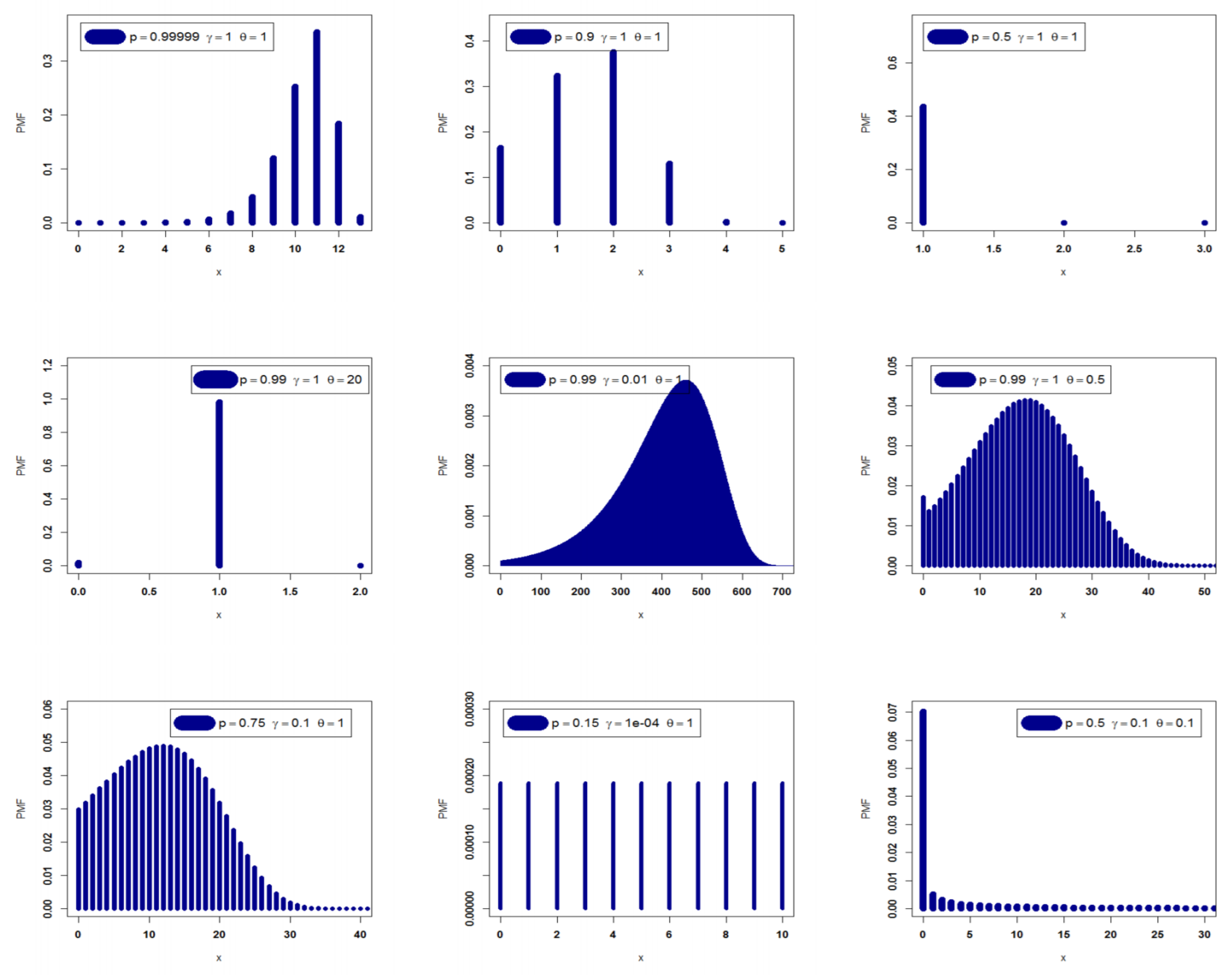
Funding

This research was funded by the Deputyship for Research and Innovation, Ministry of Education, Saudi Arabia, grant number QU-IF-2-5-3-25110.

Institutional Review Board Statement

Not applicable.

Informed Consent Statement

Not applicable.

Data Availability Statement

The four datasets are available in the paper.

Acknowledgments

The authors extend their appreciation to the Deputyship for Research & Innovation, Ministry of Education, Saudi Arabia for funding this research work through the project number (QU-IF-2-5-3-25110). The authors also thank Qassim University for technical support.

Conflicts of Interest

The authors declare no conflict of interest.

Abbreviations

RVRandom variable
PMFProbability mass function
CDFCumulative distribution function
EG-GExponential generalized G
DEG-GDiscrete exponential generalized G
exp-GExponential G
SFSurvival function
HRFHazard rate function
Disp-IxDispersion index
MLEsMaximum likelihood estimations
CVMECramér–von Mises estimation
OLSEOrdinary least squares estimation
BootstBootstrapping
KEKolmogorov estimation
WLSEWeighted least squares estimation
AD2LEAnderson–Darling method of left-tail second-order estimation
MSEMean square error
St.ErsStandard errors
MCMCMarkov chain Monte Carlo
l Log-likelihood
AICRAkaike information criterion
CAICRConsistent Akaike information criterion
BICBayesian information criterion
HQICHannan–Quinn information criterion
K–SKolmogorov–Smirnov
P.Vp-value
P–PProbability–probability
TTTTotal time in test
Q-QQuantile–quantile
FHRFFitted hazard rate function
FSFFitted survival function

References

  1. Nakagawa, T.; Osaki, S. The discrete Weibull distribution. IEEE Trans. Reliab. 1975, 24, 300–301. [Google Scholar] [CrossRef]
  2. Roy, D. Discrete Rayleigh distribution. IEEE Trans. Relib. 2004, 53, 255–260. [Google Scholar] [CrossRef]
  3. Jazi, A.M.; Lai, D.C.; Alamatsaz, H.M. Inverse Weibull distribution and estimation of its parameters. Stat. Methodol. 2010, 7, 121–132. [Google Scholar] [CrossRef]
  4. Gomez-Déniz, E. Another generalization of the geometric distribution. Test 2010, 19, 399–415. [Google Scholar] [CrossRef]
  5. Hesterberg, T. Bootstrap, Wiley Interdisciplinary Reviews: Computational Statistics. WIREs Comp. Stat. 2011, 3, 497–526. [Google Scholar] [CrossRef]
  6. Nekoukhou, V.; Bidram, H. The exponentiated discrete Weibull distribution. Stat. Oper. Res. Trans. 2015, 39, 127–146. [Google Scholar]
  7. Hussain, T.; Aslam, M.; Ahmad, M. A two-parameter discrete Lindley distribution. Rev. Colomb. Estad. 2016, 39, 45–61. [Google Scholar] [CrossRef]
  8. Para, B.A.; Jan, T.R. On discrete three-parameter Burr type XII and discrete Lomax distributions and their applications to model count data from medical science. Biom. Biostat. Int. J. 2016, 4, 1–15. [Google Scholar]
  9. El-Morshedy, M.; Eliwa, M.S.; Altun, E. Discrete Burr-Hatke distribution with properties, Estimation Methods and Regression Model. IEEE Access 2020, 8, 74359–74370. [Google Scholar] [CrossRef]
  10. El-Morshedy, M.; Eliwa, M.S.; Nagy, H. A new two-parameter exponentiated discrete Lindley distribution: Properties, estimation and applications. J. Appl. Stat. 2020, 47, 354–375. [Google Scholar] [CrossRef]
  11. Yousof, H.M.; Chesneau, C.; Hamedani, G.G.; Ibrahim, M. A new discrete distribution: Properties, characterizations, modeling real count data, Bayesian and non-Bayesian estimations. Statistica 2021, 81, 135–162. [Google Scholar]
  12. Chesneau, C.; Yousof, H.M.; Hamedani, G.; Ibrahim, M. A New One-parameter Discrete Distribution: The Discrete Inverse Burr Distribution: Characterizations, Properties Applications, Bayesian and Non-Bayesian Estimations. Stat. Optim. Inf. Comput. 2022, 10, 352–371. [Google Scholar] [CrossRef]
  13. Bourguignon, M.; Silva, R.B.; Cordeiro, G.M. The Weibull-G family of probability distributions. J. Data Sci. 2014, 12, 53–68. [Google Scholar] [CrossRef]
  14. Aboraya, M.M.; Yousof, H.; Hamedani, G.G.; Ibrahim, M. A new family of discrete distributions with mathematical properties, characterizations, Bayesian and non-Bayesian estimation methods. Mathematics 2020, 8, 1648. [Google Scholar] [CrossRef]
  15. Ibrahim, M.; Ali, M.M.; Yousof, H.M. The discrete analog of the Weibull G family: Properties, different applications, Bayesian and non-Bayesian estimation methods. Ann. Data Sci. 2021, 1–38. [Google Scholar] [CrossRef]
  16. Steutel, F.W.; van Harn, K. Infinite Divisibility of Probability Distributions on the Real Line; Marcel Dekker: New York, NY, USA, 2004. [Google Scholar]
  17. Eliwa, M.S.; Alhussain, Z.A.; El-Morshedy, M. Discrete Gompertz-G family of distributions for over-and under-dispersed data with properties, estimation, and applications. Mathematics 2020, 8, 358. [Google Scholar] [CrossRef]
  18. Yousof, H.M.; Majumder, M.; Jahanshahi, S.M.A.; Ali, M.M.; Hamedani, G.G. A new Weibull class of distributions: Theory, characterizations and applications. J. Stat. Res. Iran JSRI 2018, 15, 45–82. [Google Scholar] [CrossRef]
  19. Kemp, A.W. Classes of discrete lifetime distributions. Commun. Stat. Theor. Methods. 2004, 33, 3069–3093. [Google Scholar] [CrossRef]
  20. Poisson, S.D. Probabilité des Jugements en Matiére Criminelle et en Matiére Civile, Précédées des RéGles Génerales du Calcul des Probabilitiés; Bachelier: Paris, France, 1837; pp. 206–207. [Google Scholar]
  21. Aguilar, G.A.; Moala, F.A.; Cordeiro, G.M. Zero-Truncated Poisson Exponentiated Gamma Distribution: Application and Estimation Methods. J. Stat. Theory Pract. 2019, 13, 1–20. [Google Scholar] [CrossRef]
  22. Efron, B. The bootstrap and modern statistics. J. Am. Stat. Assoc. 2000, 95, 1293–1296. [Google Scholar] [CrossRef]
  23. Bodhisuwan, W.; Sangpoom, S. The discrete weighted Lindley distribution. In Proceedings of the International Conference on Mathematics, Statistics, and Their Applications, Banda Aceh, Indonesia, 4–6 October 2016. [Google Scholar]
  24. Lawless, J.F. Statistical Models and Methods for Lifetime Data; Wiley: New York, NY, USA, 2003. [Google Scholar]
  25. Chan, S.; Riley, P.R.; Price, K.L.; McElduff, F.; Winyard, P.J. Corticosteroid-induced kidney dysmorphogenesis is associated with deregulated expression of known cystogenic molecules, as well as Indian hedgehog. Am. J. Physiol.-Ren. Physiol. 2009, 298, 346–356. [Google Scholar] [CrossRef] [PubMed]
  26. Bebbington, M.; Lai, C.D.; Wellington, M.; Zitikis, R. The discrete additive Weibull distribution: A bathtub-shaped hazard for discontinuous failure data. Reliab. Eng. Syst. Saf. 2012, 106, 37–44. [Google Scholar] [CrossRef]
  27. Dougherty, E.R. Probability and Statistics for the Engineering, Computing and Physical Sciences; Prentice Hall: Englewood Cliffs, NJ, USA, 1992; pp. 149–152. ISBN 0-13-711995-X. [Google Scholar]
  28. Goual, H.; Yousof, H.M. Validation of Burr XII inverse Rayleigh model via a modified chi-squared goodness-of-fit test. J. Appl. Stat. 2020, 47, 393–423. [Google Scholar] [CrossRef] [PubMed]
  29. Yousof, H.M.; Ali, M.M.; Goual, H.; Ibrahim, M. A new reciprocal Rayleigh extension: Properties, copulas, different methods of estimation and modified right censored test for validation. Stat. Transit. New Ser. 2021, 23, 1–23. [Google Scholar] [CrossRef]
  30. Yadav, A.S.; Goual, H.; Alotaibi, R.M.; Ali, M.M.; Yousof, H.M. Validation of the Topp-Leone-Lomax model via a modified Nikulin-Rao-Robson goodness-of-fit test with different methods of estimation. Symmetry 2020, 12, 57. [Google Scholar] [CrossRef]
  31. Yadav, A.S.; Shukla, S.; Goual, H.; Saha, M.; Yousof, H.M. Validation of xgamma exponential model via Nikulin-Rao-Robson goodness-of- fit test under complete and censored sample with different methods of estimation. Stat. Optim. Inf. Comput. 2020, 10, 457–483. [Google Scholar] [CrossRef]
  32. Mansour, M.; Rasekhi, M.; Ibrahim, M.; Aidi, K.; Yousof, H.M.; Elrazik, E.A. A New Parametric Life Distribution with Modified Bagdonavičius–Nikulin Goodness-of-Fit Test for Censored Validation, Properties, Applications, and Different Estimation Methods. Entropy 2020, 22, 592. [Google Scholar] [CrossRef]
Figure 1. The PMF of the DEGW model.
Mathematics 10 03348 g001
Figure 2. The HRF of the DEGW model.
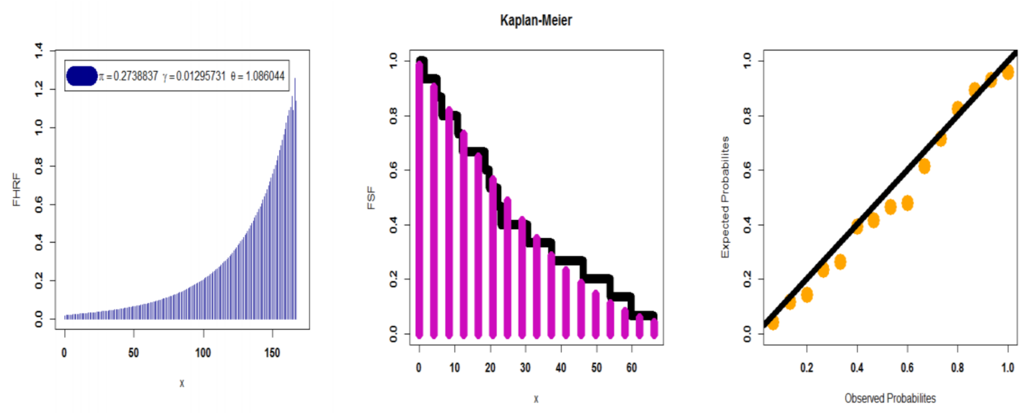
Mathematics 10 03348 g002
Figure 3. Kaplan–Meier plots based on dataset I.
Mathematics 10 03348 g003
Figure 4. Kaplan–Meier plots under dataset II.
Mathematics 10 03348 g004
Figure 5. Kaplan–Meier plots according to dataset III.
Mathematics 10 03348 g005
Figure 6. Kaplan–Meier plots for dataset IV.
Mathematics 10 03348 g006
Figure 7. Box, Q-Q, and TTT plots for dataset I.
Mathematics 10 03348 g007
Figure 8. The FHRF, ESF, and P–P plots for dataset I.
Mathematics 10 03348 g008
Figure 9. Boxplot, Q-Q plot, and TTT plot for dataset II.
Mathematics 10 03348 g009
Figure 10. The FHRF, ESF, and P–P plots for dataset II.
Mathematics 10 03348 g010
Figure 11. Boxplot, Q-Q plot, and TTT plot for dataset III.
Mathematics 10 03348 g011
Figure 12. The FPMF, FSF, FHRF, and FCDF plots for dataset III.
Mathematics 10 03348 g012
Figure 13. Boxplot, Q-Q plot, and TTT plot for dataset IV.
Mathematics 10 03348 g013
Figure 14. The FPMF, FSF, FHRF, and FCDF plots for dataset IV.
Mathematics 10 03348 g014
Table 1. Some new sub-models.
Baseline Model O z ; γ , ξ Sub Model
LL 1 + z γ 1 γ > 0 DEG LL
W e x p γ z θ 1 γ , θ > 0 DEGW
IW 1 e x p z θ γ 1 γ , θ > 0 DEGIW
E e x p γ z 1 γ > 0 DEGE
IE 1 e x p z 1 γ 1 γ , θ > 0 DEGIE
Lx 1 + z γ β 1 γ , β > 0 DEGLx
R e x p γ z 2 1 γ > 0 DEGR
IR 1 e x p z 2 γ 1 γ > 0 DEGR
Table 2. μ 1 , Z , μ 2 , Z , μ 3 , Z , and μ 4 , Z of the DEGW distribution.
W μ 1 , Z μ 2 , Z μ 3 , Z μ 4 , Z
(0.10, 1.0, 1.0)0.01913060.01913140.0191330.0191363
(0.50, 1.0, 1.0)0.31584390.33971450.3874670.4830028
(0.99, 1.0, 1.0)3.574481014.24669060.28199266.46120
(0.10, 0.5, 1.5)0.22530270.22684360.22992550.2360891
(0.50, 0.5, 1.5)0.75358850.98543511.45021002.3830030
(0.99, 0.5, 1.5)3.497186013.01448050.312590200.27770
(0.75, 0.1, 1.0)0.97134520.97364080.97823210.9874147
(0.75, 0.5, 1.0)0.82975440.82975440.82975440.8297544
(0.75, 1.0, 1.0)0.60998620.60998620.60998620.6099862
(0.75, 1.5, 1.0)0.36728410.36728410.36728410.3672841
(0.1, 0.1, 1.0)2.758169014.26941094.86910745.4975
(0.1, 0.1, 2.0)1.14198001.92594403.7041107.893829
(0.1, 0.1, 3.0)0.84441870.96340291.20137101.677308
(0.1, 0.1, 4.0)0.78503810.78526090.78570660.786598
(0.1, 0.1, 5.0)0.78492670.78492670.78492670.7849267
Table 3. Numerical results for E Z , V Z , S Z , and K Z of the DEGW distribution.
pγθE(Z)V(Z)S(Z)K(Z)Disp-Ix(Z)
0.999991110.435841.726577−1.0531855.1056380.1654468
0.9999 8.1341371.719510−1.0259134.9071830.2113943
0.999 5.8373831.673887−0.9292104.3310430.2867530
0.99 3.5744811.469777−0.6453383.2300670.4111861
0.75 0.7732450.5101060.4300222.2794380.6596955
0.5 0.3158440.2399571.0939882.8997620.7597332
0.1 0.0191310.0187657.02129750.303250.9809121
0.999991050.8023140.158607−1.5181943.3049120.1976864
0.9999 0.1105090.0982972.4846057.1732610.8894908
0.999 2.6895 × 10⁻¹⁰2.6895 × 10⁻¹⁰60976.45≈∞1
0.99 7.2967 × 10⁻⁹⁷7.2967 × 10⁻⁹⁷≈∞≈∞1
0.50.0012.512.74138018.070030−0.39365272.6058031.4182170
0.01 4.7714352.934613−0.38010662.625090.615038
0.1 1.59407800.5300682−0.29894352.8472070.3325235
0.25 0.93685910.2902798−0.05053573.3859810.3098437
0.5 0.63786160.2310265−0.57324781.3298230.3621891
0.65 0.53014510.2490913−0.12080011.0145930.4698549
0.75 0.46105160.24848300.15626861.024420.5389484
1.5 0.089517340.081503982.8756469.2693390.9104827
2.5 0.000430260.0004300948.178432322.1610.9995697
5 4.21 × 10⁻⁴⁵4.21 × 10⁻⁴⁵≈∞≈∞1
0.150.50.1471.22724739236251.070374085.929100572.2
0.50.58728311.4648223.01157415.061662.494234
10.33184280.30396231.4776744.4948780.9159829
50.29208740.20677240.91445951.8362360.7079126
200.29208740.20677240.91445951.8362360.7079126
1500.29208740.20677240.91445951.8362360.7079126
Table 4. Results of the MSEs where p = 0.1 ,   γ = 0.2 ,   θ = 0.9 .
n MLEOLSWLSCVMBayesianL-momKEBootstAD2LE
50 p 0 0.001110.001160.001780.001260.00069 *0.001400.001200.001550.00178
θ 0 0.00160 *0.020660.014520.017600.004300.002110.008850.002580.02066
γ 0 0.001130.000800.001120.000710.00042 *0.001440.000660.001300.00095
100 p 0 0.000580.000680.001060.000720.00052 *0.000820.000660.000960.00094
θ 0 0.00067 *0.008860.005080.008160.004150.000940.004560.002550.01008
γ 0 0.000580.000400.000630.000380.00036 *0.000830.000330.000760.00051
200 p 0 0.000260.000360.000650.000370.00022 *0.000370.000320.000320.00050
θ 0 0.00030 *0.004010.001860.003850.002540.000390.002210.000650.00493
γ 0 0.000260.000200.000370.000200.00014 *0.000370.000170.000280.00028
300 p 0 0.00019 *0.000250.000430.000250.000210.000240.000220.000230.00033
θ 0 0.00020 *0.002480.001180.002430.000780.000240.001540.000400.00315
γ 0 0.000200.000130.000250.000130.00009 *0.000240.000110.000170.00018
The value with “*” is the best estimation in its row for all estimation methods.
Table 5. Results of the MSEs where p = 0.5 ,   γ = 0.3 ,   θ = 0.6 .
n MLEOLSWLSCVMBayesianL-momKEBootstAD2LE
50 p 0 0.00336 *0.004030.004000.003910.005030.018250.003820.006790.00396
θ 0 0.004680.030630.030130.011050.006130.016390.00448 *0.00448 *0.01126
γ 0 0.00380 *0.011730.011550.010500.024080.024210.010260.013130.01065
100 p 0 0.00166 *0.001940.001930.001900.001980.012940.001730.002040.00192
θ 0 0.001780.006880.005240.005300.00099 *0.012240.001400.002120.00548
γ 0 0.00171 *0.005430.005370.005130.003920.014200.004380.002430.00520
200 p 0 0.00081 *0.001010.001020.001000.001620.009300.000900.001350.00101
θ 0 0.000830.002870.001750.002480.00039 *0.009190.000670.000830.00259
γ 0 0.00082 *0.002740.002750.002680.002970.009440.002210.002200.00271
300 p 0 0.00056 *0.000660.000670.000650.000680.006490.000570.001340.00065
θ 0 0.000570.001590.000800.001430.00035 *0.006490.000490.000650.00151
γ 0 0.00058 *0.001770.001800.001730.001480.006500.001370.002140.00175
The value with “*” is the best estimation in its row for all estimation methods.
Table 6. Results of the MSEs where p = 0.5 ,   γ = 0.3 ,   θ = 0.6 .
n MLEOLSWLSCVMBayesianL-momKEBootstAD2LE
50 p 0 0.00241 *0.003330.004980.003120.011590.003470.003080.003200.00480
θ 0 0.002420.002890.00189 *0.002500.004420.003390.002990.003270.00499
γ 0 0.002400.001190.002250.00105 *0.003160.003370.001060.003220.00202
100 p 0 0.001290.001750.003140.001700.003390.001810.001600.00111 *0.00265
θ 0 0.001300.001390.000740.001300.00042 *0.001800.001490.002180.00248
γ 0 0.001290.000590.001350.000560.00038 *0.001800.000530.001160.00108
200 p 0 0.00058 *0.000840.001950.000820.000630.000830.000790.000670.00132
θ 0 0.000590.000620.000320.000590.00019 *0.000820.000710.000560.00111
γ 0 0.000580.000270.000820.000260.00014 *0.000820.000260.000560.00053
300 p 0 0.000400.000490.001310.000490.00039 *0.000550.000480.000430.00078
θ 0 0.000400.000370.000180.000360.00014 *0.000550.000450.000430.00065
γ 0 0.000400.000160.000550.000160.00009 *0.000550.000150.000430.00031
The value with “*” is the best estimation in its row for all estimation methods.
Table 7. Results of the MSEs where p = 0.9 ,   γ = 0.9 ,   θ = 1.2 .
n MLEOLSWLSCVMBayesianL-momKEBootstAD2LE
50 p 0 0.000260.000280.000600.000260.00022 *0.000230.000300.002680.00046
θ 0 0.000410.006250.005780.005470.002710.00030 *0.004280.014360.00725
γ 0 0.000340.003420.010190.003180.002520.00026 *0.004630.016240.00783
100 p 0 0.00012 *0.000150.000350.000140.00012 *0.00012 *0.000160.000210.00023
θ 0 0.00012 *0.003370.002700.003080.002690.000140.002640.000530.00435
γ 0 0.00012 *0.001890.006530.001810.001610.000130.002460.000970.00375
200 p 0 0.00006 *0.000070.000200.000070.000100.00006 *0.000070.000060.00011
θ 0 0.00006 *0.001550.001070.001470.001050.00006 *0.001320.000190.00222
γ 0 0.00006 *0.000910.004120.000900.000960.00006 *0.001140.000180.00171
300 p 0 0.00004 *0.00004 *0.000140.00004 *0.000090.00004 *0.000050.000060.00007
θ 0 0.00004 *0.000840.000590.000820.001030.00004 *0.000840.000070.00138
γ 0 0.00004 *0.000550.003250.000550.000930.00004 *0.000720.000120.00110
The value with “*” is the best estimation in its row for all estimation methods.
Table 8. Comparing methods using dataset I.
MethodpγθK.SP.V
MLE0.84504412070.12488125820.68407501670.1630380.15266
OLS0.91153007230.45054030550.42491209610.169070.11468
WLS0.92730269870.44672007440.45721498910.200030.03659
CVM0.91832560580.45148886610.42885013930.175380.09231
* Bayesian0.83440242410.09876777650.72946842660.147120.22927
L-mom0.88836827380.13037784460.70194492190.168010.11884
KE0.01730978990.16199462740.00002039090.51000<0.0001
Bootst0.84654098510.12752350690.69484446780.213550.02092
AD2LE0.62156845270.13415561530.52979122710.220930.01518
The value with “*” is the best estimation in its row for all estimation methods.
Table 9. Comparing methods using dataset II.
MethodpγθK.SP.V
MLE0.27388366780.0129573141.08604411450.119980.98219
OLS0.19852571040.01681800050.98548234050.116030.98761
WLS0.23987468910.01802914360.99449317160.112290.99153
CVM0.13271547120.01036800761.04826192450.106790.99553
Bayesian0.30384624280.01992525870.99280280810.099370.99843
L-mom0.59012521290.05225615830.85825133400.124380.97446
KE0.00000331060.05863532190.00012654480.533310.00039
Bootst0.22445360220.01017426411.32469567800.318980.09447
* AD2LE0.00702309120.00249775581.24800675430.098850.99855
The value with “*” is the best estimation in its row for all estimation methods.
Table 10. Comparing methods using dataset III.
MethodpγθK.SP.V
MLE0.44594319050.73427721170.38005759390.356980.83653
OLS0.35722191760.6238149960.38614549420.338750.84419
WLS0.33512369320.59633143570.39775303340.381680.82627
CVM0.35597837270.6167014880.38504336140.284120.86757
Bayesian0.43343161300.67612787120.40339481130.617460.73438
L-mom0.65081957051.01298273190.36764231091.695470.42838
KE0.098589749960.50527932330.0933711548134.915<0.0001
Bootst0.45029071610.76588356570.38923165321.151920.56216
* AD2LE0.35605658790.61692321340.3834461730.283230.86796
The value with “*” is the best estimation in its row for all estimation methods.
Table 11. Comparing methods for dataset IV.
MethodpγθK.SP.V
MLE0.04219153210.14416607550.89868503592.073370.35463
OLS0.2074518880.26008609740.90269291402.061320.35677
WLS0.03280219270.12240198881.07414178972.573680.27614
CVM0.25601935470.29554076000.86423327272.000760.36774
Bayesian0.03881922230.12999532550.93350146732.216870.33007
* L-mom0.00001625860.04277207241.00549046841.340900.51148
KE0.02683904860.27324642667.22789×10⁻⁶8.69×10⁶<0.0001
Bootst0.03058122780.07878118521.0371758772117.888<0.0001
AD2LE0.40941464170.40168485410.87257948974.333180.11457
The value with “*” is the best estimation in its row for all estimation methods.
Table 12. The competitive models.
Discrete ModelAbbreviations
ExponentialDE
Inverse RayleighDIR
WeibullDW
Lindley-IIDLy-II
RayleighDR
Inverse WeibullDIW
Generalized exponential-IIDGE-II
Burr type XIIDBXII
LindleyDLi
Log-logisticDLL
LomaxDLx
PoissonPoisson
Exponentiated LindleyEDLy
ParetoDPa
Exponentiated WeibullEDW
Negative binomial (see Dougherty [27])NB
Table 13. The MLEs (and their corresponding St.Ers) for dataset I.
Modelpγθ
DEGW0.845040.124880.68408
(0.1316)(0.1337)(0.1787)
EDW0.989141.139340.78444
(0.1644)(3.2274)(3.0535)
DW0.981261.02342
(0.0114)(0.1322)
DIW0.018320.58244
(0.0131)(0.063)
DLy-II0.969340.0585
(0.00504)(0.0274)
EDLy0.972220.48020
(0.0053)(0.0873)
DLLc1.000100.43941
(0.3213)(0.0623)
DPa0.73922
(0.03212)
Table 14. The goodness-of-fit test statistics for comparing the competitive models for dataset I.
DEGWEDWDWDIWDLy-IIEDLyDLLcDPa
l233.47240.24241.65261.94240.67240.38294.99275.99
AICR472.93486.76487.25527.89485.23484.69593.84553.74
CAICR473.46487.29487.59528.18485.44484.88594.0553.84
K–S0.16300.19570.18720.25870.18680.19540.53540.3354
P.V0.15270.04570.06190.00360.064990.045<0.001<0.0013
Table 15. The MLEs (and their corresponding St.Ers) for dataset II.
Modelpγθ
DEGW0.273880.012961.08604
(0.83537)(0.0426)(0.48154)
DGE-II0.95611.4912
(0.0133)(0.535)
DIW2.3 × 10⁻⁴0.8752
(7.8 × 10⁻⁴)(0.164)
DLx0.0123104.506
(0.039)(84.409)
DBXII0.975313.367
(0.051)(27.785)
DR0.9992
(2.58 × 10⁻⁴)
DIR1.832 × 10⁻⁷
(0.055)
DPa0.7201
(0.061)
Table 16. The goodness-of-fit test statistics for comparing the competitive models for dataset II.
DEGWDEDGE-IIDRDIRDIWDLoDB-XII
l63.791165.00264.42366.39089.096468.70365.86475.724
AICR133.581134.02134.88134.83180.191141.413135.728155.45
CAICR135.763136.34135.81136.11180.501142.412136.728156.45
K–S0.119980.17770.12910.21610.69820.209230.205240.3889
P.V0.982190.67340.93730.4333<0.00010.48210.49120.0159
Table 17. The MLEs (and their corresponding St.Ers) for dataset III.
Modelpγθ
DEGW0.445940.734280.38006
(0.9079)(1.3168)(0.2637)
DW0.75030.43143
(0.084)(0.3402)
DIW0.58131.0492
(0.0483)(0.1463)
DLy-II0.58140.0011
(0.0455)(0.058)
DLx0.15051.8303
(0.0980)(0.9513)
DR0.90133
(0.0093)
DE0.5814
(0.0304)
DLi0.4363
(0.0263)
Poi1.3903
(0.1124)
Table 18. The goodness-of-fit test statistics for comparing the competitive models for dataset III.
ZOFDEGWDWDIWDRDExDLiDLy-IIDLxPoi
06564.16359.0163.9111.0046.0940.2546.0361.8927.42
11415.62619.8420.7026.8326.7829.8326.7721.0138.08
2109.18410.788.05029.5515.5618.3615.579.65026.47
366.0386.2604.23022.239.04010.359.0505.24012.26
444.1694.1902.6012.495.2505.5305.2703.1704.260
522.9552.0101.7505.4203.0502.8603.0602.0601.180
622.1271.9901.2601.8501.7701.4401.7801.4200.270
721.5451.3200.9500.5201.0300.7101.0401.0200.050
811.1280.9900.7400.1100.6000.3500.6000.7600.010
910.8270.8600.5900.0200.3500.1700.3500.5800.000
1010.6060.7600.4800.0000.2000.0800.2000.4600.000
1120.4451.9904.7400.0000.2800.0700.2802.7400.000
l 167.047170.14172.93277.78178.77189.1178.8170.48246.21
AICR 340.094344.28349.87557.56359.53380.2361.5344.96494.42
CAICR 340.321344.39349.98557.59359.57380.3361.6345.07494.46
χ V 2 0.356983.1256.463321.0722.8843.4822.893.316294.10
d.f 233444334
P.V 0.836530.3730.091<0.00010.0001<0.0001<0.00010.345<0.0001
Table 19. The MLEs (and their corresponding St.Ers) for dataset IV.
Modelpγθλ
DEGW0.042220.144170.89869
(0.12268)(0.13283)(0.1634)
DGW0.045032.5393242.15930.47933
(0.4293)(4.70345)(2.6988)(0.4655)
DIW0.345231.54132
(0.0433)(0.1564)
DBXII0.519332.35811
(0.0513)(0.3663)
NB0.870139.95623
(0.0364)(0.09623)
DIR0.31923
(0.0422)
DR0.86721
(0.01244)
DPa0.3299
(0.0344)
Poi1.48344
(0.0254)
Table 20. The goodness-of-fit test statistics for comparing the competitive models for dataset IV.
ZOFDEGWDIWDBXIIDIRDRNBDPaPoiDEGW
04346.55141.3743.8438.2815.9230.1264.4527.2346.551
13528.23841.8539.6151.9036.1738.8720.1540.3828.238
21718.31815.4215.6215.5134.5827.619.69029.9518.318
31111.5887.1707.2006.04021.0314.265.65014.8111.588
457.0303.9403.9102.9108.8905.9903.6805.4907.030
544.0522.4202.3701.6102.7002.1702.5801.6304.052
612.2021.6101.5600.9800.6000.7001.9000.4002.202
721.1201.1301.0900.6400.0900.2101.4600.0901.120
820.5305.0904.8002.1400.0200.06010.440.0200.530
l 200.956204.810204.293208.440235.23211.52220.63219.19200.956
AICR 407.912413.621412.587418.881472.45427.05443.24440.38407.912
CAICR 408.119413.723412.689418.915472.49427.14443.27440.41408.119
χ V 2 2.073375.5114.66414.27470.68820.36732.46238.4782.07337
d.f 233443442
P.V 340.321344.39349.98557.59359.57380.3361.6345.07494.46
Publisher’s Note: MDPI stays neutral with regard to jurisdictional claims in published maps and institutional affiliations.

