Predicting Perceptual Decision-Making Errors Using EEG and Machine Learning

Abstract

We trained an artificial neural network (ANN) to distinguish between correct and erroneous responses in the perceptual decision-making task using 32 EEG channels. The ANN input took the form of a 2D matrix where the vertical dimension reflected the number of EEG channels and the horizontal one—to the number of time samples. We focused on distinguishing the responses before their behavioural manifestation; therefore, we utilized EEG segments preceding the behavioural response. To deal with the 2D input data, ANN included a convolutional procedure transforming a 2D matrix into the 1D feature vector. We introduced three types of convolution, including 1D convolutions along the x- and y-axes and a 2D convolution along both axes. As a result, the $F1$-score for erroneous responses was above 88%, which confirmed the model’s ability to predict perceptual decision-making errors using EEG. Finally, we discussed the limitations of our approach and its potential use in the brain-computer interfaces to predict and prevent human errors in critical situations.

1. Introduction

Brain-computer interfaces (BCIs) have become a popular subject of scientific research in the fields of neurotechnology and neurorehabilitation [1]. In the most common paradigm, known as active BCI, the BCIs aim at decoding brain activity into the control commands for the external devices. Using active BCI, the operator thought to generate the mental commands at any time they want without external assistance. For instance, a person with paraplegia may make the wheelchair move in different directions [2]. Another paradigm, reactive BCI, complements an active BCI with external stimulation, helping the operator to generate mental commands [3]. In a popular reactive BCI called P300 speller, a subject looks at a display where characters are flashing and selects one character by attending to it [4]. In the wheelchair control, this display may contain flashing symbols reflecting different directions of movement. Finally, a passive BCI paradigm implies monitoring brain state and signalling when it deviates from the normal [5]. This idea stands behind the closed-loop antiepileptic device, a brightest example of the passive BCIs [6,7].

Passive BCIs may give rise to assistive technologies (AT) that monitor brain activity in resource-demanding tasks [8,9]. Analysing EEG signals in on-line mode, AT may detect fatigue, loss of attention, and other states in which the performance declines. Being built in the car, AT will advise to have a rest after many hours of driving. In the aircraft, it could detect the pilot’s fatigue and inform the co-pilot. Similarly, flight operations officers or power plant operators may finish their shift earlier once AT have found the biomarkers of fatigue in their EEG [10]. However, this concept faces challenges when transiting from the lab to real-life applications. First, AT decode brain states, which reflect the increasing probability of performance decline but do not guarantee its appearance. When diagnosing mental fatigue, we expect a high risk of errors. At the same time, the operator makes errors when the signs of fatigue are absent on EEG signals. Second, the brain state changes in a manner far from monotonous. Thus, together with an expected drop of attention with the time on task, it fluctuates within short timescales so that AT predicts the performance to decline very often. To overcome these challenges, AT should predict the error itself rather than detect a state when its probability is high. It will enable the target assistance only when it is necessary.

In this manuscript, we made the first step towards the perceptual errors’ prediction in the brain-computer interfaces—we proposed a machine learning model that predicts errors from the short EEG segments on a single-trial basis. To collect behavioural data and brain activity signals, we used a perceptual decision-making task, an experimental paradigm that requires participants to perceive visual stimuli on the screen and respond to them using joystick. In this paradigm, the participants were subjected to perceive 400 stimuli in a row with a brief interval. It simulated the real-life situation that implies the decision making under stress and pressure. To increase the probability of errors, we used ambiguous stimuli and decreases the stimulus exhibition time. As the result, the subjects make errors in 13% of responses.

The literature suggests that the neural activity registered before the stimulus onset carries biomarkers of the observer’s state, affecting the decision on an ongoing stimulus [11]. Therefore, we expect that ANN will learn to distinguish between the errors and correct responses using the pre-stimulus EEG segments as the input. Recent studies on the perceptual decision-making report that this process involves two components: sensory processing and decision-making. The sensory processing dominates during the early time window (about 300 ms, $30\%$ of the whole decision time) [12,13]. There is a view that the brain matches sensory information with an internal template, even in the early sensory-processing stages. Therefore, we expect that neural activity registered during 300 ms post-stimulus onset also influences the final decision on the stimuli and may also serve as ANN input.

We merged the data of all subjects and trained artificial neural network (ANN) to classify (correct vs. incorrect) responses from the EEG fragments. The following results were obtained:

• We demonstrated that ANN can predict errors in the perceptual-decision-making task using EEG signals recorded before the behavioural response with the accuracy above $85\%$.
• To form the input data for ANN, we averaged neural activity over time and over the sensors. In both cases, the classification accuracy remained above $85\%$ manifesting that both dimensions contain valuable discriminating features.
• Using prestimulus and post-simulus EEG segments as input data resulted in the classification accuracy above $85\%$. The prestimulus EEG reflect human state while post-stimulus EEG reflect the sensory processing mechanisms. Thus, we concluded that these processes affect the final decision.

Finally, we discussed the future development of error decision-making prediction in assistive BCIs.

This manuscript has the following structure. Materials and Methods section contains description of the experiment including the recruitment, EEG recording and the type of perceptual decision-making task, es well as the data analysis pipeline including preprocessing, feature selection, machine-learning model, its hyperparameters and cross-validation procedure. Results section presents the outcomes of the ML application in terms of accuracy, F1-score, sensitivity and specificity. This section also reports the effect of ML hyperparameters and the class imbalance on the classification scores. Finally, Discussion section summarizes the results, pays attention to the limitation of our paradigm, and its potential use in the brain-computer interfaces to predict and prevent human errors in critical situations.

2. Materials and Methods

In this section, we described experimental paradigm and data analysis framework. The description of experimental paradigm includes recruitment process, visual stimuli (Necker cubes), design of experiment, and behavioural estimates resulted in separating data in two classes. The description of data analysis framework includes preprocessing, feature selection, machine learning model, and cross-validation.

2.1. Participants

Thirty naive healthy subjects (16 females) aged 18–33 years (M = $22.1$, SD = $2.68$) with no previous psychiatric or neurological history participated in the experiments. Individual neuroimaging studies typically involve 12–20 participants [14]. At the same time, 30 is the smallest sample size that allows using central limit theorem [15]. All the subjects have normal or corrected-to-normal visual acuity. All of them provided written informed consent in advance. The study was approved by the local ethics committee of the Lobachevsky State University of Nizhny Novgorod (ethical approval number 2, dated 19 March 2021) and was following the Declaration of Helsinki, except for registration in a database.

2.2. EEG Recording

We registered electroencephalograms (EEG) using a 48-channel NVX-52 amplifier (MKS, Zelenograd, Russia). EEG signals were recorded from 32 standard Ag/AgCl electrodes (Fp1, Fp2, F3, Fz, F4, Fc1, Fc2, F7, Ft9, Fc5, F8, Fc6, Fc10, T7, Tp9, T8, C3, Cz, C4, Cp5, Cp1, Cp2, Cp6, Cp10, P7, P3, Pz, P4, P8, O1, Oz, O2), placed according to the international 10–10 system. The earlobe electrodes were used as a reference. The ground electrode was placed on the forehead. Impedance was kept below 10 K$\Omega$. EEG was digitized with a sampling rate of 1000 Hz.

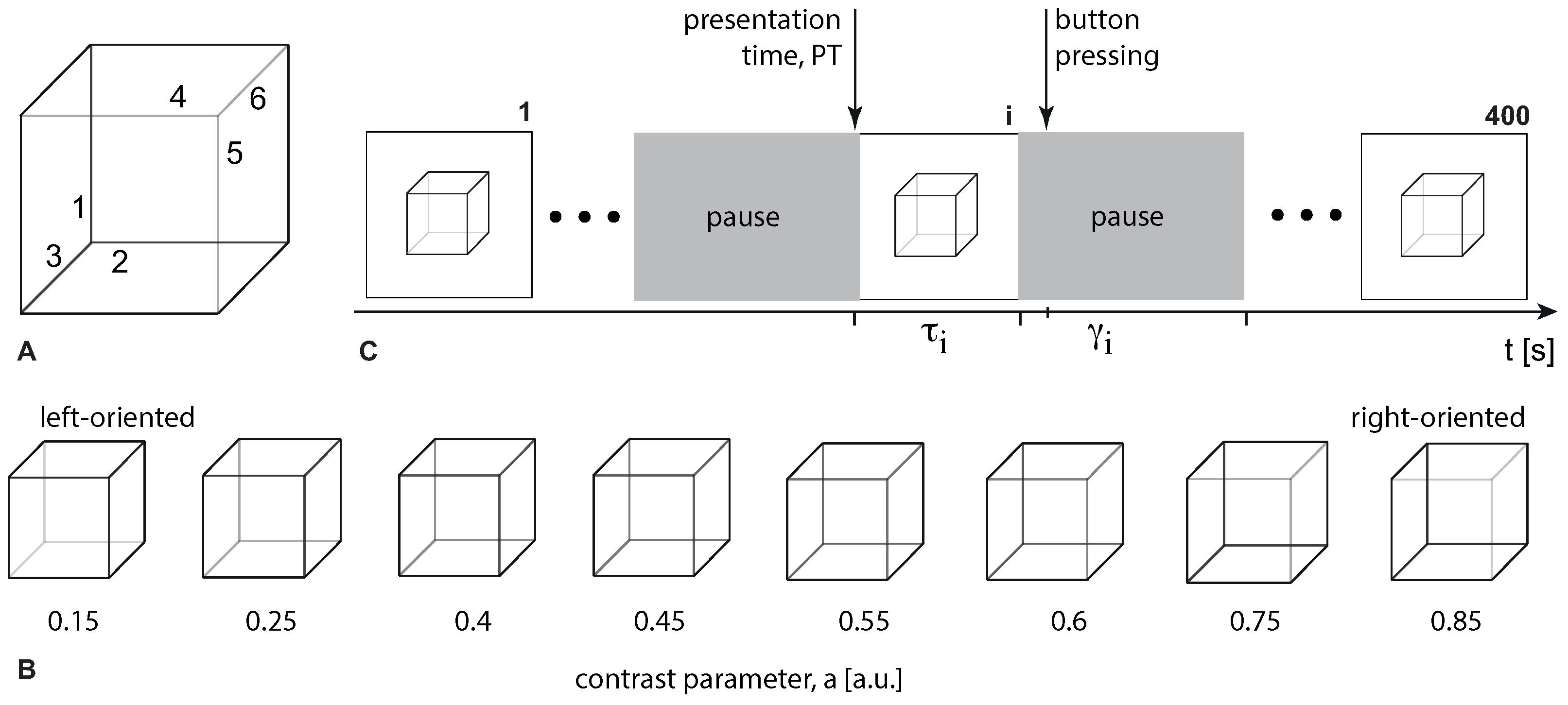
2.3. Visual Stimulus

We used Necker cubes as visual stimuli. Figure 1 illustrates the set of visual stimuli—Necker cube images with the different contrast of the inner edges [16]. For each cube, we introduced parameter $a=0.15,0.25,0.4,0.45,0.55,0.6,0.75,0.85$ defining the inner edges contrast. It reflected the intensity of three lower-left lines, while $1-a$ corresponded to the intensity of three upper-right lines. The parameter a can be defined as $a=1-y/255$, where y is the brightness level of three lower-left lines using the 8-bit gray-scale palette. The value of y varies from 0 (black) to 255 (white).

2.4. Experiment

During the experiment, participants were comfortably seated in a reclining chair. With both hands, they held a two-button input device connected to the amplifier. Participants were instructed to stay relaxed with open eyes during the entire experiment unless performing a task. At the beginning and at the end of the experiment, we recorded resting-state EEG activity for 3 min. The Necker cube images of 25.6 cm were displayed on a 27-inch LCD screen (with the 1920 × 1080 pixels resolution; 60 Hz refresh rate) located at a distance of 2 meters from the participant. Each cube appeared on the screen for a short time interval, randomly chosen from the range 1–1.5 s. Between the stimuli, we demonstrated an abstract image for 3–5 s. The timing of Necker cubes presentations and the EEG streams were synchronized using a photodiode connected to the amplifier. During experimental sessions, the cubes with predefined ambiguity (see all images in Figure 1) were randomly demonstrated 400 times, each cube with a particular ambiguity was presented about 50 times. Participants were instructed to press either the left or right key when recognizing the left or the right stimulus orientation. The experiment lasted around 45 min.

2.5. Behavioural Estimates and Definition of Classes

For each participant, we calculated error rate ER as the percentage of erroneous responses. The correctness of each response was evaluated by comparing the actual stimulus orientation with the subject’s response. The actual orientation of the Necker cube was defined by the contrast of the inner edges. Thus, a = 0.15, 0.25, 0.4, 0.45 defined the left-oriented cubes, while a = 0.55, 0.6, 0.75, 0.85 stood for the right-oriented ones. To define the correctness, we checked whether the subject pressed the left button for a = 0.15, 0.25, 0.4, 0.45, or the right button for a = 0.55, 0.6, 0.75, 0.85. Otherwise, their response was incorrect. ER varied from $0.54\%$ to $83\%$ in the group of participants (M = $13\%$, SD = $14\%$). We excluded four participants whose ER was lower than $2.1\%$ (5 percentile) and higher than $28.6\%$ (95 percentile) from the consideration.

We tested how the ER depends on the type of stimulus using repeated measures ANOVA. Stimulus ambiguity (High vs. Low) and stimulus orientation (Left vs. Right) were taken as within-subject factors. As a result, we found a significant main effect of ambiguity: F(1,25) = 65.13, p < 0.001, The main effect of orientation was insignificant F(1,25) = 0.88, p = 0.375. Finally, we reported an insignificant interaction effect of Ambiguity and Orientation: F(1,25) = 0.02, p = 0.888. The post-hoc t-test revealed, the ER for High ambiguity (M = $18.2\%$, SE = $2.02$) exceeded ER for Low ambiguity (M = $3.3\%$, SE = $0.53$): $p<0.001$, Bonferroni correction.

2.6. Data Analysis

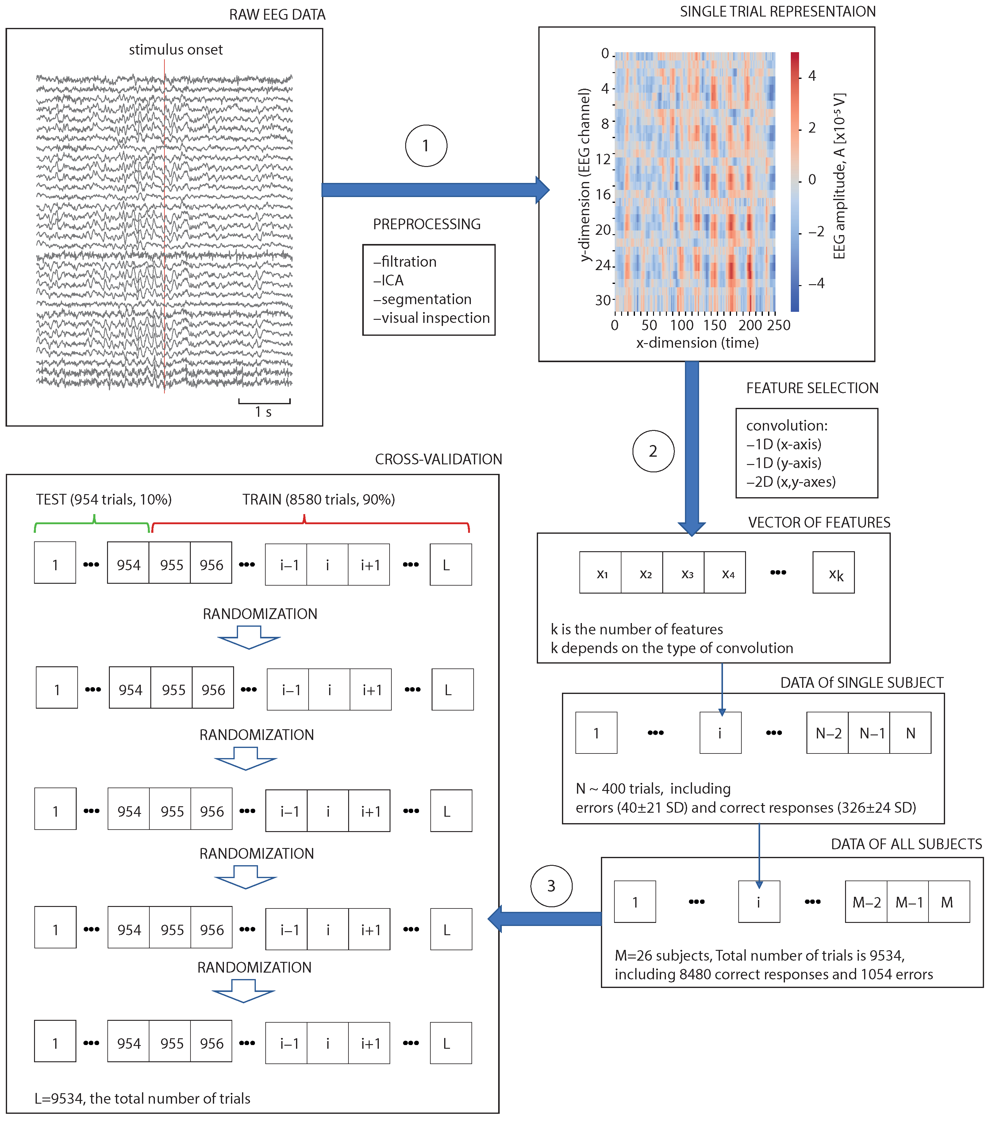
The overall data analysis framework includes three main steps (Figure 2): preprocessing (1), feature selection (2), and cross-validation (3). In the preprocessing block, we filtered raw EEG, removed ICAs with artefacts, segmented signals into the trials and removed bad segments. In the convolution block, we performed dimension reduction by averaging EEG signals over time and/or over the sensors. In the cross-validation block, we combined data of all subjects and divided trials into the test (10%) and train ($90\%$) sets. This procedure was repeated five times followed by randomising the trials. All scores were averaged over the five rounds of cross-validation.

Preprocessing. We filtered EEG signals with a fourth-order Butterworth $(1-100)$-Hz bandpass filter and a 50-Hz notch filter. In addition, we performed an independent component analysis (ICA) to remove eye blinking and heartbeat artifacts. These pre-processing procedures were carried out in Matlab using EEGLAB software. We then segmented EEG signals into 4-s trials associated with a single presentation of the Necker cube, including a 2-s interval before and 2-s interval after the moment of the stimulus demonstration. After the visual inspection, we excluded some trials due to the remaining large-amplitude artifacts. To exclude trials containing large amplitude artifacts, we used the z-value threshold $z<1$. The rejection procedure was performed using the FieldTrip toolbox in Matlab. After the rejection, we had $40\pm 21$ SD erroneous and $326\pm 24$ SD correct trials per subject.

Feature selection. We considered each trial as a $(32\times 375)$ matrix containing values of EEG amplitude at each channel at a 1.5 s interval (time of interest, TOI1), including 1 s prestimulus (TOI3) and 0.5 post-stimulus (TOI2) segments. This matrix served as an input for the convolutional procedure. We supposed that TOI3 stored information about the participant’s condition, including their fatigue and attention. These processes affect neuronal activity regardless of the task, but may produce a strong impact on the decision accuracy. The neural activity at TOI2 reflected sensory processing. In line with the Ref. [12] we hypothesized that sensory processing prevails during the earlier temporal window, while decision-making lasts for a prolonged time and dominates before the behavioural response. At the same time, there is a view that perceptual decision-making is an iterative process, so even in the early stages, the brain matches sensory evidence with the internal templates to make the decision. Thus, neural activity at TOI2 may also affect the decision accuracy. Here, we tested whether we could classify the correct and erroneous responses using EEG data at TOI2 and TOI3. We used three different input matrices containing values of EEG amplitude at 32 channels:

• for TOI1—the $(32\times 375)$ matrix;
• for TOI3—the $(32\times 250)$ matrix;
• for TOI2—the $(32\times 125)$ matrix.

Convolution. Each input ($m\times n$) matrix underwent a convolutional procedure that reduced their height and width. We implemented different types of convolution as follows:

• 1D convolution (y-axis)—convolution only slides along the channel dimension (y-direction) where the time dimension (x-direction) is fixed. In this case, we averaged EEG amplitude across all channels at every moment. As a result, the ($m\times n$)-matrix was reduced to the m-dimensional feature vector, where m reflected the length of time interval (TOI1, TOI2, or TOI3);
• 1D convolution (x-axis)—convolution only slides along the time dimension (x-direction) where the time dimension (y-direction) is fixed. In this case, we averaged EEG amplitude over time for all channels. As a result, the ($m\times n$)-matrix was reduced to the m-dimensional feature vector, where m = 32 reflected the number of EEG channels;
• 2D convolution (x,y-axes)—convolution slides along both channel and time dimensions. First, averaging EEG amplitude across all channels leads to the m-dimensional feature vector, where m is the length of interval. Defining the length of resulting feature vector k, we segmented the time interval into k equal pieces. Finally, averaging EEG amplitude in each segment forms the k-dimensional feature vector. In this approach, k is a hyperparameter.

Cross-validation. After the convolutional procedure, we loaded the feature vector to the artificial neural network (ANN) implemented using the TensorFlow library in Python. We trained ANN to distinguish between the correct and erroneous responses and evaluated its efficiency using cross-validation. Merging the data of all the participants, we formed a dataset of 9534 trials, 8480—correct and 1054—erroneous. Each round of cross-validation involved partitioning a dataset into two subsets, performing ANN training on the training subset (8580 trials, $90\%$), and validating on the testing subset (954 trials, $10\%$).

In each round, we estimated the model’s performance using categorical accuracy, sensitivity and specificity. To reduce variability, we performed five rounds of cross-validation using different partitions and averaged metrics over the rounds.

Hyperparameters. We tested how the ANN’s performance changed depending on the variations of the basic hyperparameters.

Optimizer—an algorithm used to change the attributes of the neural network such as weights and learning rate in order to reduce the losses. We used the following optimizers: Stochastic gradient descent; Root-mean square propagation; Adam; Adaptive Gradients (Adagrad); Adam optimizer with the infinity norm (Adamax); Adam optimizer with Nesterov momentum (Nadam).

Initializer—a technique that defines the way to set the initial random weights of ANN layers. Here, we used the following initializers: Xavier normal initializer, Xavier uniform initializer; He normal initializer; He uniforms initializer; Lecun Normal initializer; Lecun Uniform initializer; Orthogonal initializer; Random normal initializer; RandomUniform initializer; Glorot normal initializer; Truncated normal distribution; Variance Scaling.

The activation function defines how the neuron transforms the weighted sum of the input into an output. Here, we set the following activation function to the neurons in the intermediate layer: relu; sigmoid; softmax; softplus; softsign; tanh; selu; elu; exp.

Learning rate—a hyperparameter that controls how much to change the ANN model in response to the estimated error each time the model weights are updated. A small learning rate may result in a long training process, whereas a large learning rate may result in learning a sub-optimal set of weights too fast or an unstable training process.

Batch size defines the number of samples that will be propagated through the network. If the batch size is equal to 100, the algorithm takes the first 100 samples from the training dataset and trains the network. Next, it takes the second 100 samples (from 101st to 200th) and trains the network again. We can keep doing this procedure until we have propagated all samples through the network.

The number of epochs defines the number of times that the learning algorithm will work through the entire training dataset. One epoch means that each sample in the training dataset has had an opportunity to update the internal model parameters. When the number of epochs is large, the ANN learns patterns that are specific to sample data to a great extent. As a result, ANN gives high accuracy on the training set but fails to achieve good accuracy on the test set.

Handling imbalanced dataset. First, we used additional metrics to evaluate the model’s performance. Thus, we calculated precision and recall for each class. Then, we calculated $F1$-score of a class as the harmonic mean of precision and recall $(2\times precision\times recall/(precision+recall\left)\right)$. If both $precision$ and $recall$ were high resulting in the high $F1$, we concluded that this class was perfectly handled by the model. Using the $F1$ score for errors, we evaluated whether undersampling the dataset could improve the model performance. Undersampling is a procedure that implies sampling from the majority class (the correct responses) to keep only a part of these points. There are different rules for undersampling, but we utilized the random undersampling. Thus, we randomly removed the part of data from the class of correct responses so that the proportion class1:class2 varied from 1:8 to 1:1.

Finally, there is a view that if two classes are separated enough (far apart from each other in the feature space), the imbalance between them may be compensated. One way to increase separability is enriching the dataset with additional features. To test how the separability influences the model performance, we used 2-D convolution to compress the input matrix to the 1-D vector of k-features. First, we evaluated how the Euclidian distance between classes changed with growing k. Then, we analyzed whether the $F1$ score varied with changing k.

3. Results

We started with the ANN containing a single intermediate layer and the following hyperparameters: initializer = RandomUniform, intermediate layer activation function = softmax, Adam optimizer, learning rate = 1, batch size = 200, number of epochs = 10. This configuration provided $88\%$ accuracy for the 1D convolution across the x-axis and $88.9\%$—for the 1D convolution across the y-axis. In the first case, the convolution formed a vector $\mathbf{A}=(A_1\cdots A_m)$ where $m=32$ is the number of EEG channels. In the second case, we obtained a vector $\mathbf{A}=(A_1\cdots A_m)$ where m depended on the time interval, taking the value of 375 (for TOI1), 125 (for TOI2), and 250 (for TOI3). For the 2D convolution, we tested how the ANN accuracy depended on the vector size k obtained after the convolution. As a result, the optimal value, $k=47$, resulted in $91.6\%$ accuracy.

When running the ANN with a different number of intermediate layers, we found that accuracy fluctuated from $88.1\%$ (for 4 layers) to $89.9\%$ (for 1 layer). There was neither monotonic growth nor a decrease of the accuracy with the number of layers. Thus, we proceeded with a single intermediate layer to decrease computational costs.

Then, we considered different weight initialization techniques and found the highest accuracy of $92.6\%$ for the orthogonal initialization generating an orthogonal matrix. For the other initialization techniques, accuracy varied from $87.7\%$ (for the Glorot normal initializer) to $90.4\%$ (for the He initializer).

Considering different activation functions, we found that $rely$ provided the highest accuracy of $92.6\%$, while $softplus$ resulted in the lowest accuracy of $88.8\%$. We used $rely$ only for the neurons in the transient layer. On the output layer, we proceeded with $sigmoid$ function, a common option for the binary classification task.

We utilized different optimizers to adjust the ANN attributes and achieved the highest accuracy of $91\%$ for Adagrad optimizer and the lowest accuracy of $88\%$ for the Root Mean Squared Propagation.

When changing the learning rate (LR) from ${10}^{-5}$ to ${10}^{-3}$, we observed weak nonsystematic changes in the accuracy in the range from $88\%$ (for LR = ${10}^{-5}$ ) to $91\%$ (for LR = ${10}^{-4}$).

When changing the batch size from 300 to 4000, we also observed weak nonsystematic changes in the accuracy in the range from $87.8\%$ (for batch size = 200) to $89.5\%$ (for batch size = 500).

To find an optimal number of epochs, we varied this parameter from 1 to 100. For each value, we trained ANN with the five different batch sizes and averaged the resulting accuracies. For the number of epochs = 1, ANN gave an accuracy of $89.7\%$. the further enlargement of the number of epochs only slightly enhanced the accuracy to $89.9\%$.

Finally, we run the ANN with the optimal hyperparameters (initilizer = $Orthogonal$, activation function = $relu$, optimizer = $Adagrad$, learning rate = $0.0001$, batch size = 500, epochs = 1) to classify the responses (correct vs. incorrect) using the different types of convolution and the different fragments of EEG signals. As a result, classification accuracy varied in a narrow range of 88.4–89% achieving $89\%$ for TOIs 1,3 and the 1D convolution along the y-axis, and $88.4\%$ for TOI1 and 1D convolution along the x-axis (

Table 1. The classification accuracy depending on the convolution type and the EEG segment.

Convolution Type	$\mathit{TOI}1$	$\mathit{TOI}2$	$\mathit{TOI}3$
1D convolution (x-axis)	$88.4\%\pm 0.3\%$SD	$88.6\%\pm 0.3\%$SD	$88.5\%\pm 0.2\%$SD
1D convolution (y-axis)	$89\%\pm 0.07\%$SD	$88.8\%\pm 0.2\%$SD	$89\%\pm 0.1\%$SD
2D convolution (x,y-axes)	$88.8\%\pm 0.2\%$SD	$88.5\%\pm 0.2\%$SD	$88.9\%\pm 0.1\%$SD

).

Considering the $F1$-scores for each class, we found that it varied from 87.8% to 88.1% for the erroneous responses (

Table 2. The $F1$-score for erroneous responses depending on the convolution type and the EEG segment.

Convolution Type	$\mathit{TOI}1$	$\mathit{TOI}2$	$\mathit{TOI}3$
1D convolution (x-axis)	$87.9\%\pm 0.1\%$ SD	$87.9\%\pm 0.2\%$ SD	$88\%\pm 0.2\%$ SD
1D convolution (y-axis)	$87.8\%\pm 0.1\%$SD	$87.8\%\pm 0.1\%$SD	$87.9\%\pm 0.05\%$SD
2D convolution (x,y-axes)	$88.1\%\pm 0.3\%$SD	$87.9\%\pm 0.1\%$SD	$87.9\%\pm 0.2\%$SD

) and from 88% to 88.2% for the correct responses (

Table 3. The $F1$-score for correct responses depending on the convolution type and the EEG segment.

Convolution Type	$\mathit{TOI}1$	$\mathit{TOI}2$	$\mathit{TOI}3$
1D convolution (x-axis)	$88.2\%\pm 0.1\%$SD	$88.1\%\pm 0.2\%$SD	$88\%\pm 0.2\%$SD
1D convolution (y-axis)	$88.1\%\pm 0.1\%$SD	$88.1\%\pm 0.1\%$SD	$88.2\%\pm 0.05\%$SD
2D convolution (x,y-axes)	$88.1\%\pm 0.1\%$SD	$88.1\%\pm 0.2\%$SD	$88.2\%\pm 0.1\%$SD

).

Considering the sensitivity, we found that it varied from 86.8% to 87.6% (

Table 4. The sensitivity depending on the convolution type and the EEG segment.

Convolution Type	$\mathit{TOI}1$	$\mathit{TOI}2$	$\mathit{TOI}3$
1D convolution (x-axis)	$87.1\%\pm 0.1\%$SD	$87.1\%\pm 0.1\%$SD	$87.6\%\pm 0.4\%$SD
1D convolution (y-axis)	$86.8\%\pm 0.1\%$SD	$86.8\%\pm 0.1\%$SD	$86.8\%\pm 0.04\%$SD
2D convolution (x,y-axes)	$86.9\%\pm 0.1\%$SD	$86.9\%\pm 0.1\%$SD	$87.1\%\pm 0.3\%$SD

). The specificity varied from 88.9% to 89.2% (

Table 5. The specificity depending on the convolution type and the EEG segment.

Convolution Type	$\mathit{TOI}1$	$\mathit{TOI}2$	$\mathit{TOI}3$
1D convolution (x-axis)	$89\%\pm 0.2\%$SD	$88.9\%\pm 0.3\%$SD	$88.7\%\pm 0.3\%$SD
1D convolution (y-axis)	$89.1\%\pm 0.09\%$SD	$89.1\%\pm 0.1\%$SD	$89.2\%\pm 0.05\%$SD
2D convolution (x,y-axes)	$89.1\%\pm 0.1\%$SD	$89.1\%\pm 0.06\%$SD	$89.1\%\pm 0.2\%$SD

).

Addressing the imbalance problem, we randomly removed the part of data from the class of correct responses so that the proportion (erroneous:correct) varied from 1:1 to 1:8. We found that $F1$-score for the erroneous responses decreased for undersampled data. Thus, $F1$-score was equal to $40\%$ for 1:1 ratio, while for 1:8 $F1$ increased to $83\%$.

To study the class separability in the feature space, we calculated the Euclidean distance between their centroids. We analysed how the distance between classes depends on the number of features, k, obtained after the 2D convolution. As expected, the distance grows with increasing k. At the same time, the classification score does not exhibit systematic changes with the growing distance.

4. Discussion

We trained ANN to distinguish between the correct and erroneous responses to the visual stimulus using 32 EEG signals recorded from the different parts of the scalp. The ANN input took the form of a 2D matrix where the vertical dimension (y-axis) reflected the number of EEG channels, and the horizontal (x-axis) dimension reflected the considered time interval.

We focused on distinguishing the responses before their behavioural manifestation; therefore, we utilized EEG segments preceding the behavioural response. They included a 1-s trace preceding and a 0.5-s trace following the stimulus onset. We observed the behavioural responses 1 second after the stimulus onset.

To deal with the 2D input data, ANN included a convolutional procedure, transforming a 2D matrix into the 1D feature vector. We introduced three types of convolution, including 1D convolutions along the x- and y-axes and a 2D convolution along both axes.

We studied how the ANN’s output changed depending on variations of the ANN hyperparameters. Summarising the results, we concluded that ANN gives about 90% accuracy. Manipulations with the input data, including the length of EEG trace and the convolution type, lead to slight deviations in the accuracy. Similarly, accuracy changes from 88% to 90% when varying the ANN hyperparameters. These results confirm that ANN may predict perceptual errors using EEG signals. Finally, due to the small number of perceptual errors, we addressed the class imbalance problem by undersampling the majority class of the correct responses. We observed that undersampling reduces the classification score. Thus, we concluded that the rare nature of errors might be their distinguishing feature required for the classification.

Our study has a potential limitation arising from the specific features of the human data. First, cross-validation only yields meaningful results if the testing and training sets belong to the same population. To obey this criterion, we merge data of all subjects and randomly divide all trials into the training and testing sets. Thus, both sets may include trials of one subject ensuring their drawing from the same distribution. At the same time, EEG data may vary between participants and even between the different trials recorded in the different phases of the experiment. These issues, known as cross-subject and cross-trials problems [17] could be addressed by subspace learning, a type of the transfer learning [18]. This approach consists in extracting a subset containing the common features of the trials in one class and excluding varying components [19].

As we showed in Ref. [20], the feature subset may include features obtained from the statistical contrast between classes using the within-subject design. For the current task, it means averaging EEG features across the correct and erroneous trials for each subject and contrasting the obtained mean values using the paired-samples statistics. Our ongoing study will use the statistical contrast of the EEG spectral power (SP) between the correct and erroneous responses to find EEG channels and frequencies where SP differs between the correct and erroneous responses regardless of between-subject variability.

A bulk of literature describes employing a similar predictive analysis in BCIs to control motor activity and decision making. In 2011, Bai and colleagues used EEG signals to predict natural human movement before it occurs in real time [21]. Measuring muscle activity, they captured the start of movement and reported its prediction for 0.6 s. To extract features from EEG signals, the authors used Surface Laplacian derivation and the Welch-based power spectral density estimation. Loading the extracted features to the multivariate linear classifier, they correctly predicted 40% of total moves. A year later, Maeder et al. utilized the pre-stimulus EEG signals in the motor-imagery BCI [22]. They addressed how the pre-stimulus sensorimotor rhythms (SMR) amplitude influences the successive task execution quality and the classification performance. Using Common Spatial Patterns preprocessing and Linear Discriminant Analysis, they reported that higher SMR amplitude predicts better classification performance. In their work, Meinel et al. also used pre-trial EEG to predict performance in the sequential isometric force control task, a paradigm for hand motor rehabilitation after stroke [23]. They assessed performance using the clinically relevant metrics, including reaction time, smoothness, and precision of the produced force trajectory. To predict them, they trained the regression model, Source Power Comodulation where predictors were selected through the feature extraction procedure. As a result, their model explained up to 36% of the performance fluctuations in the motor rehabilitation scenario. In 2015, Lin et al. combined EEG signal analysis with behavioural modeling to predict Human Errors in Numerical Typing [24]. Using Linear Discriminant Analysis, they reported a reasonable classification performance of 0.63 in terms of AUC. A recent work by Dehais and colleagues describes the passive BCI prototype, which predicts attentional error before it happens in flight conditions [25]. They instructed pilots to fly a challenging flight scenario while responding to auditory alarms by button press. The behavioural results disclosed that the pilots missed 36% of the auditory alarms. The authors used EEG signals recorded for 3 s before the alarm to train different classifiers including Supervised Dictionary techniques, Nearest Neighbour, and Linear Discriminant Analysis. In the best case, they reported a classification performance of up to 70%. Finally, Fernandez-Vargas et al. proposed another prospective application of the pre-stimulus activity in BCIs [26]. They found the subject- and task-independent neural correlates of decision confidence and proposed an algorithm to estimate decision confidence on a trial-by-trial basis. The authors further suggested that confidence in perceptual decision-making tasks could be reconstructed from neural signals even when using transfer learning approaches.

According to this review, using a predictive paradigm in BCI is a promising and developing approach. We believe that our results will contribute to its further development in the laboratory and real-life settings. For implementing our model to BCI technology it should allow real-time operation. Although this was not demonstrated in this study, our method can be easily applied for real-time perceptual errors’ prediction. This is facilitated by two key features of our model: data preprocessing is implemented automatically and after training the artificial neural network works immediately without delay.

Important to note that our model has a nonzero false positive rate (mean FPR is $10\%$). False positive errors are the most dangerous errors for an BCI operator because they can provoke improper action of BCI, thus risking the possibility of normal functional neural activity disturbance. For these cases in order to minimize the negative effects of the BCI action, a careful choice of the subject stimulation strategy is essential.

5. Conclusions

We demonstrated that artificial neural network can predict errors in the perceptual-decision-making task using EEG signals recorded before the behavioural response with the accuracy above $85\%$. To form the input data for ANN, we averaged neural activity over time and over the sensors. In both cases, the classification accuracy remained above $85\%$ manifesting that both dimensions contain valuable discriminating features. Using prestimulus and post-simulus EEG segments as input data resulted in the classification accuracy above $85\%$. The prestimulus EEG reflect human state while post-stimulus EEG reflect the sensory processing mechanisms. Thus, we concluded that these processes affect the final decision.

While this study reports the possibility to predict errors, further researches required to build an optimal machine learning model to achieve the best classification metrics.

Our approach performs a single-trial classification; therefore, it can be implemented in BCI. The further studies will test this possibility using BCI paradigm.