Lateral Dynamic Simulation of a Bus under Variable Conditions of Camber and Curvature Radius

Abstract

The objective of this paper is to describe a model for the simulation of the lateral dynamics of a vehicle, specifically buses, under variable trajectory conditions, such as camber and radius of curvature; in addition, a variable speed is added as a simulation parameter. The objective of this study is the prevention of vehicle rollover and sideslip. An 8 degrees of freedom model was developed, considering a front and a rear section of the bus with its respective suspension system, and both sections have been connected by a torsion spring that emulates the torsional stiffness of the vehicle chassis. A Panhard bar is also added at the rear as an additional element to the suspension and the behavior of the bus when it is added is analyzed. This model also allows the evaluation of the force on each suspension component, which allows for future controllability of the active suspension components. The results show the dynamic behavior of the vehicle, and some indicators are introduced to show the possible sideslip or rollover. As a conclusion, the influence of the road parameters on the dynamic behavior of the bus and the effect of the Panhard bar on the dynamic behavior of the bus can be pointed out.

1. Introduction

Vehicle dynamics deals with the mechanical modeling of vehicles as well as the mathematical description and analysis of vehicles.

Vehicle research models have undergone major changes in recent decades, from the traditional grouped parameter model to the finite element model, the dynamic substructure model and the dynamic multibody model; and from linear models to nonlinear models with nonlinear stiffness or damping. The responses of these models can be obtained theoretically or numerically depending on the complexity of the resulting mathematical models. This complexity is closely linked to the number of degrees of freedom considered for the respective modeling [1].

According to [2,3,4], among others, there are two ways to perform modeling of mechanical systems: an empirical approach and an axiomatic or theoretical approach. In this work, the axiomatic modeling method has been used for a vehicular system. The mathematical or virtual model is obtained through the application of the Newton-D’Alembert principle, obtaining a system of ordinary differential equations.

In general, the analytical modeling of any vehicle involves analyzing the interrelationships between a large number of components, as well as their response to different external disturbances and the effects of these on the rest of the components. Because of this, different models must be proposed to predict the behavior of the vehicle in the presence of a set of external stimuli in order to determine a specific type of response. Such modeling implies leaving aside some components and disturbances with little or no relevance to the phenomenon we are trying to understand.

In the case of the present work, the objective is to analyze the lateral dynamics of a vehicle, and therefore to know the vertical and lateral response of it, as well as the vertical and lateral movements of its components due to vertical disturbances and transverse loads; therefore, longitudinal disturbances are left aside. In addition, the kinematics of the vehicle in the longitudinal axis and its rotation around the z-axis will not be determined.

In recent years, different vehicle models have been proposed for the analysis of lateral dynamics and accident consequences in case of rollover or sideslip. In [5], a restricted lateral dynamics model of articulated vehicles and an algorithm for the estimation of sideslip angle and cornering stiffness were proposed. The articulated vehicle was modeled by using the bicycle model, the linear tire model, and the modified Dug-off model. In [6] is presented an application of combined dynamic and finite element (FE) simulations to evaluate the rollover crash of a bus. A nonlinear mathematical model with six degrees of freedom is shown in [7] from which the effect of different factors on the stability of the vehicle on a curved trajectory (braking angle, vehicle speed and acceleration a.s.o.) is studied. In [8], a model that simulates the lateral rollover test including the effect of a variable position of the center of gravity and calculates the maximum speed at which the bus can travel in a curve without rolling over is proposed. The influence of several parameters (i.e., height of the center of gravity, weight distribution between axles, chassis torsional stiffness, etc.) on bus roll stability during a lane change maneuver, has been analyzed by means of six degrees of freedom beam finite element model in [9].

The aim of lateral dynamics is to describe the behavior of a vehicle when it is subjected to the action of accelerations and/or forces in its lateral direction in order to prevent a possible rollover or sideslip of the vehicle. These solicitations, whose magnitudes are a function of speed, commonly appear when the vehicle travels on a curved track. Different studies show that a high number of traffic accidents take place on horizontal curves, where the risk of accidents is significantly higher than on other road sections [10,11,12]. According to several recent studies, the radius of curvature represents the most important factor in the geometric design of horizontal curves, and the accident rate is directly related to it [13,14].

The most significant parameters of a curved path for this study are radius of curvature and camber since these geometrical characteristics of a curved path influence the lateral behavior. Due to these solicitations, vehicle driving can be difficult or even dangerous when driving on a curved path. The vehicle is subjected to a lateral force caused by centripetal acceleration acting on the center of gravity of each of the vehicle’s components. Consequently, in order to achieve a balance, the adherence forces and the normal forces between the road and the tire create a balance that prevents the vehicle from rollover or sideslip. However, these adhesion forces have a limit given by Coulomb’s dry friction law and another limit can also be considered when the normal force of any wheel reaches a value of zero, the moment in which the vehicle rolls over. These limits are directly related to the geometrical factors of the curve and to the environmental conditions that may cause these limits to vary.

Therefore, the study of track characteristics in lateral vehicle dynamics is also of great relevance. the safety issue of horizontal road curves was evaluated by [15] according to the American Association of Highway Transportation Officials (AASHTO) standard. Different parameters, such as vehicle weight, vehicle dimensions, longitudinal slopes, and vehicle velocity are evaluated in the geometric design of horizontal curves using a multi-body dynamic simulation process. A combination of simple circular and clothoid transition curves with several longitudinal upslopes and downslopes were designed.

Ref. [16] studied the radius of curvature of the real vehicle trajectory under driver’s instantaneous emergency steering maneuvers. It was calculated based on the bicycle model. They analyzed the possibility of rollover taking into account the curve entry velocity and camber.

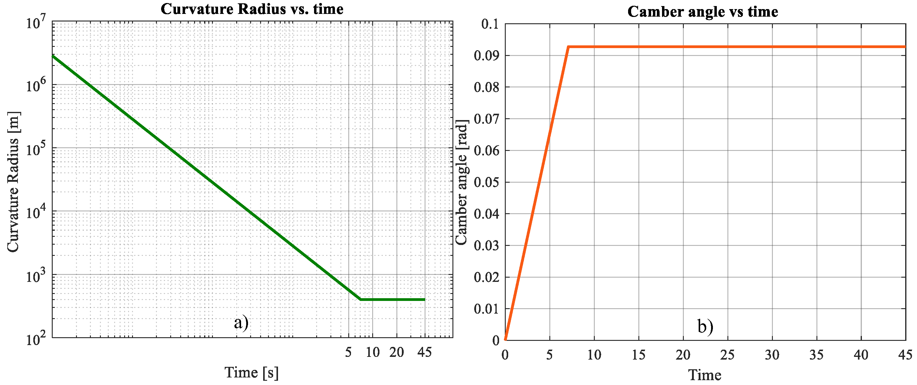
In this study, a trajectory composed of three paths (a straight path, a path of variable radius of curvature and a path of constant curvature) is modeled. For simulation purposes, only geometric variations are considered in order to obtain the values of the adherence and normal forces present, while a vehicle follows a simulation trajectory composed of these three paths with a different radius of curvature. This design fits to realistic transport routes since it has been calculated and parameterized with curves of agreement (trajectories that connect a straight and circular trajectory in such a way that it starts with an infinite radius of curvature and ends in a constant radius of curvature) used in road design.

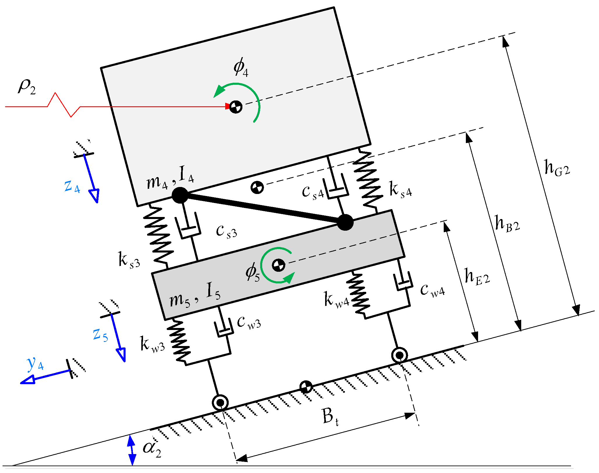
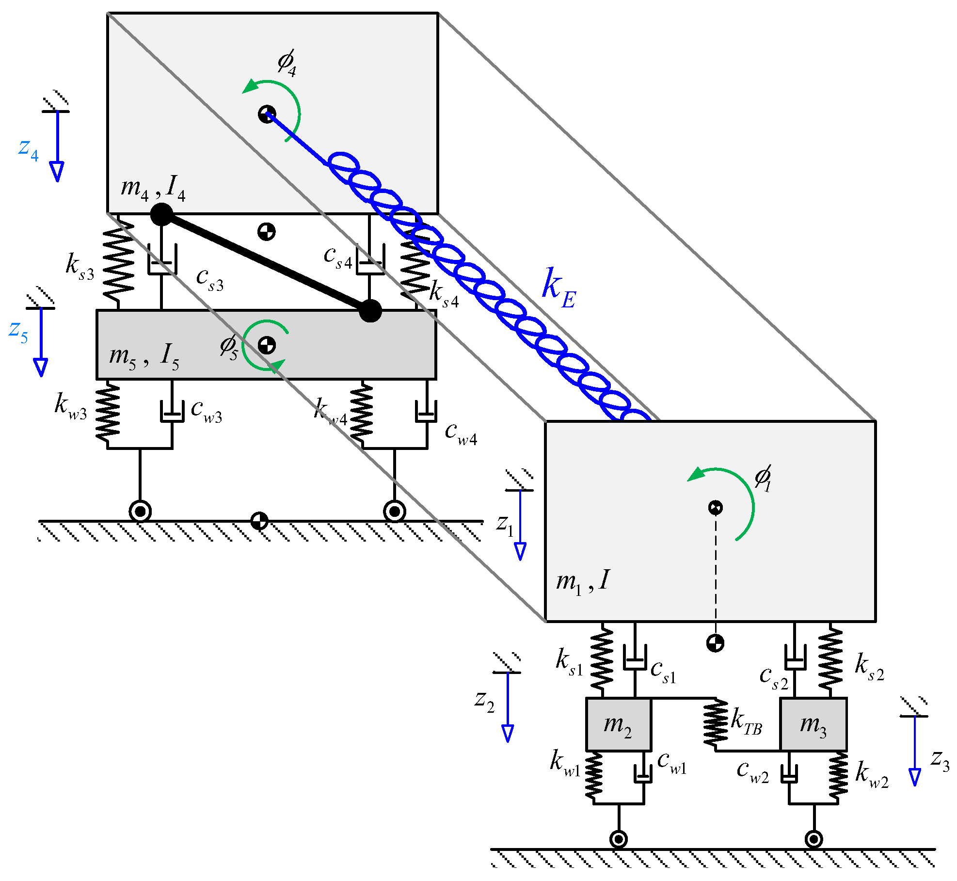
A bus model is provided using rigid multibody systems with which a virtual or mathematical model (system of ordinary differential equations) has been generated. The passenger bus is then modeled in two sections, front and rear. The front part contemplates several subsystems, such as the unsprung masses, the unsprung masses are connected by a stability or torsion bar, the flexible wheels, etc. These parts are represented by a set of inertia, stiffness, and damping elements. The rear part has been modeled in an analogous way although, unlike the front, in this there is only one unsprung mass and a Panhard type bar is used to improve its vertical and lateral dynamic behavior. For this model, the suspension system and tire stiffness as well as the damping of both bodies have been modeled as linear components.

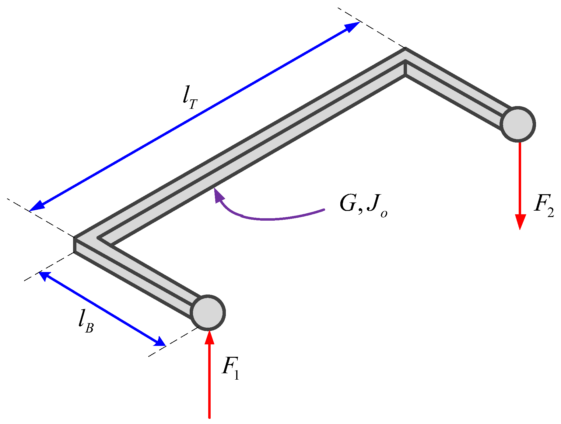
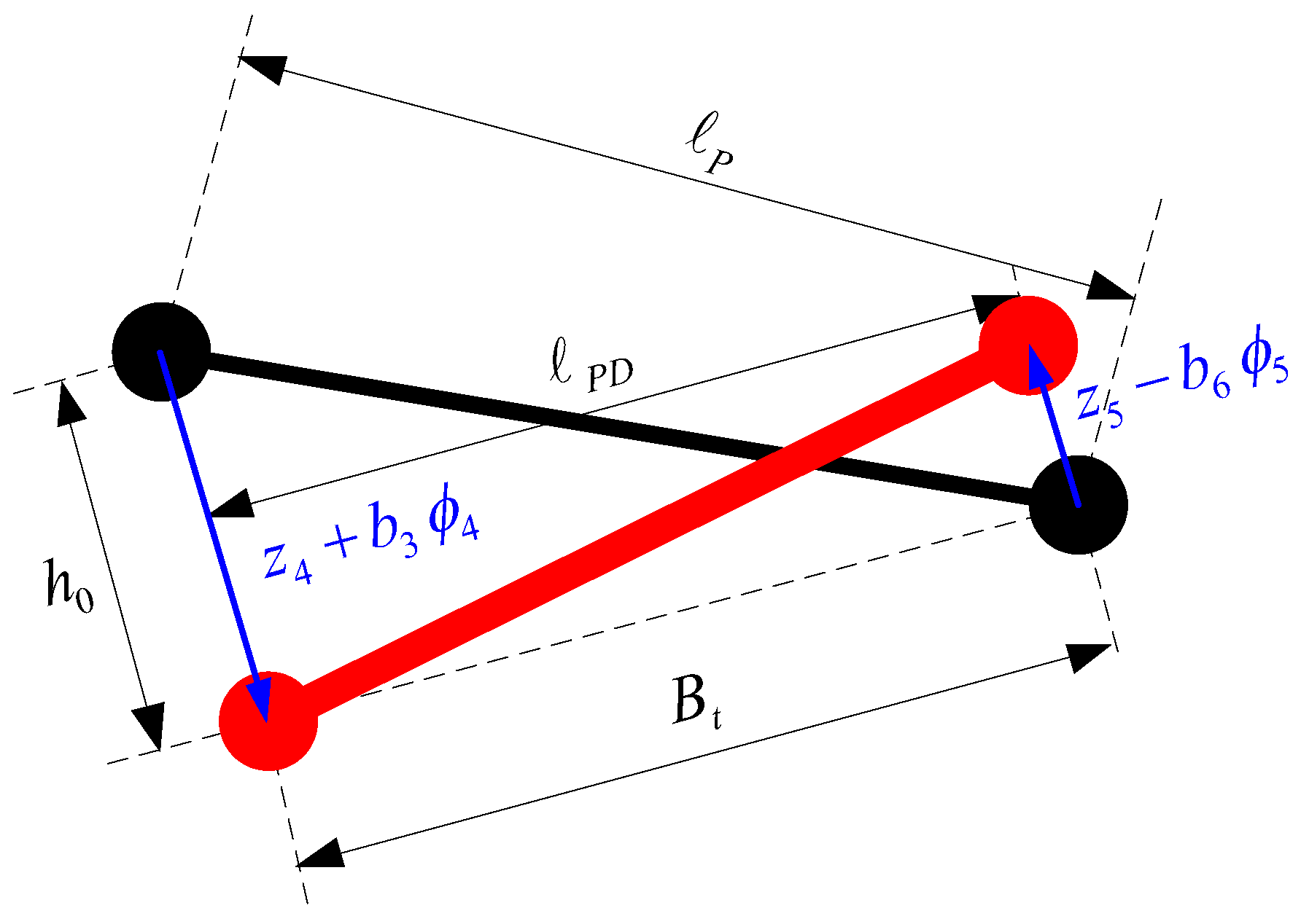
The Panhard bar is a suspension element that prevents lateral displacements of an axle and also restricts the relative vertical movement between the suspended and unsuspended mass. Independent rear suspension systems do not require a Panhard bar. The bar is attached to two points that allow only the up and down movement of its ends, so that it can only move in the vertical plane. The forces that restrict the movement between the connected elements take part in the dynamics of these, since the forces and the consequent moments that originate, both in the non-suspended mass and in the suspended, intervene in their dynamics. Some previous studies have incorporated a Panhard bar in their vehicle models. In [17], a roll plane model of a road vehicle is provided incorporating the kinematic constraint provided by a Panhard bar. The results show that the location and orientation of the Panhard bar significantly influences the kinetostatic roll properties of the suspension when the vehicle is subjected to vertical and lateral forces. In [18], a common front axle suspension is designed for four different tractor models, in which a Panhard bar is used to improve safety and driving stability. Related with the Panhard bar [19], it compares the structural durability behavior of commercial vehicles Panhard bars of a ferritic cast nodular iron with the behavior of rods of an austempered.

Both sections of the bus are connected by a torsional spring (defined by its torsional stiffness) to emulate the dynamic influence of the vehicle chassis. Due to the different longitudinal position of the two sections and, consequently, the different roll angle, the chassis exerts a torsional moment on both sections, which influences the lateral stability.

This bus model travels along the simulated trajectory and allows the simulation of the lateral dynamics of a bus when it travels on a cambered curve.

2. Geometric Path Description

In Figure 1, a schematic model of the path considered for this work is shown.

These dimensions are subsequently applied to modeling of the road, with the radius of curvature $\rho$ and camber angle $\alpha$ as geometric parameters defining the dynamic behavior of the vehicle on a curved path. The track’s width $B_t$ and roadway width $B_w$ define the maximum value of the camber height and the vehicle width, respectively; the track width also defines the number of lanes on the road. In order to simplify the simulation, it has been assumed that the vehicle is driving in the middle roadway lane.

2.1. Kinematic Effects

The radius of curvature of a track section measures the magnitude of the curvature in that section. According to the formulation deduced by dynamics, the normal acceleration a_y, caused by said curvature, is defined by the following equation:

$$a_y=v^2/\rho$$

(1)

This acceleration, mainly dependent on the speed (v) and inversely proportional to the radius of curvature, is translated into an inertial force, opposite in sense to the normal acceleration and oriented on the horizontal of the plane in which it is located. This inertial force is commonly known as centrifugal force, F_i:

$$F_i=\frac{v^2}{\rho }{m}_T$$

(2)

where m_T is the total mass of the vehicle.

The camber is defined as a relative elevation between the ends of the track, such that a component of the vehicle’s weight compensates the inertial force caused by normal acceleration; its length is measured between the ends of the track according to the vertical direction (Figure 1).

Figure 2 shows a resultant force R as the vectorial sum of the weight and inertial force (centrifugal force). As an effect of the inclination, there is a component of this resultant force, which is perpendicularly pointed to the path’s plane $R_N$, which keeps an adherence force between the wheel and the path, and a perpendicular oriented component $R_T$ of the resultant force R, which is responsible for the skidding and rollover of the vehicle; when the resultant force R is completely oriented in the perpendicular direction of the path’s plane, it is said that the vehicle is traveling at design velocity $v_D$.

For a skidding situation, it is said that the parallel component of R force is higher than the adherence force determined by the Coulomb’s dry friction force; on the other hand, when a rollover is produced, the vehicle will turn into the external side of the curve, it means that it will turn over one or more wheel from the external side of the vehicle. Consequently, we can affirm that when the normal force of one or more wheels in the inner side are zero the rollover is produced, or is at least imminent. To analyze the vehicles rollover, a fixed point is required thus the concept of roll center is introduced as a reference point, which despite the strains that suspension suffers, it remains static on the vehicle frontal plane. From this point, all moments are calculated so it is important to highlight that the higher the vehicle’s mass center, the higher the possibility of rollover.

2.2. Kinds of Path

Three path types with different geometric characteristics (curvature radius and camber) have been defined as shown in

Table 1. Geometrical characteristic variations for type of path.

Type of Path	Camber Angle	Curvature Radius
Straight path	None	Infinite
Transition path	Variable	Variable
Circular path	Constant	Constant

.

The transition curves enhance the horizontal curve safety as they help to gradually apply camber and centrifugal force. Since the transition path is the only one which varies its parameters, it is the only one that defines parameter variation equations. Such paths connect a straight and a circular path so that begins with an infinite curvature radius and ends at a constant curvature radius; furthermore, over those paths, the camber angle starts to increase or decrease. To describe those paths a variety of mathematical curves are applied to determine their points in the space. Among those curves, the most known are Bernoulli’s lemniscate and the clothoid, which is the most widely applied [15]. The use of a clothoid transition curve between tangent and a circular curve has been suggested to increase the safety margin of safety against sideslip, especially when the camber exceeds 12% [20]. So, the clothoid has been used in this study.

A clothoid is defined by the following equation:

$$\rho \left(s\right)\cdot s=A^2$$

(3)

where s is the traveled distance over the curve and $\rho \left(s\right)$ is the curvature radius as a function of the traveled distance, it means that there is a linear correspondence through a constant. This could be interpreted as while the vehicle is moving forward over the path, the magnitude of the curvature radius increases or decreases. A clothoid curve is depicted in Figure 3.

The position vector is described by the following equation which is expressed in terms of Fresnel functions:

$$\overrightarrow{r}(s)=\left[x(s);y(s)\right]=A\sqrt{\pi }\left[\mathrm{FresnelC}\left(\frac{s}{A\sqrt{\pi }}\right);\mathrm{FresnelS}\left(\frac{s}{A\sqrt{\pi }}\right)\right]$$

(4)

One of the most important functions is avoid the appearance of sudden uncompensated acceleration, thus it is required to evaluate the magnitude of the over acceleration, which is the rate of variation of the acceleration. According to [21], for railway vehicles, it is recommended that this value must not overcome 0.2 m/s³; nevertheless, for a road vehicle, this value should be controlled by the maneuvering of the car’s rudder. For this simulation, this value must be settled as an input parameter, hence the maneuvering of the vehicles is not being simulated as it is a random parameter.

2.3. Simulation Path Parameterization

Once all geometric characteristics of the path are known, it is necessary to build, in a parametric way, the simulation path over which the vehicle will travel during the simulation. For that reason, the following equations are developed to describe the camber and curvature radiuses over the clothoid:

$$\rho \left(t\right)=\frac{A^2}{v\left(t\right)t}$$

(5)

$$z\left(t\right)=v\left(t\right)t\frac{z_b}{s_b}$$

(6)

In the previous expressions, $z_b$ is the constant camber value in the circular path and $s_b$ is the total length of the clothoid. The velocity is going to be considered as a constant value for simulation path generation purpose. Due to the vehicle’s behavior is studied just a transition and circular path are required, hence in a straight path there is no risk of rollover because lateral acceleration is not present.

From Equation (6) an equivalence to determine $s_{b,\min }$ clothoid curve minimum length can be calculated. According with [21], the maximum noncompensated lateral acceleration should be 1 m/s² for comfort and safety reasons. From the given conditions, the following expression can be developed:

$$\frac{\left(\frac{9.81 z_b}{B_{\mathrm{w}}}-\frac{v^2\sqrt{B_w^2-z_b{}^2}}{{\rho }_{\min } B_w}\right)v_D}{0.2}<s_{b,\min }$$

(7)

From this expression, the clothoid’s constant can be determined:

$$A=\sqrt{s_{b,\min }{\rho }_b}$$

(8)

Once the transition path is defined, a circular path can be added giving as a result the whole simulation path.

For this work, a simulation path was developed considering the following parameters:

• Camber over the circular path (Final value): 0.25 m
• Curvature radius over the circular path (Final value): 400 m
• Track’s width: 0.9 m
• Number of tracks: 3
• Maximum over acceleration: 0.15 m/s³
• Path’s total length: 1500 m
• Average Speed: 120 km/h

Figure 4 shows a plane view of the track and the center of the circular path:

Taking as a reference the average speed, function for camber angle and curvature radius can be developed in terms of time (Figure 5).

3. Vehicle Modeling

As it has been described, to simplify the vehicle analysis, the bus has been divided into two sections, front and rear, both are joined by a torsional spring, which emulates the stiffness belonging to the bus structure.

3.1. Frontal Section

For the front section, the unsprung mass includes elements, such as the mass of the tires and other components of the steering system, all of them are modelled as punctual masses, which have only one degree of freedom on the perpendicular direction of path’s plane. The Figure 6 shows the theoretical representation of the front section of the bus:

The model proposed is based on [22,23]. This model considers not only the stiffness of the wheels but also the damping of that element so that it is possible to get a more realistic bus mechanical behavior. Additionally, a sway bar is considered as passive element, this component has the functionality of link the vertical displacement of the unsprung masses. It is performed taking advantage of the lever arms generated by the displacement giving as a result a torsional moment along the bar so that restrict the movement of both unsprung masses, it is desirable to avoid excessive vibrations, as well as a large displacement of the roll center.

3.2. Rear Section

In the rear section, the unsprung mass is modeled as a unique body, which is linked with the bus chassis through the suspension system so that the unsprung mass has two degrees of freedom, the vertical displacement, and a rotation around the longitudinal axis. Most of the components are quite like the front section except for a rigid element known as a Panhard bar which, as mentioned above, is used to avoid lateral displacement, and restrict relative vertical displacement and rotation between the unsprung and sprung masses. In terms of modeling, the Panhard bar is considered to be embedded in the unsprung mass and articulated to the sprung mass.

A model of the rear section is depicted in Figure 7.

Regarding the camber angle and curvature radius, the values of both parameters are different from the front section, hence they are in different positions over the path; for that reason, a time interval delay is introduced to simulate that effect.

3.3. Complete Model

From the aforementioned description, a torsional spring, with a torsional stiffness $k_E$ that links both sections to emulate the stiffness of the bus structure chassis. Altogether, an 8 degree of freedom model is composed by the two sections. The whole model is shown in Figure 8.

4. Kinetic Analysis of the Vehicle

4.1. Frontal Section

Hence, the forces on some vehicle components will be analyzed and a few parameters will be modified to study the influence it has on behavior, the motion equations are going to be determined by applying the D’Alembert principle. Firstly, equations belonging to the suspended mass are obtained and then the equations corresponding to the unsprung masses.

From the geometric parameters of the road, which has been previously described, it is possible to notice that the horizontal acceleration is the known centripetal acceleration produced by the vehicle’s travel over a curved road, therefore the only unknown acceleration is vertical acceleration. Both accelerations can be decomposed into two orthogonal components, one parallel and the other normal to the road plane (Figure 9). Transposing those accelerations to the equivalent system and analyzing the so-called dynamic equilibrium, motion equations are going to be obtained.

Suspended mass rotation, its angular speed and its vertical displacement are responsible for the forces on the suspension’s system components and each of them is linked to the displacement of the correspondent unsprung mass connected to them. From those forces and considering the center of gravity location, the moments around its roll center can be calculated. In Figure 10, the front of the body diagram for dynamic equilibrium is shown.

From the free body diagram, the following differential equations are settled. For the vertical displacement $z_1$:

$$\begin{array}{l}{m}_1{\ddot{z}}_1=-\left[k_{s1}(z_1+b_1 {\varphi }_1-z_2)+c_1({\dot{z}}_1+b_1 {\dot{\varphi }}_1-{\dot{z}}_2)\right]\\ \hspace{1em}\hspace{1em}\hspace{1em}- \left[k_{s2}(z_1-b_2 {\varphi }_1-z_3)+c_2({\dot{z}}_1-b_2 {\dot{\varphi }}_1-{\dot{z}}_3)\right]\\ \hspace{1em}\hspace{1em}\hspace{1em}+\frac{m_1{v}^2}{{\rho }_1\left(t\right)}\sin \left[{\alpha }_1\left(t\right)+{\varphi }_1\left(t\right)\right]\end{array}$$

(9)

For rotation ${\varphi }_1$:

$$\begin{array}{c}\left[I_1+m_1{\left(h_{G1}-h_{B1}\right)}^2\right]{\ddot{\varphi }}_1=b_2\left[k_{s2}(z_1-b_2{\varphi }_1-z_3)+c_2({\dot{z}}_1-b_2{\dot{\varphi }}_1-{\dot{z}}_3)\right]\\ -b_1\left[k_{s1}(z_1+b_1{\varphi }_1-z_2)+c_1({\dot{z}}_1+b_1{\dot{\varphi }}_1-{\dot{z}}_2)\right]\\ -\left[\left(m_1\frac{v^2}{{\rho }_1\left(t\right)}\cos \left({\alpha }_1\left(t\right)+{\varphi }_1\left(t\right)\right)\right)\left(h_{G1}-h_{B1}\right)\right]\\ +\left[\left(m_{1}g\sin {\alpha }_1\left({\alpha }_1\left(t\right)+{\varphi }_1\left(t\right)\right)\right)\left(h_{G1}-h_{B1}\right)\right]+T_{est}\end{array}$$

(10)

This equation considers a resistant torque, which is caused by the torsional stiffness of the vehicle’s structure; said moment is denoted by $T_{est}$, which will be determined later. For the unsprung masses, the analysis is quite similar as that carried out for the suspended mass, with the difference of the intervention of the torsion bar, which links the movements of both suspended masses. Figure 11 shows the free body diagram and equivalent system of both unsprung masses.

In Figure 11, it is possible to note that there is a force produced by the sway bar $F_{TB}$, which is opposite at each unsprung mass. This element takes advantage of the lever arms generated by each unsprung mass, which due to the displacement difference between the ends of the bar generates a torsion moment.

The displacement can be calculated as follow:

$$z_2=\frac{F_1{l}_b^3}{3E_b{I}_b}$$

(11)

where $F_1$ is the force applied by the left unsprung mass, $l_b$ is the arm bar’s length, $E_b$ Young Modulus of the bar material and $I_b$ is the bar’s inertia moment. The force applied at each end of the bar can be determined by the following equation:

$$F_1\left(z_2\right)=\frac{3z_2{E}_b{I}_b}{l_b^3}$$

(12)

From Equation (12), a correlation between unsprung mass displacements and force in the bar can be obtained. Figure 12 shows the free body diagram of the sway bar.

From the force calculated in (12), the torsion moment over the bar is calculated:

$$M_{t1}=F_1{l}_b=\frac{3z_2 E_b{I}_b}{l_b^2}$$

(13)

In a similar way, it is possible calculate the moment generated by the unsprung right mass as follow:

$$M_{t2}=F_2{l}_b=\frac{3z_3 E_b{I}_b}{l_b^2}$$

(14)

Due to the moment exerted by both arms being opposite, the resultant torsion moment is calculated from the difference between them:

$$M_{TB}=M_{t1}-M_{t2}=\frac{3 E_b{I}_b}{l_b^2}\left(z_2-z_3\right)$$

(15)

The resultant torsion moment generates a rotation angle on the bar:

$${\mathsf{\Phi }}_B=\frac{M_{TB} l_T}{G J_0}$$

(16)

This angle can be related to the displacement arm difference as follows:

$$z_{\Delta }=z_{\Delta }=\mathsf{\Phi } l_b=\frac{3 E_b{I}_b l_T}{l_b G J_0}\left(z_2-z_3\right)$$

(17)

From Equation (17) and due to the linear correlation between the displacement and the unsprung mass displacements, an elastic constant is determined:

$$k_{tb}=\frac{9 E_b^2{I}_b^2 l_T}{l_b^4 G J_0}$$

(18)

Considering the influence of the sway bar and applying the acceleration decomposition and transposing them to the first member of the equivalence (Dynamic equilibrium), the following motion equations are developed:

Unsprung left mass:

$$\begin{array}{l}{m}_2 {\ddot{z}}_2-m_2\frac{v^2}{{\rho }_1\left(t\right)}\sin \left[{\alpha }_1\left(t\right)+{\varphi }_1\left(t\right)\right]=k_{s1}(z_1+b_1 {\varphi }_1-z_2)+c_1({\dot{z}}_1+b_1 {\dot{\varphi }}_1-{\dot{z}}_2)\\ -k_{TB}\left(z_2-z_3\right)-k_{w1} z_2-c_{w1} {\dot{z}}_2\end{array}$$

(19)

Unsprung right mass:

$$\begin{array}{l}{m}_3 {\ddot{z}}_3=k_{s2}(z_1-b_1 {\varphi }_1-z_3)+c_2({\dot{z}}_1-b_1 {\dot{\varphi }}_1-{\dot{z}}_3)\\ +k_{TB}(z_2-z_3)-k_{w2} z_3-c_{w2} {\dot{z}}_3\\ +m_3\frac{v^2}{{\rho }_1\left(t\right)}\sin [{\alpha }_1(t)+{\varphi }_1(t)]\end{array}$$

(20)

4.2. Rear Section

In a similar way as the front section, the free body diagram of the suspended mass for dynamic equilibrium is depicted in Figure 13.

In comparison with the front section, here there is a noticeable effect of the Panhard bar, which is represented by the forces $F_{Ph}$ and $F_{Pv}$, which are the horizontal and vertical component of the force along the bar. Additionally, for the acceleration decomposition, the influence of the rotation angle of both masses, unsprung and suspended, must be taken into account, including the torsional torque produced by the structure. From this and the free body diagram the following motion equations are obtained:

For the displacement $z_4$

$$\begin{array}{l}{m}_4\left({\ddot{z}}_4-\frac{v^2}{{\rho }_2\left(t\right)}\sin \left[{\alpha }_2\left(t\right)+{\varphi }_4\left(t\right)+{\varphi }_5\left(t\right)\right]\right)=-k_{s3}\left(z_4+b_3{\varphi }_4-z_5-b_5{\varphi }_5\right)\\ -k_{s4}\left(z_4-b_4{\varphi }_4-z_5+b_6{\varphi }_5\right)\\ -c_{s3}({\dot{z}}_4+b_3{\dot{\varphi }}_4-{\dot{z}}_5-b_5{\dot{\varphi }}_5)\\ -c_{s4}({\dot{z}}_4-b_4{\dot{\varphi }}_4-{\dot{z}}_5+b_6{\dot{\varphi }}_5)+F_{Pv}\end{array}$$

(21)

For the rotation ${\varphi }_4$:

$$\begin{array}{l}\left[I_4+m_4{\left(h_{G2}-h_{B2}\right)}^2\right]{\ddot{\varphi }}_4=b_4\left[k_{s4}(z_4-b_4{\varphi }_4-z_5+b_6{\varphi }_5)+c_{s4}({\dot{z}}_4-b_4{\dot{\varphi }}_4-{\dot{z}}_5+b_6{\dot{\varphi }}_5)\right]\\ -b_3\left[k_{s3}(z_4+b_3{\varphi }_4-z_5-b_5{\varphi }_5)+c_{s3}({\dot{z}}_4+b_3{\dot{\varphi }}_4-{\dot{z}}_5-b_5{\dot{\varphi }}_5)-F_{Pv}\right]\\ -\left[\left(m_4\frac{v^2}{{\rho }_2\left(t\right)}\cos \left[{\alpha }_2\left(t\right)+{\varphi }_4\left(t\right)+{\varphi }_5\left(t\right)\right]\right)\left(h_{G2}-h_{B2}\right)\right]-T_{est}\\ +\left[\left(m_{4}g\sin \left[{\alpha }_2\left(t\right)+{\varphi }_4\left(t\right)+{\varphi }_5\left(t\right)\right]\right)\left(h_{G2}-h_{B2}\right)\right]\\ -\left[F_{Ph}\left(h_{G2}-h_{S2}-h_{B2}\right)\right]\end{array}$$

(22)

For the unsprung mass, the analysis is similar obtaining the free body diagram for the dynamic equilibrium showed in Figure 14.

From the free body diagram, the following motion equations are obtained:

For the displacement $z_5$

$$\begin{array}{l}{m}_5{\ddot{z}}_5=-k_{w3}(z_5+b_5{\varphi }_5)-c_{w3}({\dot{z}}_5+b_5{\dot{\varphi }}_5)-k_{w4}(z_5-b_6{\varphi }_5)\\ -c_{w4}({\dot{z}}_5-b_6{\dot{\varphi }}_5)+k_{s3}(z_4+b_3{\varphi }_4-z_5-b_5{\varphi }_5)\\ +k_{s4}(z_4-b_4{\varphi }_4-z_5+b_6{\varphi }_5)+c_{s3}({\dot{z}}_4+b_3{\dot{\varphi }}_4-{\dot{z}}_5-b_5{\dot{\varphi }}_5)\\ +c_{s4}({\dot{z}}_4-b_4{\dot{\varphi }}_4-{\dot{z}}_5+b_6{\dot{\varphi }}_5)-F_{Pv}+\frac{m_5{v}^2}{{\rho }_2\left(t\right)}\sin ({\alpha }_2\left(t\right)+{\varphi }_5\left(t\right))\end{array}$$

(23)

For the rotation ${\varphi }_5$:

$$\begin{array}{l}\left[I_5+m_5{(h_{E2})}^2\right]{\ddot{\varphi }}_5=b_6\left[\begin{array}{l}{k}_{w4}(z_5-b_6{\varphi }_5)+c_{w4}({\dot{z}}_5-b_6{\dot{\varphi }}_5)\\ -k_{s4}(z_4-b_4{\varphi }_4-z_5+b_6{\varphi }_5)\\ -c_{s4}({\dot{z}}_4-b_4{\dot{\varphi }}_4-{\dot{z}}_5+b_6{\dot{\varphi }}_5)+F_{PB}\end{array}\right]\\ -b_5\left[\begin{array}{l}{k}_{s3}(z_4+b_3{\varphi }_4-z_5-b_5{\varphi }_5)\\ +c_{s3}({\dot{z}}_4+b_3{\dot{\varphi }}_4-{\dot{z}}_5-b_5{\dot{\varphi }}_5)\\ -k_{w3}(z_5+b_5{\varphi }_5)-c_{w3}({\dot{z}}_5+b_5{\dot{\varphi }}_5)\end{array}\right]\\ +h_{E2}\left[\begin{array}{l}\left(m_{5}g\sin \left[{\alpha }_2\left(t\right)+{\varphi }_5\left(t\right)\right]\right)-\\ \left(m_5\frac{v^2}{{\rho }_2\left(t\right)}\cos [{\alpha }_2\left(t\right)+{\varphi }_5\left(t\right)]\right)+F_{Ph}\end{array}\right]\end{array}$$

(24)

The forces produced by the Panhard bar require a kinematic analysis of both ends of it. Such a component could be modeled as a bar element on which its inner force acts along itself, therefore the force’s direction is already known.

Considering only the vertical displacement at the ends of the bar, Figure 15 shows the displacement of each point connected to the Panhard bar:

From that displacement, the bar vertical displacement can be analyzed as it is shown in Figure 16.

From this analysis, the vertical dimension of the bar can be calculated as follow:

$$h=h_0+z_5-b_6{\varphi }_5-z_4-b_3{\varphi }_4$$

(25)

With the vertical dimension determined, the bar’s length can be calculated directly:

$${{\displaystyle \mathcal{l}}}_{PD}=\sqrt{ h_{}^2+B_t^2}$$

(26)

Additionally, its orientation:

$${\phi }_B=\arctan \left(\frac{B_t}{h_0+z_5-b_6{\varphi }_5-z_4-b_3 {\varphi }_4}\right)$$

(27)

Later, the bar stiffness can be calculated instantly as follow:

$$k_P=\frac{EA}{{{\displaystyle \mathcal{l}}}_{PD}}$$

(28)

where E is the material’s Young Modulus and A its transversal area.

As a final step the influence of the torsional stiffness of the structure is seen on the motion equations, so the torsional moment originated this element is equivalent to the following expression:

$$T_{est}=k_E\left({\varphi }_4-{\varphi }_1\right)$$

(29)

This component links both bus sections, so all differential equations developed are coupled.

5. Simulation and Results

Due to the complexity of the model, a state space model must be implemented, so that the motion equations settled previously can be arranged as a differential equation system, which can be divided into two matrices, one as a state matrix $A$ which is entirely lineal, and an input matrix $B$, which due to the Panhard bar and its dependency to the variable states is highly non-lineal.

From the state space equation:

$$\begin{array}{c}dx=Ax+Bu\\ y=Cx+Du\end{array}$$

(30)

The state vector is defined as follow:

$$x=\left[\begin{array}{cccccccccccccccc}{z}_1& {\dot{z}}_1& z_2& {\dot{z}}_2& z_3& {\dot{z}}_3& {\varphi }_1& {\dot{\varphi }}_1& z_4& {\dot{z}}_4& z_5& {\dot{z}}_5& {\varphi }_4& {\dot{\varphi }}_4& {\varphi }_5& {\dot{\varphi }}_5\end{array}\right]$$

(31)

Due to its dimensions and simplicity, the state matrix which is a 16 × 16 square matrix will not be shown on this document, but the input matrix will be presented for its non-linear formulation:

$$\left(\begin{array}{c}0\\ \frac{v^2}{\rho \left(t\right)}\sin \left(\alpha \left(t\right)+{\varphi }_1\right)\\ 0\\ \frac{v^2}{\rho \left(t\right)}\sin \alpha \left(\alpha \left(t\right)+{\varphi }_1\right)\\ 0\\ \frac{v^2}{\rho \left(t\right)}\sin \alpha \left(\alpha \left(t\right)+{\varphi }_1\right)\\ 0\\ \frac{-\left(m_1\frac{v^2}{\rho \left(t\right)}\cos \left(\alpha \left(t\right)+{\varphi }_1\right)\right)\left(h_{G1}-h_{B1}\right)+\left(m_{1}g\sin \left(\alpha \left(t\right)+{\varphi }_1\right)\right)\left(h_{G1}-h_{B1}\right)}{I_{1B}}\\ 0\\ \frac{v^2}{\rho \left(t-1\right)}\sin \left(\alpha \left(t-1\right)+{\varphi }_4+{\varphi }_5\right)+\frac{F_{Pv}}{m_4}\\ 0\\ \frac{v^2}{\rho \left(t-1\right)}\sin \left(\alpha \left(t-1\right)+{\varphi }_5\right)-\frac{F_{Pv}}{m_5}\\ 0\\ \frac{\left(\begin{array}{l}-m_4\frac{v^2}{\rho \left(t-1\right)}\cos \left(\alpha \left(t-1\right)+{\varphi }_4+{\varphi }_5\right)\\ +m_{4}g\sin \left(\alpha \left(t-1\right)+{\varphi }_4+{\varphi }_5\right)\end{array}\right)\left(h_{G2}-h_{B2}\right)-F_{Ph}\left(h_{S2}\right)+F_{Pv}{b}_3}{I_{4B}}\\ 0\\ \frac{\left[\left(m_{5}g\sin \left(\alpha \left(t-1\right)+{\varphi }_5\right)\right)-\left(m_5\frac{v^2}{\rho \left(t-1\right)}\cos \left(\alpha \left(t-1\right)+{\varphi }_5\right)\right)+F_{Ph}\right]h_{E2}+F_{Pv}{b}_6}{I_{5B}}\end{array}\right)$$

(32)

From the equations given in this matrix, it is highly dependent on the state matrix so that matrix B is a function of x. Although there is a control vector u and matrix C, output, and matrix D, feedforward, this matrix will be replaced by an identity matrix and a row vector with ones, hence the main purpose of the settled system is simulation. In further works, this matrix can be replaced to obtain a control system. All equations for the path and other elements, such as a Panhard bar, are modeled in a Simulink^® algorithm.

Once the differential equations are expressed into the state space equation, it is necessary to numerically fix all the mechanic parameters which have been taken from [24] are expressed in the following list:

$m_1=7000 \mathrm{kg}$—Front suspended mass

$m_2=500 \mathrm{kg}$—Front left unspring mass

$m_3=500 \mathrm{kg}$—Front right unspring mass

$I_1=125,000 \mathrm{kg}\cdot {\mathrm{m}}^2$—Front suspended mass inertia respect to its mass center

$c_1=600 \mathrm{N}\cdot \mathrm{s}/\mathrm{m}$—Damping coefficient of the left front suspension element

$c_2=600 \mathrm{N}\cdot \mathrm{s}/\mathrm{m}$—Damping coefficient of the right front suspension element

$b_1=0.8 \mathrm{m}$—Distance from suspended mass center to the left front suspension

$b_2=0.8 \mathrm{m}$—Distance from suspended mass center to the right front suspension

$k_{s1}=200,000 \mathrm{N}/\mathrm{m}$—Stiffness coefficient of the left front suspension element

$k_{s2}=200,000 \mathrm{N}/\mathrm{m}$—Stiffness coefficient of the right front suspension element

$h_{B1}=0.75 \mathrm{m}$—Roll center front suspended mass height respect to the path’s plane.

$h_{G1}=1.55 \mathrm{m}$—Mass center height of the suspended front mass

$k_{TB}=1,000,000 \mathrm{N}/\mathrm{m}$—Stiffness coefficient of the sway bar

$k_{w1}=921,607 \mathrm{N}/\mathrm{m}$—Stiffness coefficient of the front left tire

$k_{w2}=921,607 \mathrm{N}/\mathrm{m}$—Stiffness coefficient of the front right tire

$c_{w1}=800 \mathrm{N}\cdot \mathrm{s}/\mathrm{m}$—Damping coefficient of the front left tire

$c_{w2}=800 \mathrm{N}\cdot \mathrm{s}/\mathrm{m}$—Damping coefficient of the front right tire

$k_E=600,000,000 \mathrm{N}\cdot \mathrm{m}/\mathrm{rad}$—Torsional stiffness coefficient of the vehicle structure

$m_4=7000 \mathrm{kg}$—Read suspended mass

$m_5=1000 \mathrm{kg}$—Rear left unspring mass

$I_4=125,000 \mathrm{kg}\cdot {\mathrm{m}}^2$—Rear suspended mass inertia respect to its mass center

$I_5=1000 \mathrm{kg}\cdot {\mathrm{m}}^2$—Rear unspring mass inertia respect to its mass center

$c_3=600 \mathrm{N}\cdot \mathrm{s}/\mathrm{m}$—Damping coefficient of the left rear suspension element

$c_4=600 \mathrm{N}\cdot \mathrm{s}/\mathrm{m}$—Damping coefficient of the right rear suspension element

$b_3=0.8 \mathrm{m}$—Distance from suspended mass center to the left rear suspension

$b_4=0.8 \mathrm{m}$—Distance from suspended mass center to the right rear suspension

$b_5=0.8 \mathrm{m}$—Distance from unspring mass center to the left rear tire

$b_6=0.8 \mathrm{m}$—Distance from unspring mass center to the right rear tire

$k_{s3}=200,000 \mathrm{N}/\mathrm{m}$—Stiffness coefficient of the left rear suspension element

$k_{s4}=200,000 \mathrm{N}/\mathrm{m}$—Stiffness coefficient of the right rear suspension element

$h_{B2}=0.75 \mathrm{m}$—Roll center rear suspended mass height respect to the path’s plane.

$h_{G2}=1.55 \mathrm{m}$—Mass center height of the suspended rear mass

$h_{E2}=0.5 \mathrm{m}$—Mass center height of the unspring rear mass

$k_{w3}=921,607 \mathrm{N}/\mathrm{m}$—Stiffness coefficient of the rear left tire

$k_{w4}=921,607 \mathrm{N}/\mathrm{m}$—Stiffness coefficient of the rear right tire

$c_{w3}=800 \mathrm{N}\cdot \mathrm{s}/\mathrm{m}$—Damping coefficient of the rear left tire

$c_{w4}=800 \mathrm{N}\cdot \mathrm{s}/\mathrm{m}$—Damping coefficient of the rear right tire

Also, for the Panhard bar, the following parameters are taken:

$E=2.1\times {10}^5{ \mathrm{N}/\mathrm{mm}}^2$—Panhard bar material’s Young modulus

$d_P=30 \mathrm{mm}$—Panhard bar diameter

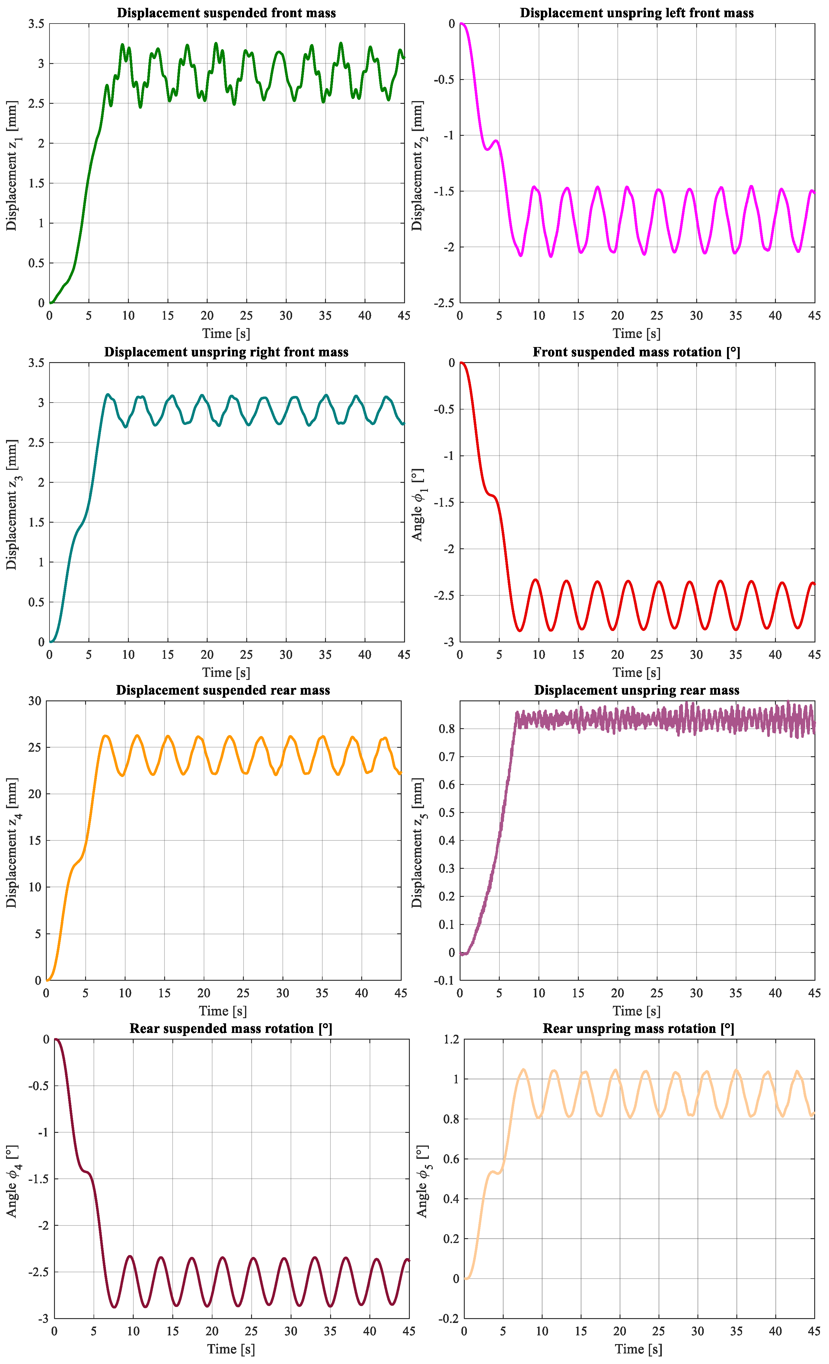
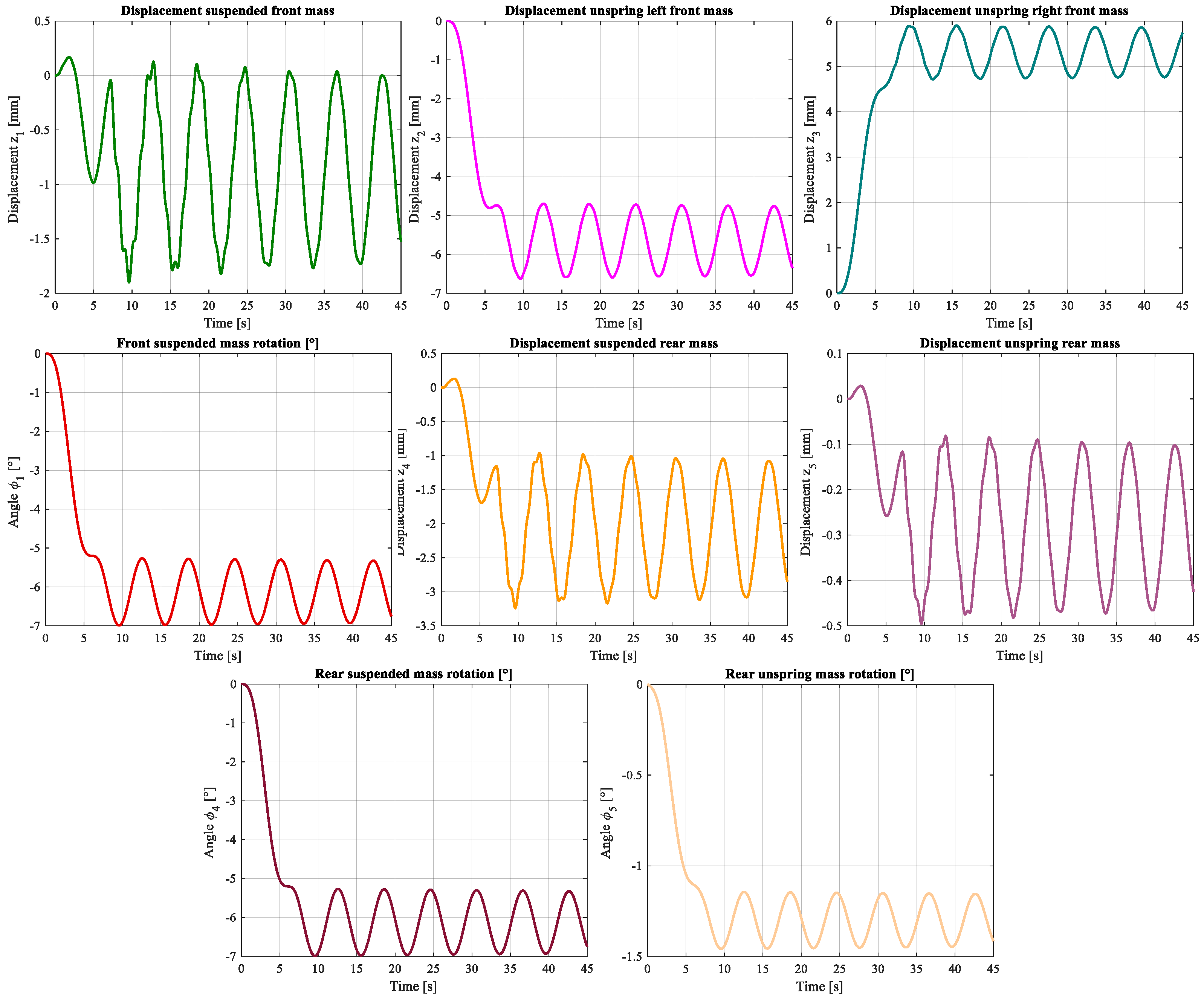
From the constants given above, the following results are obtained from the simulation of the vehicle’s travel over a transition and circular path, as previously given (Figure 17).

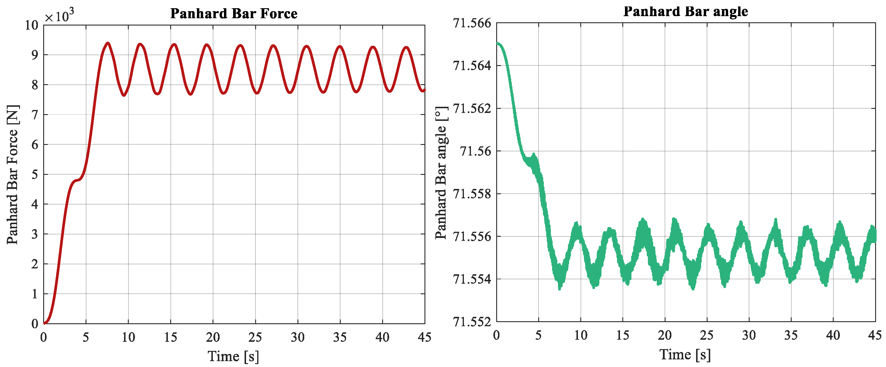
Furthermore, the instantaneous Panhard’s bar force and angle are also obtained from the simulation (Figure 18).

Those results show the bus dynamic behavior when it is traveling over a transition and circular curve; in fact, it is noticeable that while the bus is over the clothoid its position and rotation state variables are increasing constant and when it arrives at the circular path they become oscillating, consequently, the Panhard bar length and angle have the same behavior.

5.1. Effects of the Panhard Bar

The addition of the Panhard bar has a stabilization function on the mechanical behavior of the bus, the main effect is appreciated on the rear mass rotation angles, which have an effect on the displacements and angles in the front section. It can be said that the Panhard bar shrinks the oscillations of each state variable as can be appreciated, making a comparison between Figure 17 and Figure 19.

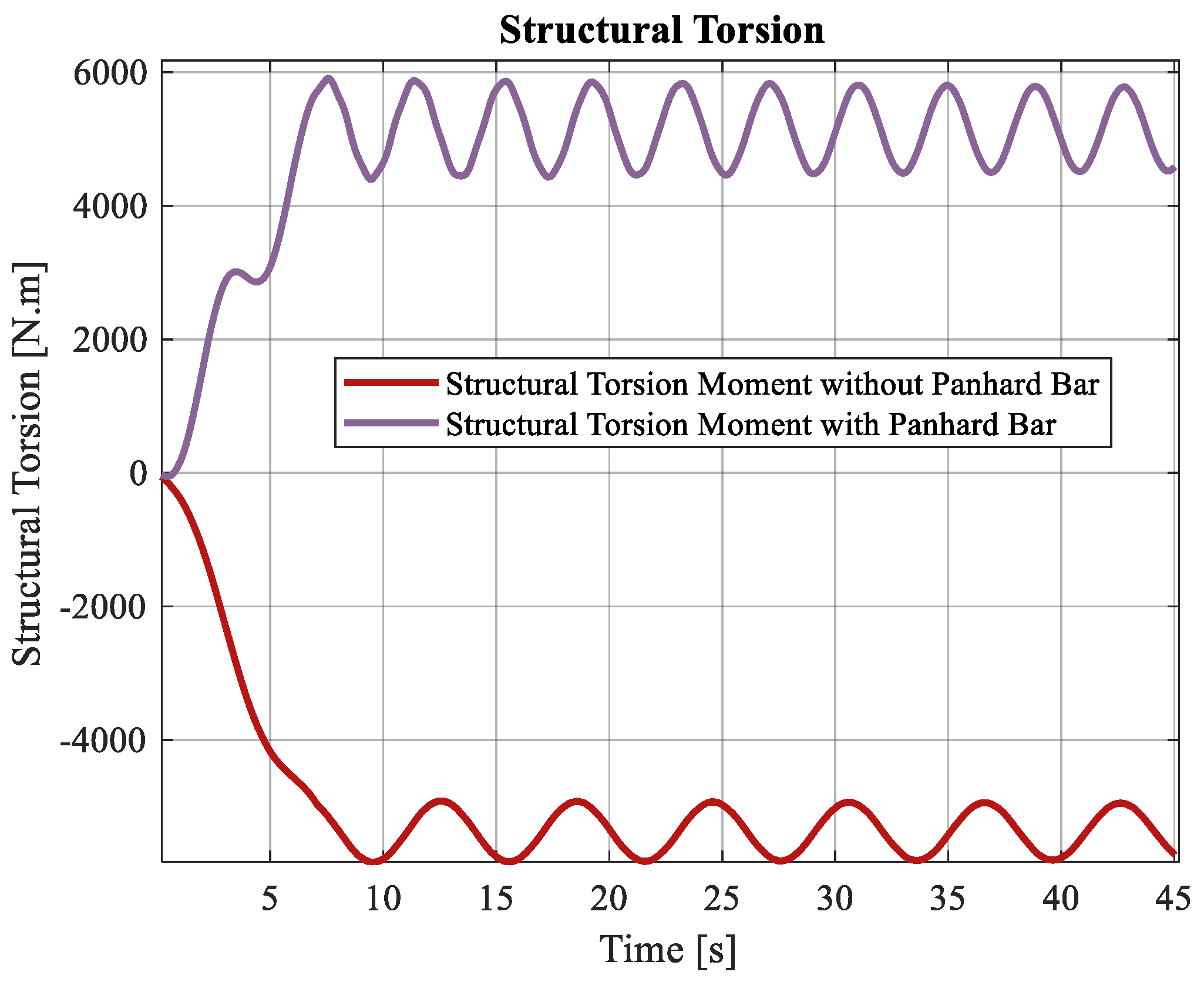
5.2. Panhard Bar Influence over the Structural Torsional Moment

As can be observed in the rotation angles comparison, there is an increment in the values in the system without a Panhard bar compared with the system with a Panhard bar. In fact, this tendency makes a change in the sense of the torsional moment produced along the structure of the bus, as can be seen in Figure 20.

The positive values of the structural moment present in the simulation with the Panhard bar show a better stability due to this moment acts in opposition to the vehicles rollover making the vehicle more stable; on the other hand, the absence of a Panhard bar produces a negative structural moment which contributes to an increased risk of rollover.

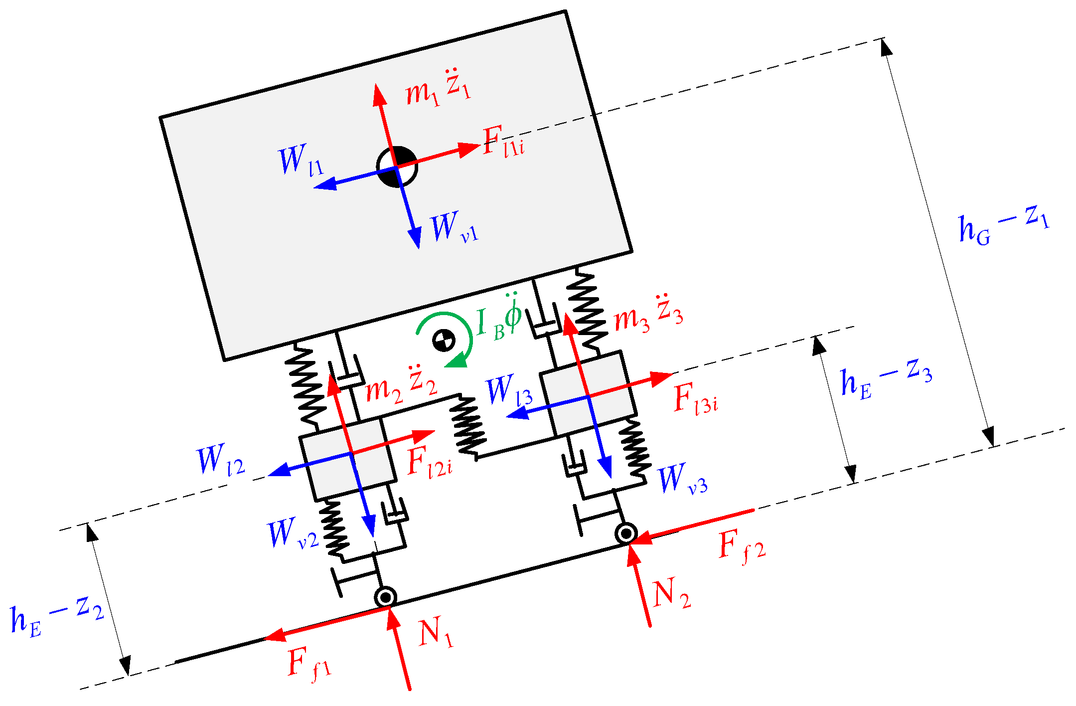
5.3. Vehicle Lateral Stability Analysis

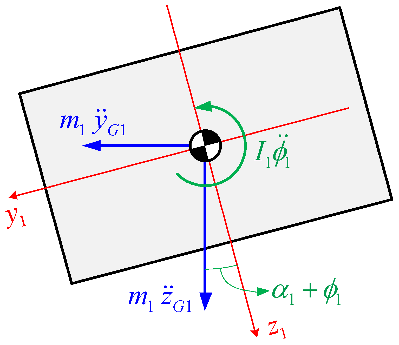
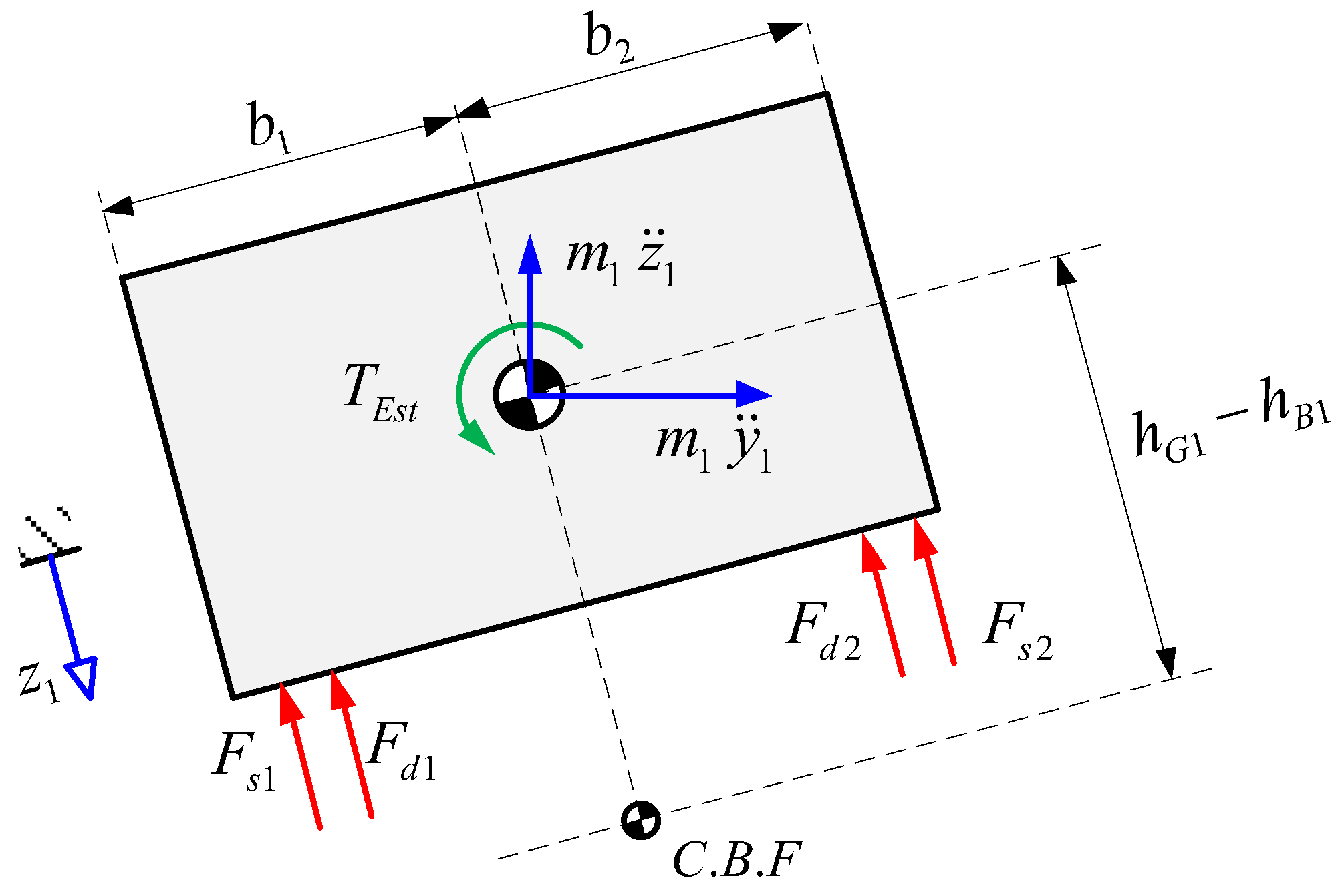
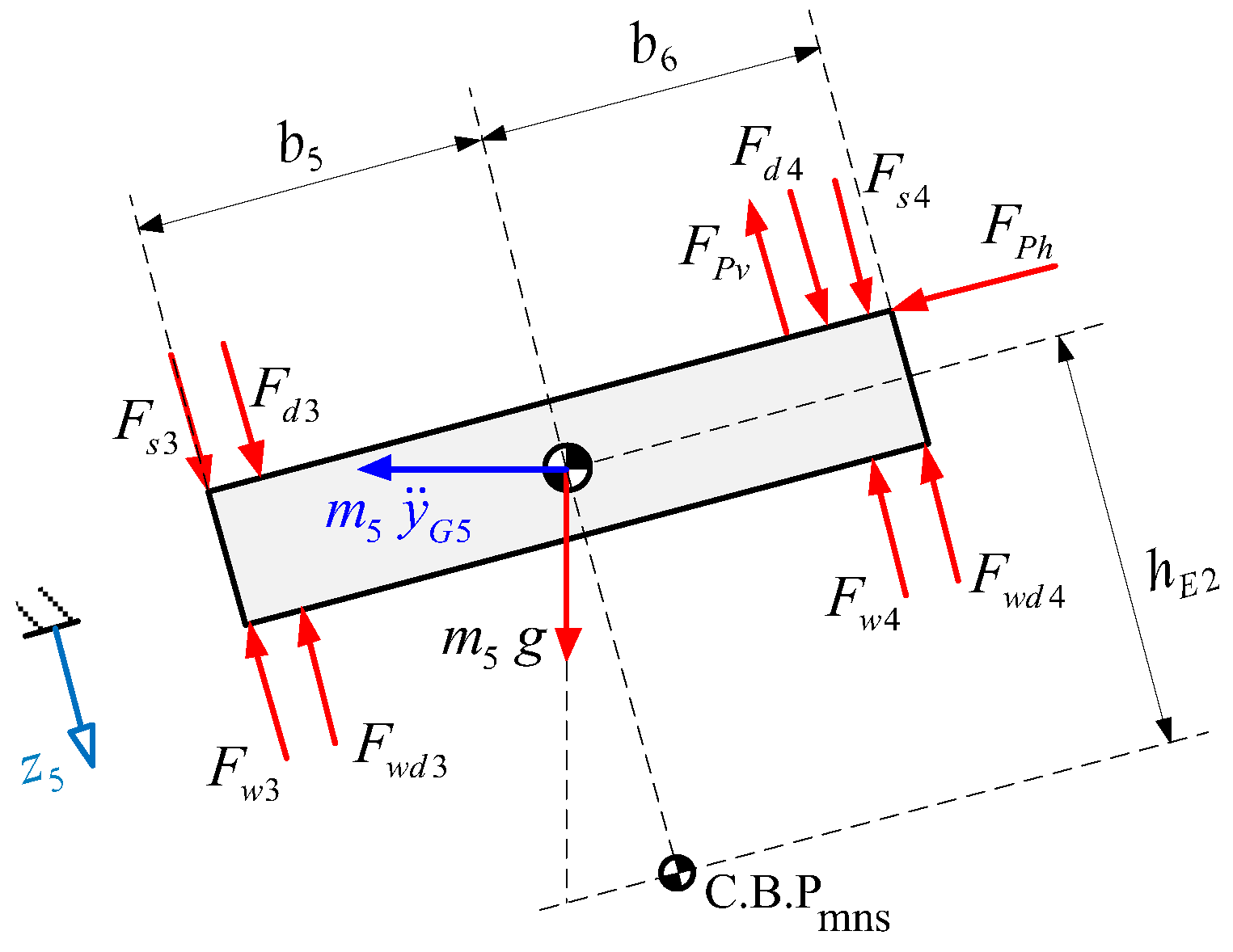
Although these results describe how the vehicle will behave, it does not show if the vehicle rolls over or slips; for that reason, it is necessary to handle the obtained results and the states derivatives in a new analysis that evaluates the normal and friction force on each tire. For this purpose, a new free body diagram is performed for the dynamic equilibrium in the front section (Figure 21).

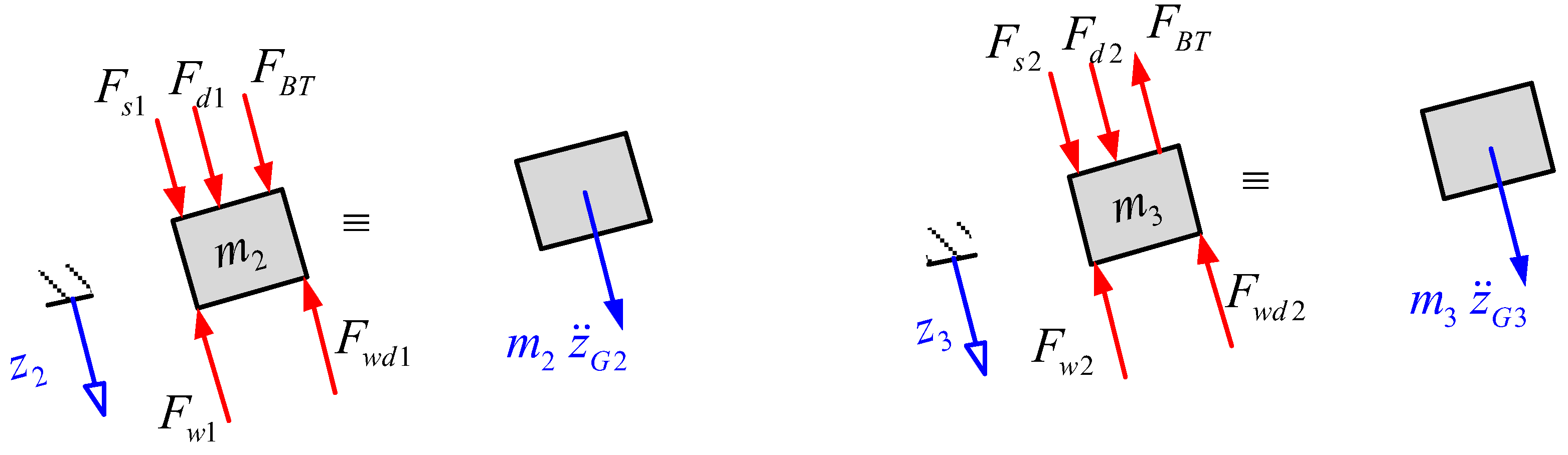
On the diagram shown, the inertial forces, which are obtained from the acceleration’s decomposition used for the motion equations, and weight of each body is already decomposed.

The inertia forces on the vertical direction are defined using the states derivatives, however, the lateral inertia forces and the weight decomposition are calculated as follow:

$$F_{l1i}=\frac{m_1 v^2}{{\rho }_1\left(t\right)}\cos \left[{\alpha }_1\left(t\right)+{\varphi }_1\left(t\right)\right]$$

(33)

$$F_{l2i}=\frac{m_2 v^2}{{\rho }_1\left(t\right)}\cos \left[{\alpha }_1\left(t\right)\right]$$

(34)

$$F_{l3i}=\frac{m_3 v^2}{{\rho }_1\left(t\right)}\cos \left[{\alpha }_1\left(t\right)\right]$$

(35)

Analyzing the equilibrium on the lateral direction:

$$F_{f1}+F_{f2}=F_{l1i}+F_{l2i}+F_{l3i}-W_{l1}-W_{l2}-W_{l3}$$

(36)

Furthermore, the inertial forces and torques required to be used into the state equations to calculate the normal forces at each tire. Analyzing the equilibrium taking moments from the left frontal wheel and factorizing $N_2$:

$$\left[\begin{array}{l}\left[W_{l2}-F_{l2i}\right]\left(h_{E1}-z_2\right)+\left[W_{l3}-F_{l3i}\right]\left(h_{E1}-z_3\right) -I_{1B} {\ddot{\varphi }}_1 \\ +\left[W_{l1}-F_{l1i}\right]\left(h_{G1}-z_1\right)+\left(m_1 {\ddot{z}}_1-W_{v1}\right)\left(B_{via}/2\right)+\left(m_3 {\ddot{z}}_3-W_{v3}\right)\left(a_{via}\right)\end{array}\right]/\left(B_t\right)$$

(37)

Analyzing the equilibrium on the vertical direction, $N_1$ is obtained:

$$N_1=W_{v1}+W_{v2}+W_{v3}-N_2-m_1 {\ddot{z}}_1-m_2 {\ddot{z}}_2-m_3 {\ddot{z}}_3$$

(38)

The magnitudes of the normal forces indicate if the vehicle rolls over or not when any normal force becomes zero. On the other hand, in the lateral direction there are two unknown variables, which are the friction force and just one equation, so that determines the value of each friction force becomes an unsolvable problem, therefore a new procedure to evaluate if the vehicle slips or not will be performed, using the value of both forces in a conditional way:

$$F_{f1}+F_{f2}\le F_{f1,\max }+F_{f2,\max }$$

(39)

In addition, it can be expressed as:

$$0\le N_1{\mu }_s+N_2{\mu }_s-F_{f1}-F_{f2}$$

(40)

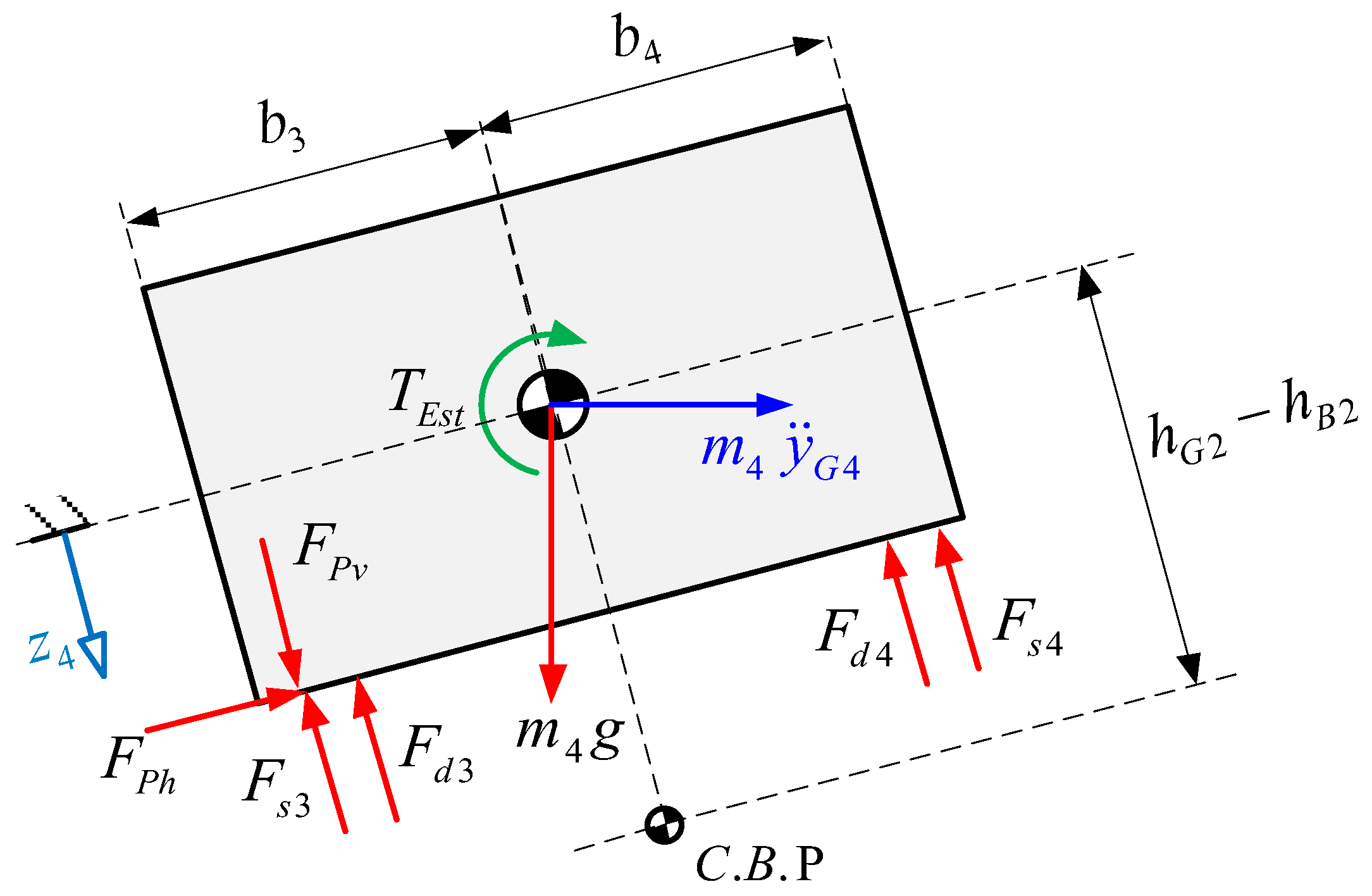
The maximum values of friction force will be determined using the so-called Coulomb’s dry friction approach. For that evaluation, it is assumed that both tires are not skidding, so the friction coefficient is the static friction coefficient. The conditional form establishes that when the value becomes negative it means that the vehicle is slipping. This analysis is also applied for the rear section, with a similar free body diagram (Figure 22).

The equations for the lateral inertia forces:

$$F_{l4i}=\frac{m_4 v^2}{{\rho }_2\left(t\right)} \cos \left[{\alpha }_2\left(t\right)+{\varphi }_4\left(t\right)+{\varphi }_5\left(t\right)\right]$$

(41)

$$F_{l5i}=\frac{m_5 v^2}{{\rho }_2\left(t\right)} \cos \left[{\alpha }_2\left(t\right)+{\varphi }_5\left(t\right)\right]$$

(42)

Analyzing the equilibrium on the lateral direction:

$$F_{f3}+F_{f4}=F_{l4i}+F_{l5i}-W_{l4}-W_{l5}$$

(43)

Similar to the front section, analyzing the equilibrium taking moments from the left wheel and factorizing $N_4$:

$$N_4=-\left[\begin{array}{l} \left[W_{l5}-F_{l5i}\right]\left(h_{E2}-z_5\right) -I_{B4} {\ddot{\varphi }}_4-I_{B5} {\ddot{\varphi }}_5+\left[W_{l4}-F_{l4i}\right]\left(h_{G2}-z_4\right)\\ +\left(m_4 {\ddot{z}}_4-W_{v4}\right)\left(B_{via}/2\right)+\left(m_5 {\ddot{z}}_5-W_{v5}\right)\left(B_t/2\right)\end{array}\right]/B_t$$

(44)

Analyzing the equilibrium on the vertical direction, $N_1$ is obtained:

$$N_3=W_{V4}+W_{V5}-N_4-m_4 {\ddot{z}}_4-m_5 {\ddot{z}}_5$$

(45)

Finally, the skidding condition is introduced for the rear section:

$$F_{f3}+F_{f4}\le F_{f3,\max }+F_{f4,\max }$$

(46)

In other terms:

$$0\le N_3{\mu }_s+N_4{\mu }_s-F_{f3}-F_{f4}$$

(47)

For the simulation, a parameter more is necessary:

${\mu }_k=0.4$—Static friction coefficient between the tire and path.

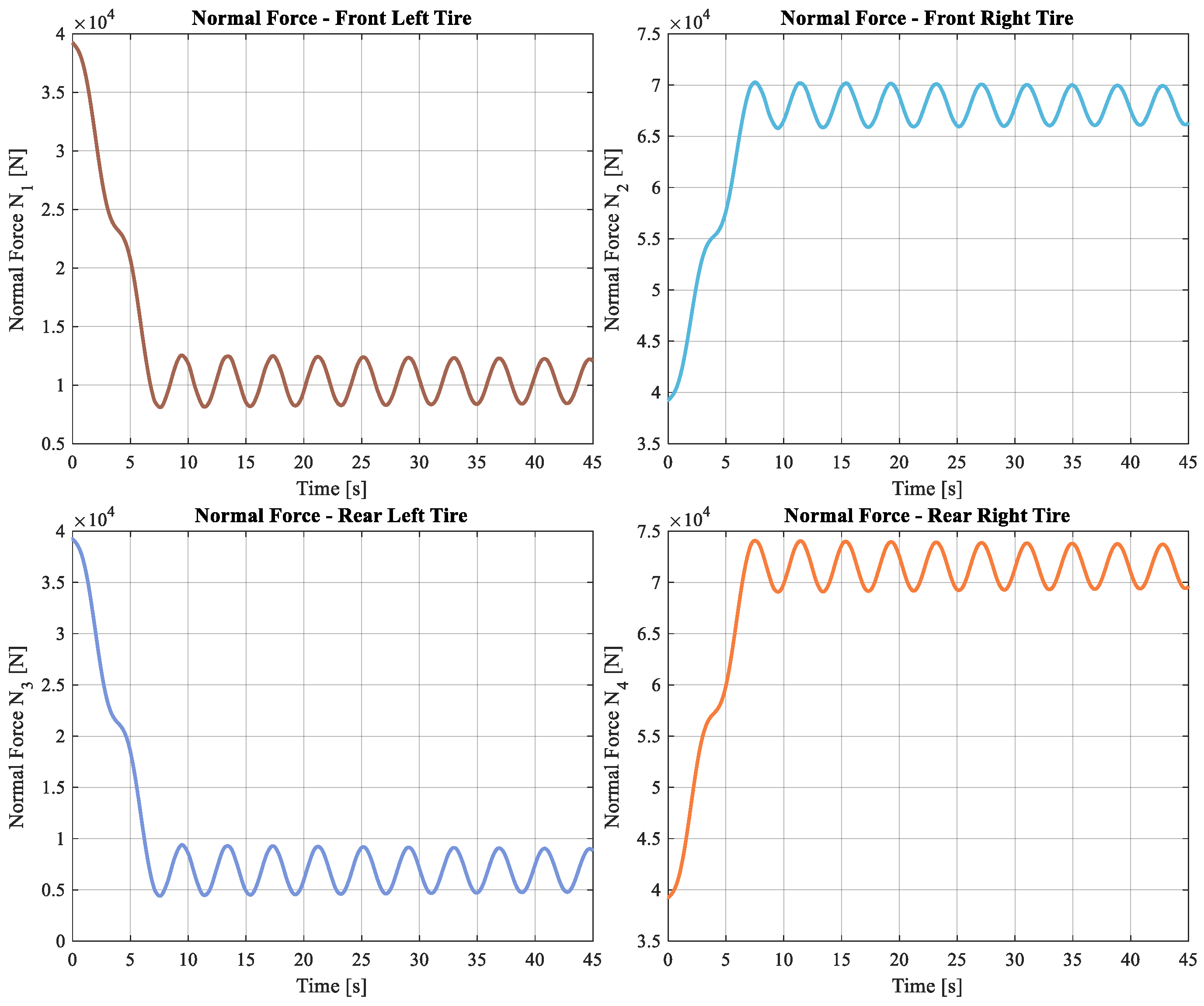
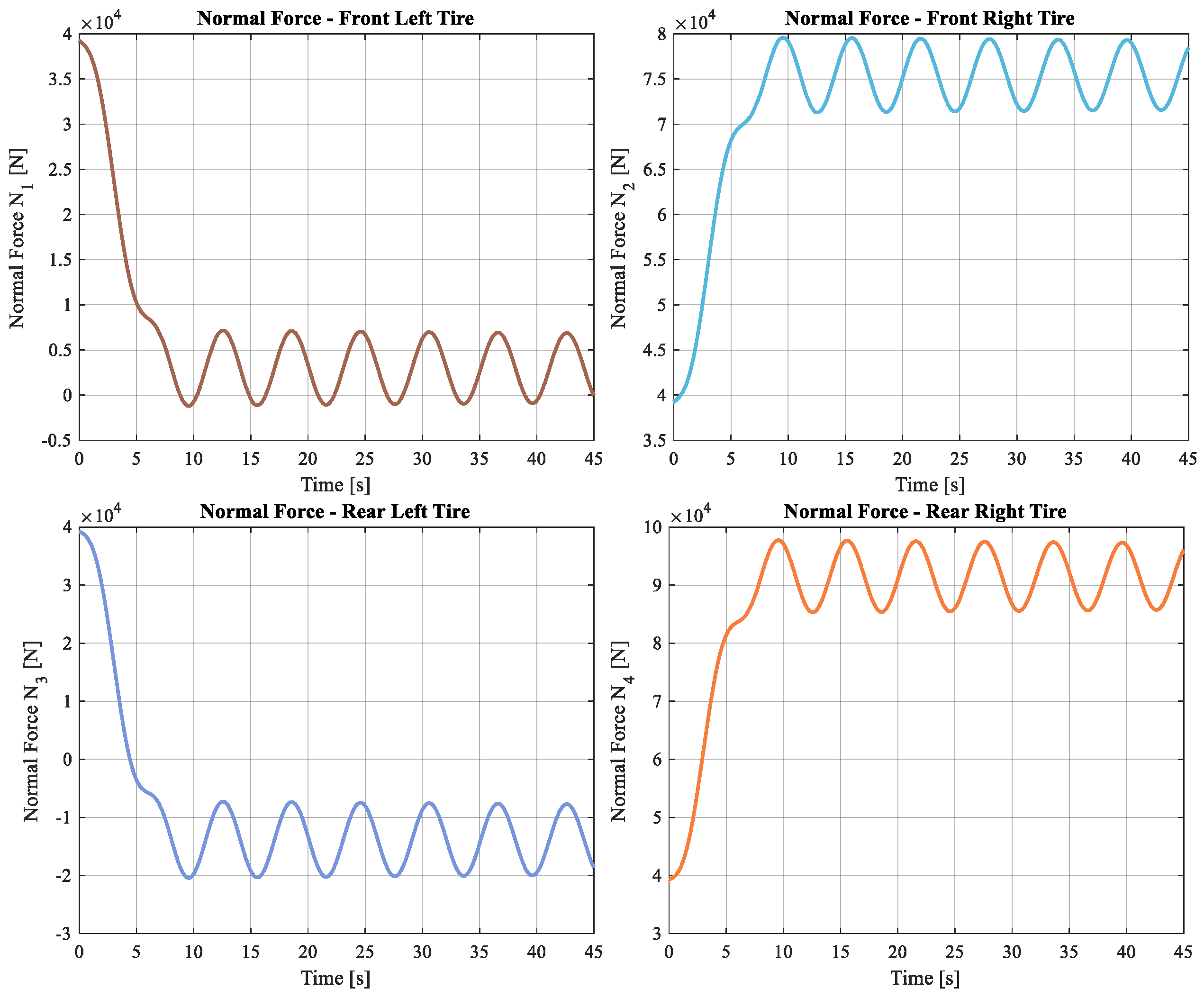
The results for the normal forces at each tire, while the bus is traveling over the simulation path, are shown on the following graphics (Figure 23).

About the friction force, the skidding condition shows the remaining friction force so that when it becomes negative the vehicle slips. Figure 24 shows the remaining friction force at each section, while the bus is traveling over the simulation:

A comparison of the normal force can be made using a model without a Panhard bar to analyze the effect of this element in the lateral stability. The normal force values of the bus without Panhard bar are presented in Figure 25.

From Figure 25, it is possible to observe that the normal force in the left side reach or even pass negative values, which implies that the vehicle loses adherence with the path. It demonstrates that the Panhard bar improves the adherence between the path and the tires.

6. Conclusions

A model of a bus is presented, elaborated by means of rigid multibody systems with which a virtual or mathematical model (system of ordinary differential equations) has been generated. This model allows the simulation of the lateral dynamics of a bus when it travels on a cambered curve.

Based on the proposed model, a simulation algorithm has been designed to analyze the dynamic behavior of a bus in transit on a cambered curve. This model is adjusted to realistic transport routes since it has been calculated and parameterized with curves of agreement (trajectories that connect a straight and circular trajectory in such a way that it starts with an infinite radius of curvature and ends in a constant radius of curvature) used in road design.

The modeling has been carried out in such a way that the total system representing the bus has been divided into two fundamental parts: the front part of the vehicle, which in turn contemplates several subsystems, such as the unsprung masses, the unsprung masses connected by a stability or sway bar, the flexible wheels, etc. In turn, the rear part has been modeled in an analogous way although, unlike the front part, in this one there is only one unsprung mass and a Panhard type bar is used to improve its vertical and lateral dynamic behavior.

Therefore, the model used to model the bus dynamic behavior integrates two modifiable sections that allow for testing some new models for the calculation of the stiffness of the suspension system or of the tires, etc. For this first approximation, the suspension system and tire stiffness as well as the damping of both bodies have been modeled as linear components. This is responsible for the quasi—linear correlation between the geometric parameters and the tendency shown in the results: the state variables increase as the geometric parameters of the trajectory increase and oscillate, trying to reach a steady state in time while the trajectory parameters are constant.

According to the comparison between the results with and without a Panhard bar, it can be stated that the Panhard bar has a stabilization function, which reduces the oscillations of each state variable. Additionally, the parameters which modify the Panhard bar stiffness can be treated as a control variable on an active suspension system.

From the effects on the rotation angles that the Panhard bar has, it is also possible to highlight that the presence of this element reduces the rotation angles of the mass linked to it, this improves the lateral stability of the vehicle, increasing the value of the normal forces between the tires and the road, as can be concluded by comparing Figure 23 and Figure 25.

The torsional structural stiffness is a parameter that must be considered when the stability of the vehicle is analyzed, as presented in Figure 20, where the direction of the structural moments affects the vehicle lateral stability.

Due to the weak effect of the non-linearities, some state variables have some disturbances which can be treated as noise.

References

1. Yang, S.; Chen, L.; Li, S. Dynamics of Vehicle-Road Coupled System; Springer: Berlin/Heidelberg, Germany, 2015. [Google Scholar]
2. Popp, K.; Schiehlen, W. Ground Vehicle Dynamics; Springer: Berlin/Heidelberg, Germany, 2010. [Google Scholar]
3. Rill, G.; Schaeffer, T. Grundlagen und Methodik der Mehrkörpersimulation—Vertieft in Matlab-Beispielen, Übungen und Anwendungen; Springer: Berlin/Heidelberg, Germany, 2014. [Google Scholar]
4. Schramm, D.; Hiller, M.; Bardini, R. Vehicle Dynamics—Modelling and Simulation; Springer: Berlin/Heidelberg, Germany, 2014. [Google Scholar]
5. Jeong, D.; Ko, G.; Choi, S.B. Estimation of sideslip angle and cornering stiffness of an articulated vehicle using a constrained lateral dynamics model. Mechatronics 2022, 85, 102810. [Google Scholar] [CrossRef]
6. Seyedi, M.; Jung, S.; Wekezer, J. A comprehensive assessment of bus rollover crashes: Integration of multibody dynamic and finite element simulation methods. Int. J. Crashworthiness 2020, 27, 273–288. [Google Scholar] [CrossRef]
7. Niculescu-Faida, O.-C.; Niculescu-Faida, A. Vehicle dynamics modeling during moving along a curved path. Mathematical model usage on studying the robust stability. UPB Sci. Bull. 2008, 4, 49–60. [Google Scholar]
8. Gauchia, A.; Olmeda, E.; Aparicio, F.; Díaz, V. Bus mathematical model of acceleration threshold limit estimation in lateral rollover test, Veh. Syst. Dyn. 2011, 49, 1695–1707. [Google Scholar] [CrossRef]
9. Gauchia, A.; Díaz, V.; Boada, M.J.L.; Olatunbosun, O.; Boada, B.L. Bus Structure Behaviour under Driving Manoeuvring and Evaluation of the Effect of an Active Roll System. Int. J. Veh. Struct. Syst. 2010, 2, 14–19. [Google Scholar] [CrossRef]
10. Eftekharzadeh, S.F.; Khodabakhshi, A. Safety evaluation of highway geometric design criteria in horizontal curves at downgrades. Int. J. Civ. Eng. 2014, 12, 326–332. [Google Scholar]
11. Yin, Y.; Wen, H.; Sun, L.; Hou, W. The Influence of Road Geometry on Vehicle Rollover and Skidding. Int. J. Environ. Res. Public Health 2020, 17, 1648. [Google Scholar] [CrossRef] [PubMed]
12. Wang, B.; Hallmark, S.; Savolainen, P.; Dong, J. Crashes and near-crashes on horizontal curves along rural two-lane highways: Analysis of naturalistic driving data. J. Saf. Res. 2017, 63, 163–169. [Google Scholar] [CrossRef] [PubMed]
13. Geedipally, S.R.; Pratt, M.P.; Lord, D. Effects of geometry and pavement friction on horizontal curve crash frequency. J. Transp. Saf. Secur. 2019, 11, 167–188. [Google Scholar] [CrossRef]
14. Bogenreif, C.; Souleyrette, R.R.; Hans, Z. Identifying and measuring horizontal curves and related effects on highway safety. J. Transp. Saf. Secur. 2012, 4, 179–192. [Google Scholar] [CrossRef]
15. Abdollahzadeh Nasiri, A.S.; Rahmani, O.; Abdi Kordani, A.; Karballaeezadeh, N.; Mosavi, A. Evaluation of Safety in Horizontal Curves of Roads Using a Multi-Body Dynamic Simulation Process. Int. J. Environ. Res. Public Health 2020, 17, 5975. [Google Scholar] [CrossRef] [PubMed]
16. Xu, J.; Xin, T.; Gao, C.; Sun, Z. Study on the Maximum Safe Instantaneous Input of the Steering Wheel against Rollover for Trucks on Horizontal Curves. Int. J. Environ. Res. Public Health 2022, 19, 2025. [Google Scholar] [CrossRef] [PubMed]
17. Yin, Q.; Stiharu, I.; Rakheja, S. Kinetostatic analysis of a beam-axle suspension with Panhard rod restraining linkage. Int. J. Veh. Des. 1998, 19, 108–123. [Google Scholar]
18. Mayr, S.; Wagner, W. Development of a front axle suspension for special purpose tractors. In Proceedings of the Conference: Agricultural Engineering 2004, Dresden, Germany, 7–8 October 2004. [Google Scholar]
19. Sonsino, C.M.; Streicher, M. Optimization of cast iron safety components of commercial vehicles by material selection and geometry under consideration of service loadings. Mater. Test.-Mater. Compon. Technol. Appl. 2009, 51, 428–436. [Google Scholar]
20. Torbic, D.J.; O’Laughlin, M.K.; Harwood, D.W.; Bauer, K.M.; Bokenkroger, C.D.; Lucas, L.M.; Ronchetto, J.R.; Brennan, S.; Donnell, E.; Brown, A.; et al. NCHRP 774 Report: Superelevation Criteria for Sharp Horizontal Curves on Steep Grades; The National Academie Press: Washington, DC, USA, 2014. [Google Scholar]
21. Esveld, C. Modern Railway Track; Delft University, MRT—Productions: Zaltbommel, The Netherlands, 2001. [Google Scholar]
22. Rajamani, R. Vehicle Dynamics and Control; Mechanical Engineering Series; Springer: Berlin/Heidelberg, Germany, 2012. [Google Scholar]
23. Aparicio, F.; Vera, C.; Díaz, V. Teoría de los Vehículos Automóviles; Sección de Publicaciones, ETSII, Universidad Politécnica de Madrid: Madrid, Spain, 1995. [Google Scholar]
24. Mustafa Siddiqui, O. Dynamic Analysis of a Modern Urban Bus for Assessment of Ride Quality and Dynamic Wheel Loads. Master’s Thesis, Concordia University, Montreal, QC, Canada, 2000. [Google Scholar]
Figure 1. Path’s geometric parameters.
Mathematics 10 03081 g001
Figure 2. Force Schema for a vehicle traveling over a curved path.
Mathematics 10 03081 g002
Figure 3. Clothoid curve.
Mathematics 10 03081 g003
Figure 4. Simulation path—plane view.
Mathematics 10 03081 g004
Figure 5. (a) Curvature radius vs. time and (b) camber angle vs. time for simulation.
Mathematics 10 03081 g005
Figure 6. Bus front section—mathematical model.
Mathematics 10 03081 g006
Figure 7. Bus rear section—mathematical model.
Mathematics 10 03081 g007
Figure 8. Complete bus model.
Mathematics 10 03081 g008
Figure 9. Acceleration decomposition.
Mathematics 10 03081 g009
Figure 10. Front cabin’s free body diagram for dynamic equilibrium.
Mathematics 10 03081 g010
Figure 11. Unsprung frontal masses free body diagram.
Mathematics 10 03081 g011
Figure 12. Free body diagram—sway bar.
Mathematics 10 03081 g012
Figure 13. Rear cabin’s free body diagram for dynamic equilibrium.
Mathematics 10 03081 g013
Figure 14. Rear unsprung mass free body diagram for dynamic equilibrium.
Mathematics 10 03081 g014
Figure 15. Rear masses displacements at the ends connected to the Panhard Bar.
Mathematics 10 03081 g015
Figure 16. Panhard Bar vertical displacement.
Mathematics 10 03081 g016
Figure 17. Simulation results—Displacement and rotation angles.
Mathematics 10 03081 g017
Figure 18. Panhard bar—force and inclination angle.
Mathematics 10 03081 g018
Figure 19. Simulation results without Panhard bar—displacement and rotation angles.
Mathematics 10 03081 g019
Figure 20. Structural Torsion with and without Panhard bar.
Mathematics 10 03081 g020
Figure 21. Free Body Diagram for front section dynamic equilibrium.
Mathematics 10 03081 g021
Figure 22. Free Body Diagram for rear section dynamic equilibrium.
Mathematics 10 03081 g022
Figure 23. Normal forces on each tire considering Panhard bar.
Mathematics 10 03081 g023
Figure 24. Remaining friction force at each section.
Mathematics 10 03081 g024
Figure 25. Normal forces on each tire without Panhard bar.
Mathematics 10 03081 g025