Abstract
This paper describes a comparison of three types of feature sets. The feature sets were intended to classify 13 faults in a centrifugal pump (CP) and 17 valve faults in a reciprocating compressor (RC). The first set comprised 14 non-linear entropy-based features, the second comprised 15 information-based entropy features, and the third comprised 12 statistical features. The classification was performed using random forest (RF) models and support vector machines (SVM). The experimental work showed that the combination of information-based features with non-linear entropy-based features provides a statistically significant accuracy higher than the accuracy provided by the Statistical Features set. Results for classifying the 13 conditions in the CP using non-linear entropy features showed accuracies of up to 99.50%. The same feature set provided a classification accuracy of 97.50% for the classification of the 17 conditions in the RC.
Keywords:
approximate entropy; non-linear systems; phase space reconstruction; fault classification; random forest; support vector machines MSC:
28D20
1. Introduction
In industrial applications, centrifugal pumps are equipment for transferring energy to fluids to enable pipeline transportation. Similarly, reciprocating compressors are essential in petrochemical plants and refineries for gas and other fluid transportation. Reliable functioning of these types of equipment is essential in industry to avoid unexpected halting of processes and economic losses. Consequently, several condition monitoring (CM) methods have been proposed for diagnosing faults in centrifugal pumps and reciprocating compressors [1,2,3].
The CM methods are based on sensing several variables from the target equipment, such as electrical current, vibration, sound, temperature, or acoustic emission. Some of the most common variables are vibration signals recorded using accelerometer sensors. Such a set of signals is processed for extracting features useful for fault detection and classification. Traditional techniques for vibration signal analysis are divided into time, frequency, and time-frequency methods. In general, signal processing techniques assume that signals represent linear systems that comply with the stationary and periodicity condition. Unfortunately, this assumption is not always met. In particular, in most rotatory machines, the vibration signals represent a non-linear system [4]. These constraints can be efficiently handled using chaos theory and non-linear dynamics techniques.
In this work, we propose to use the approximate entropy (AppEn) [5,6] and variants, such as the sample entropy (SampEn) [7,8] and fuzzy entropy (FuzzyEn) [9,10] for fault classification. The emphasis of this research is feature extraction. The classification stage can be performed using either classical or deep learning-based classifiers. However, as the feature extraction is computationally expensive, selecting deep learning models would impose an unnecessary cost. In consequence, we have selected two efficient classical models corresponding to RF and the multi-class SVM [11,12]. The original contributions of this research are the following:
- Extraction of a non-linear entropy-based feature set that provides high classification accuracy using RF and SVM models. The accuracy attained by the SVM model trained with the non-linear Entropy Features set was higher than the accuracy attained by a CNN model trained with 2D spectrogram images for both the CP and the RC.
- Detailed comparison of three feature sets useful for classifying a large number of faults in a CP and an RC. These are the non-linear Entropy Features, the Information Entropy, and the Statistical Features sets. The first set is composed of the approximate entropy and several variants, and the second set is composed of the combination of the wavelet packet transform (WPT)-based features and the power spectrum entropy (PSE)-based features. Finally, the third set is composed of classical time series statistical features.
- The non-linear Entropy Features set and the All Features set corresponding to the fusion of the three feature sets when compared provided a classification accuracy of up to 99.59% for the CP and up to 97.90% for the RC. For the CP, 13 different conditions were classified, and 17 valve conditions were classified for the RC.
The paper is organized as follows: in Section 3 the theoretical background is presented. In Section 4, the test bed for acquiring the vibration signals from the CP and RP is presented. In Section 5 and Section 6, the methodology for extraction of the different sets of features is described. The methodology for classifying faults using RF and SVM models based on the extracted features is presented in Section 7. The results are described in Section 8, and finally, the conclusion and future work are presented in Section 10.
2. Related Research
The related research is discussed in the following subsections. A compendium with several publications is presented in Table A1 in terms of their main features. A brief revision concerning these publications is presented in Section 2.1, Section 2.2 and Section 2.3.
2.1. Rotating Machinery
Although non-linear entropy methods have been used for classifying a small set of faults in centrifugal pumps and reciprocating compressors, attaining high accuracy, their application to other rotatory machines (RM) has also been reported. Research concerning the correlation dimension (CD) is presented in [13]. The approach analyzes the vibration signal measured from a roller element bearing. Results allow them to conclude that CD features show significant statistical differences between a roller element close to failure and a new one. The largest Lyapunov exponent (LLE) [14] has been used to show that faults in non-linear rotatory systems can be detected early when the onset of the fault occurs. This feature evolves as the fault progresses. The research reported in [4] combines the CD, the approximate entropy, the LLE, and visualization of the phase space for detecting damage in bearings and gearboxes. In [15], a method for classifying seven different conditions in roller bearings and ten types of conditions on a gearbox is reported. The approach is based on features extraction from the Poincaré plot and their classification using SVM. The accuracy attained was 100% for the roller bearings and 99.3% for the gearbox dataset. A combination of the spectral graph wavelet transform (SGWT) with detrended fluctuation analysis (DFA) was used for denoising the vibration signals in RM [16]. The first stage is converting the vibration signal into a graph signal. The SGWT is used for decomposing the graph signal into scaling function coefficients and spectral graph wavelet coefficients. DFA is used for selecting the level of decomposition of SGWT. A bi-dimensional representation of vibration signals denoted as the complexity-entropy causality plane (CECP) useful for fault classification in RM is reported in [17]. This 2D representation was obtained with the normalized permutation entropy and the Jensen–Shannon complexity of time series. The authors showed the utility of this representation for improving the classification accuracy of faults in roller bearing and gear applications using SVM models. A review of entropy algorithms and its variants in RM is reported in [18,19]. The reviews briefly introduced several entropy methods and their application in fault detection in RM.
2.2. Reciprocating Compressor
An application of faults diagnosis in an RC using multi-scale entropy is reported in [20]. After performing the signals’ local mean decomposition (LMD), vibration signals’ multi-scale entropy (MSE) features were calculated. Four conditions were classified using SVM, obtaining a classification accuracy of 95.0%. In a previous study [2], a method for feature extraction from vibration signals recorded from an RC is proposed to classify 13 different conditions of combined faults in valves and roller bearings. The feature extraction method was based on symbolic dynamics and complex correlation measures. The extracted features were used for fault classification using several machine learning models, attaining accuracy of up to 99%. Research concerning the fault diagnosis and severity of valve leakage in an RC is reported in [21]. The diagnosis was performed using features extracted from the diagram using principal component analysis (PCA) and linear discriminant analysis (LDA). The method showed that the diagram’s features help classify two types of faults with several levels of severity, attaining classification accuracies of up to 99.62%. The research reported in [22] concerns the classification of faults based on images representing the diagram. A set of features is extracted from the images for classifying eight health conditions in valves, piston rings, and valve springs. Accuracies of up to 97.9% were obtained using artificial neural network (ANN) models. Research reported in [23] combines the binary moth flame optimization (BMFO) algorithm with the K-nearest neighbor (KNN) algorithm for classifying three types of valve faults in an RC, attaining accuracies higher than 99%. Research concerning convolutional neural networks (CNNs) for classifying faults in an RC is reported in [24]. The vibration signal was re-arranged into a 2D format by bringing its time samples into lines that moved 45 degrees counterclockwise to reinforce their features. This array was fed to the CNN that incorporated the attention mechanism through squeeze-and-excitation (SE) modules. The maximum accuracy attained was 99.4%. Classification of four different valve conditions using 1D and 2D CNNs is reported in [25]. The classification was performed using vibration signals in the case of the 1D CNN and considering the fusion of seven channels (four channels with vibration signals and three channels with pressure) in the case of 2D CNN. The classification was performed for different SNR values of the signals, and the highest classification accuracy was 100% for signals with more than 20 dB of SNR. The CNN used has a complex architecture.
2.3. Centrifugal Pump
The permutation entropy features are used in a fault detection method reported in [26]. The method was applied to hydraulic pump (HYP) fault detection. The vibration signal was processed using resonance-based sparse signal decomposition (RSDD). A Multi-scale hierarchical amplitude-aware permutation entropy (MHAAPE) method was applied for feature extraction. Four fault conditions were classified using a probabilistic neural network, SVM models, and extreme learning machines (ELM). The approach attained an accuracy of up to 100%. A method for faults diagnosis in a CP is reported in [27]. The method is based on applying complementary ensemble empirical mode decomposition (CEEMD) to vibration signals. The decomposed signals or intrinsic mode functions are processed for extracting the SampEn. The set of features is used for classification; RF attained classification accuracies of 94.58% for classifying five conditions. A feature extraction approach from vibration signals is reported [28] to classify faults in a CP. The discriminant feature extraction method includes three stages. The first stage is the healthy baseline signal selection. The second stage is devoted to cross-correlating the healthy baseline signals with the vibration signals of different fault classes. A set of features is extracted from the resultant correlation sequence. In the third stage, time, frequency, and time–frequency domain raw hybrid features are extracted from baseline signal and vibration signals from faulty classes. A new set of discriminant features is composed of the correlation coefficient between raw hybrid feature pools. The combination of all extracted features is fed to an SVM model for classification. The method is used to classify four conditions in a CP, attaining accuracy of up to 98.4%. A method for fault classification in a CP based on vibration signals is reported in [29]. A feature extraction pre-processing is used to obtain a time-frequency representation using the continuous wavelet transform (CWT). The CWT is converted to gray images fed to a CNN model with an adaptive learning rate. Accuracies of 100% are obtained for classifying four different fault conditions. A fault classification method of a multi-stage CP reported in [30] starts by selecting the fault-specific frequency band and continues by extracting statistical features in time, frequency, and wavelet domains from this band. The next step is to select a low dimensional features vector using the informative ratio PCA. The classification of four conditions in a multi-stage CP using KNN models. The accuracy attained was 100%. Fault detection and classification for water pump bearings based on features extracted from the instantaneous power spectrum is reported in [31]. The instantaneous power spectrum (IPS) was obtained with the voltage and current measured, and several features were extracted from the IPS for classifying three different conditions at different load levels. The classification was performed using an extreme gradient boosting (XBG) model [32]. The application of CNN for classifying faults in a CP based on acoustic images is reported in [33]. In this application, the sound signals were acquired from a CP test rig where five different health conditions were implemented. The sound signals were converted into acoustic images using the analytical wavelet transform (AWT). The acoustic images were fed to the CNN for classification. The attained accuracy was 100%.
2.4. Anomaly Detection
Anomaly detection corresponds to identifying events within a stream of data features that deviate significantly from most available data. Anomaly detection has applications in many fields. This topic is relevant because the non-linear entropy-based features have found applications in the context of anomaly detection. Examples of applications have been reported in [34,35,36,37,38,39]. Several authors have proposed anomaly detection applications centered around deep learning. Approaches such as CNN, autoencoders, and generative adversarial networks [40,41,42] can be used for anomaly detection implementation. Research concerning anomaly detection in RM is active. An example is reported in [41] for anomaly detection in gearboxes where a prototype selection algorithm is used for improving the training of the feature extractor implemented with a CNN. The research reported in [40] uses an autoencoder for learning to model the healthy state of the rotating machine. Such a learning process is performed using vibration signals representing the healthy state. The anomaly is detected using a threshold-based approach to the reconstruction error of data acquired from an unknown state. The algorithm was validated with the IMS bearings dataset. Other recent applications of anomaly detection in RM and also in other fields are reported in [41,43,44,45,46].
3. Theoretical Background
3.1. Phase Space Reconstruction
The phase space reconstruction method is based on the embedding theorem of Taken, reported in [47]. The theorem postulates that we can recover the equivalent dynamics of a non-linear system by using time delays from a recorded time-domain signal. The approximate dynamics correspond to a 1D projection of the system trajectory. The theorem is mainly applied to univariate time series [47]; however, the multivariate version has also been reported in [48]. In this research, we are mainly concerned with univariate embedding.
The average mutual information (AMI) enables the selection of the time delay or lag denoted [49]. The AMI is plotted versus . According to [50], the selection of could be the location of the first local minimum of the AMI. The system’s embedding dimension, denoted as m, could be selected by applying the false nearest neighbors (FNN) method, as reported in [51].
3.2. Approximate Entropy
Given a signal denoted including N samples, the AppEn [5,6] measures the regularity of the time-series. The time-series regularity and dynamics are estimated considering a higher order dimensional space generated by a series of vectors represented by time-delayed components of . The AppEn is calculated for a time-series of length N, representing a system with embedding dimension m, lag , and a distance threshold between vectors denoted r. In general, the calculation of the AppEn should consider a window of the signal with length N large enough to reduce the bias in the estimation [6]. However, a limitation is that extending N can significantly increase the computational cost. AppEn has the advantage of being robust to noise and outliers (see [52] for a detailed review concerning entropy calculation methods).
3.3. Sample Entropy
The SampEn is obtained through modification of the AppEn algorithm [7]. The modification consists of the elimination of self-matches in the evaluation of the distance between lagged vectors. The SampEn avoids the bias introduced in ApEn by considering self-matches. The resultant features are more consistent and unbiased, even when their calculation uses short-length signal windows. In addition, the calculation of SampEn is more straightforward than the calculation of AppEn.
3.4. Fuzzy Entropy
The FuzzyEn measure [10] is a variant of the AppEn that modifies the function used for estimating the similarity between lagged vectors. The algorithm’s modification is based on changing the Heaviside function for a fuzzy exponential membership function. The calculation of FuzzyEn also incorporates the modifications introduced for the calculation of the SampEn.
3.5. Shannon Entropy and Other Measures of Signal Complexity
The entropy measure enables quantification of the complexity of a non-linear dynamical system. The Shannon entropy (ShannEn) quantifies the amount of information in a system. In addition, the conditional entropy quantifies the rate of information generation [53,54]. Other entropy measures, such as corrected conditional entropy, can be estimated based on these measures. A detailed review of ShannEn estimation is presented in [55].
3.6. Permutation Entropy
The permutation entropy (PermEn) is based in partitions [56]. When the time series takes many values, their range can be replaced with a symbol sequence . This is done by defining the partition of the signal range . Based on this partition, the symbol is defined if is in . The PermEn is calculated for different embedding dimensions m; however, for practical purposes . Denote by the permutation of order m with probability given as ; then, the PermEn is calculated using Equation (1):
This research used the method reported in [57] for computing the PermEn. The method is based on pre-calculating values for successive ordinal patterns of order m. This approach allows the calculation of PermEn in large time series using overlapped successive time windows.
3.7. The Correlation Dimension
The system’s phase space enables the calculation of complexity [58] that is quantified using several non-linear features such as SampEn. In addition, another feature is the CD which quantifies the number of independent lagged vectors required for defining a system [59]. Details concerning the estimation of this feature are presented in [60].
3.8. Detrended Fluctuation Analysis
The fractal scaling properties quantified in short intervals of time-series [61] can be performed using DFA. This approach enables quantitative analysis of non-stationary time-series [62]. Their calculation requires performing the integration of the signal, subdividing such a signal into several segments, finding the trend of the signal using least-square approximations, and calculating the average fluctuation of the signal around the trend. Details of the estimation of this feature are presented in [63].
3.9. Largest Lyapunov Exponent
The Lyapunov exponent quantifies the relative motion of trajectories in the phase-space of a system [64]. Its value allows for determining if a signal is chaotic or periodic. A system can be represented by several Lyapunov exponents determined by the embedded dimension. However, the largest one, denoted , is typically used. There are several algorithms for calculating the Lyapunov exponent [65]. The method proposed by Rosenstein et al. [66] was implemented in this research.
3.10. Information Entropy and Chaotic Time Series
Information entropy was proposed by Claude Shannon [67] in the context of theoretical communication modeling. A collection of messages sent through a communication channel can be considered as independent random events with probabilities , where . Information entropy is defined as:
The entropy concept is also used in classical thermodynamics in the context of heat transfer [68]. Gibbs and Boltzmann attained a definition of entropy with an expression similar to Equation (2) [69]. When dealing with discrete-time signals represented as a vector, the entropy concept has also been applied to select the best basis for orthogonal wavelet packets [70]. The authors showed that the assumption that the Karhunen–Loeve basis is the best, even for a single vector which enables the calculation of several entropy features. Consider the time-series where the vector can be arranged in decreasing order such that for large i. Then, . Without loss of generality, the time-series can be normalized so . The following features can be estimated: the log energy entropy, the Shannon information entropy, the norm entropy, the threshold entropy, and the “sure” entropy.
3.10.1. Tsallis and Rényi Entropy
In the context of systems with complex behavior (including, for instance, chaotic motion or fractal evolution), Tsallis [71] has proposed an alternative definition of entropy as:
where K is a positive constant and q denotes any real number. Tsallis showed that when , tends to the classical Boltzmann–Gibbs–Shannon entropy represented by Equation (2). Similarly, q is used in the Rényi entropy [72] to amplify probabilities as:
Both entropies are parameterized representations of the Boltzmann–Gibbs–Shannon entropy, where one parameter is used for weighting the probabilities to evaluate different fractal properties of the system.
3.10.2. Power Spectral Entropy
The complexity can also be quantified using the power spectral density of time-series [73,74]. This feature has been used for fault detection in gearboxes and roller bearings. The normalized power spectral density of the time series is denoted , and it can be expressed as:
This equation enables the calculation of the power spectral entropy (PSE) as:
The PSE is calculated for each time frame and is a vector denoted as . When the signal has high complexity, the spectrum of the time series tends to be uniform, and the PSE is high. In contrast, when the spectrum has a narrow peak, the PSE feature is lower, and the signal is less complex.
3.11. Machine Learning Techniques
3.11.1. Random Forest
The RF algorithm is a machine learning algorithm that combines a set of weak learners using ensemble methods to attain a high-quality classification or regression model [75]. The most common weak learners in the RF model are tree-type classifiers used for growing forests of randomized trees using bootstraps resampling techniques [76].
3.11.2. Support Vector Machines
The machine learning model proposed by Vapnik [77] is the SVM. In its more basic form, the SVM is used for solving problems of binary classification where the data in each of the classes can be separated using a hyperplane that can be constructed based on the support vectors, as detailed in [78]. In practical applications, the SVM incorporates higher-dimensional transformation represented as kernels for transforming the feature space to increase class separability. Similarly, multi-class support vector machines are also available, as reported in [11].
4. Experimental Test-Bed
In this research, two different vibration signal datasets were considered. The first was acquired from a CP and the second from an RC.
4.1. Centrifugal Pump Test-Bed
In this research, a multi-stage vertical CP is considered. The CP model 3SV10GE4F20 was a 2 HP pump operated at 3500 rpm. The pump had ten stages for a nominal flow of 15 GPM. The vibration signals were recorded using model 603C01 accelerometers. The module NI 9234 connected to a laptop computer was used to acquire the vibration signal using a sampling frequency of 50 kHz. The physical description and locations of sensors are shown in Figure 1. The signal acquisition was performed under controlled operating conditions concerning the room temperature, relative humidity, and environmental noise.
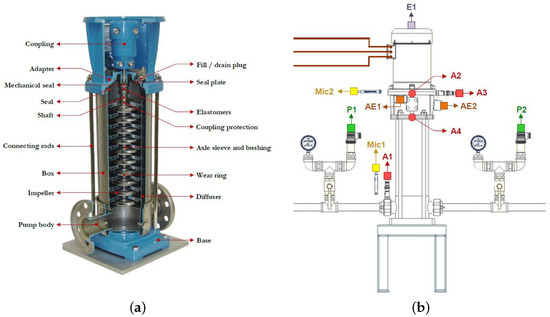
Figure 1.
CP and sensors. (a) Multi-stage vertical CP. (b) Locations of sensors. The vibration signals were recorded using A1, A2, A3, and A4 accelerometers.
Six experimental conditions were considered related to the discharge pressure. The conditions are denoted as with i ranging from 1 to 6. The pressure started at 5.5 bar, increasing by 1 bar for each condition. corresponds to a discharge pressure of 5.5 bar.
4.1.1. Faults of the CP
A set of 13 impeller faults were configured in the CP. One condition corresponded to a CP where all stages were healthy. Three conditions involved pitting at the entrance of the impeller blades (PEB), three conditions involved pitting at the output of the impeller blades (POB), three conditions involved impeller channel blockade (ICB), and finally, three conditions involved an imbalanced impeller (IB). The pitting and impeller blockade can affect several stages of a pump with different levels of severity. For instance, in fault P3, the severity level for stage 6 was 1, and the severity increased with the stage number, and it was 5 for stage 10. The pitting severity levels were attained by changing the number and diameter of holes in the blades. The ICB severity levels were attained by varying the percent of blocked channels in the impeller. The impeller imbalance severity was obtained by increasing the surface of the cut portion of the impeller front cover. Table 1 presents the list of configured faults.

Table 1.
Faults conditions in the CP.
4.1.2. CP Vibration Signal Dataset
The vibration signal acquisition was performed by maintaining the environmental condition within a controlled range. The motor rotation was set to 3600 rpm. A pressure condition was set, and the vibration signal was acquired during 10 s. Ten repetitions were performed for each of the faults conditions P1 to P13. Consequently, 60 vibration signals were recorded for each condition. A total of 780 vibration signals are included in the dataset, including all fault conditions.
4.2. Reciprocating Compressor Test-Bed
The RC test bed is centered around a compressor model EGB-250 with two stages. The compressor is driven by an induction motor with a power of 5.5 HP that operates at 3470 rpm.
A detailed description of the test bed is described in [2]. The test bed incorporates several accelerometer sensors for acquiring the vibration signals. The accelerometers are denoted as A1, A2, A3, and A4 and were located as shown in Figure 2. Module NI9234 was used to acquire the vibration signals from model 603C01 accelerometers. The sampling frequency was 50 kHz. The acquired vibration signals were transferred to a laptop computer.
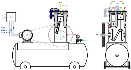
Figure 2.
Sensors’ locations in the RC. The accelerometers are denoted as A1, A2, A3, and A4.
4.2.1. Faults of the Reciprocal Compressor
The test bed enables the configuration of a set of 17 fault conditions concerning the valves. Four faults were configured for compressor stages and the discharge and inlet valves. The faults configured were (a) valve seat wear, (b) corrosion of the valve plate, (c) fracture of the valve plate, and broken spring. Table 2 presents the completed list of configured faults.
Table 2.
Valve faults in the RC.
4.2.2. RC Vibration Signal Dataset
Each vibration signal has a duration of 10 s. The motor rotated at 3462 rpm, representing a crankshaft rotation of 768 rpm. The operating conditions of the RC were kept constant during the vibration signal acquisition. In particular, the tank pressure was kept at 3 bar, the inlet pressure and discharge pressure were kept within the nominal range, and the surface temperature of the valve cover was maintained. Similarly, the environmental conditions corresponding to the room temperature and relative humidity were maintained within a predefined range. A total of 15 vibration signals were acquired for each fault condition, and a total of 255 vibration signals were acquired for each sensor.
5. Feature Extraction from the CP
5.1. Non-Linear Entropy Based Features
Each vibration signal in the CP dataset was processed for extracting a set of 29 features. The set of features was composed of a subset of 14 features corresponding to non-linear entropy features (Table A2) defined in Equations (A1)–(A14), a subset of 15 features corresponding to information-based features (Table A3) defined in Equations (A15)–(A29). The first step consisted of performing the phase space reconstruction [48] for estimating the spatial dimensions m and the lag of the system. The entropy-based features were estimated using these parameters. Each feature set estimated in a widow was considered a feature sample. Five non-contiguous segments of size 12,000 samples from each vibration signal were considered for calculating features. As the number of vibration signals files was 780, the total number of feature samples was .
5.2. Statistical Features
Additionally, a set of 12 statistical features (Table A4), defined in Equations (A30)–(A41), were extracted to compare to the entropy features set and be combined with other feature sets to evaluate their accuracy. The procedure for extracting the statistical features was similar to extracting the non-linear features. Three-thousand nine-hundred (3900) samples for the CP dataset were extracted and considered for classification.
6. Feature Extraction from the RC
6.1. Entropy Based Features
The procedure for extracting the features from the RC was similar to extracting the features from the CP. However, the number of segments with 12,000 samples was increased to ten. This increment was justified because this dataset had fewer files (255). A set of 29 entropy-based features was extracted from each signal segment. In total, 2550 feature samples were obtained for this dataset.
6.2. Statistical Features
A set of 2550 feature samples was obtained from the RC vibration signal dataset. The procedure was similar to the case of the CP. Each feature sample comprised 12 statistical features extracted from each of the windows considered, and each signal was subdivided into ten fragments.
7. Classification of Faults Using RF and SVM
Each feature dataset was used as input to both classical machine learning algorithms. Each dataset was randomly split into a training set (85%) and a test set (15%). The training set was used for 10-fold cross-validation, and the accuracy of the partitioned trained model was calculated with the test set. This entire process (including the splitting) was repeated ten times, and the accuracy is the average obtained during the repetitions.
The accuracy and the area under the Receiver Operator Curve (ROC) are two relevant metrics for classifier performance. Several metrics [79] were used for evaluating the classification results. The confusion matrix elements were used for defining the metrics [80].
8. Results
8.1. Results for the CP Dataset
The set of fault conditions for the CP included several severity levels in the impeller (see Table 1). Examples of the vibration signals for the CP dataset are shown in Figure 3. Four conditions are shown, and in this subset, only subtle differences in signal amplitude can be visually detected. Any fault signature could be affected by noise.
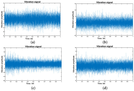
Figure 3.
Vibration signals from the CP dataset. (a) Signal from class P1. (b) Signal from class P6. (c) Signal from class P10, (d) Signal from class P13.
In Figure 4, the AppEn for four vibration signals of the CP dataset are shown. Each of the vibration signals represents a fault condition. The utility of non-linear features for detecting fault conditions in vibration signals is shown in the following paragraphs. The feature estimation in each signal starts by performing the phase space reconstruction [47] aimed at estimating the system dimension m and the lag . These parameters are used for calculating the AppEn for several values of r. The AppEn for the CP signals increases with r until attaining a maximum and decreases with the increase in r. In this example, the differences are evident between each impeller’s conditions.
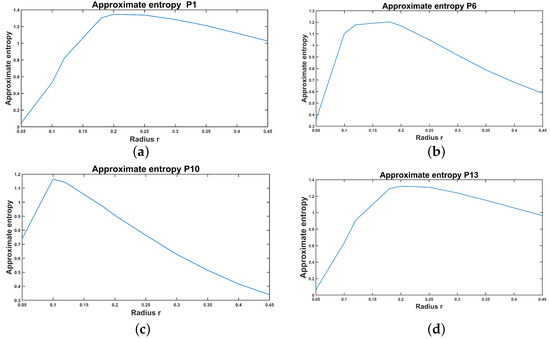
Figure 4.
AppEn for several signals from the pump dataset. (a) ApEn for a signal from class P1, (b) ApEn for a signal from class P6, (c) ApEn for a signal from class P10, (d) ApEn for a signal from class P13.
The LLE is calculated using four vibration signals extracted from the CP dataset. The calculation procedure was explained in Section 3.9. Results concerning the LLE are shown in Figure 5. The LLE is negative for the healthy class, class P6, and class P13. However, it is positive for class P10. The sign of the Lyapunov exponent could be related to the presence of chaos when the LLE is positive. When the LLE is negative, the time series could represent a system with periodic dynamics, as suggested in [65].
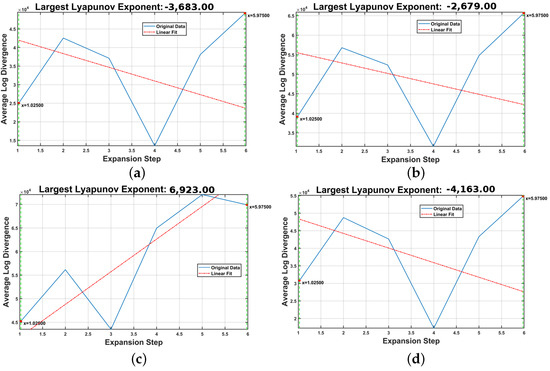
Figure 5.
LLE for several signals from the CP dataset. (a) LLE for class P1, (b) LLE for class P6, (c) LLE for class P10, (d) LLE for class P13.
A non-integer dimension usually characterizes non-linear systems that could have a chaotic nature. Generally, when dealing with chaotic systems, the Rényi dimension is used as a feature of strange attractors that enables the estimation of several feature dimensions. The is the fractal dimension, is the information dimension, and is the CD [81]. Like AppEn estimation, the first step corresponds to the phase space reconstruction that provides the embedding dimension m. Parameter m is the upper bound of the CD [82]. The CD feature was estimated for several vibration signals of the CP dataset. The results are shown in Figure 6. This set of signals has estimated embedding dimensions of 5 for P1 and P6, and 4 for P10 and P13. The CD is lower than 5 and higher than 4 for the signals from classes P1 and P6. Similarly, for classes P10, and P13, the CD values are higher than 3 and lower than 4.
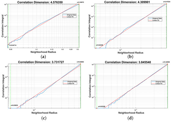
Figure 6.
CD for several signals from the CP dataset. (a) CD for a signal from class P1, (b) CD for a signal from class P6, (c) CD for a signal from class P10, (d) CD for a signal from class P13.
The percentages of accuracy for classifying the fault considering the CP dataset using RF and SVM are presented in Table 3. The accuracy is presented for each of the models and feature sets considered. The vibration signal channels A2, A3, and A4 were considered for feature extraction. Vibration signal channel A1 was not considered for two reasons. Firstly, the computational time of the feature extraction is high, and to keep the total feature extraction time feasible with the available hardware, we only considered three channels. Secondly, we selected the channels close to the mechanical connection with the motor, where a roller bearing is located, because the pump stages in this neighborhood have a higher probability of failing.
Table 3.
Percentages of accuracy for fault classification using the vibration signals of the CP dataset.
The lowest classification accuracy was attained using RF trained with the Statistical Features set. In this case, the accuracy attained from channel A2 was 67.76%, for channel A3 was 68.34%, and for channel A4 was 68.50%. The accuracy attained using SVM with this set of features was 68.5% for channel A2, 70.51% for channel A3, and 71.03% for channel A4. The highest accuracy was 99.59% for channel A2, 99.69% for channel A3, and 99.81% for channel A4. This accuracy was attained with the All Features set and SVM. With this set of features, using the RF model, the accuracy was 97.76% for channel A2, 99.38% for channel A3, and 99.37% for channel A4.
A comparison of accuracy considering both machine learning models and feature sets is presented in Figure 7. In the box plot, a red line represents the median of the data that divides the box or inter-quartile range in two parts. This box represents 50% of the data. The horizontal line over the box represents the upper quartile that indicates that 75% of the data have values below this quartile. The horizontal line below the box represents the lower quartile that indicates that 25% of the data have values below this quartile. The red cross below or over the box represents the outliers. The accuracy is presented for channel A2 in box plots calculated based on the ten repetitions performed for obtaining ten different cross-validated models. The highest accuracy (99.50% and 99.59% in Table 3) was attained based on the Entropy Features and the complete set of features, All Features, with the SVM model. The lower accuracies (67.76% and 68.50%) for the RF and SVM models were attained by considering the Statistical Features set. The combination of information entropy and statistical features (InfoStat Features) provided an intermediate accuracy value (84.60% and 86.96%) for both considered models.
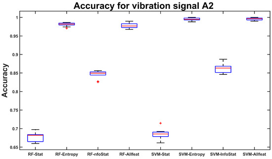
Figure 7.
Comparison of accuracy for the machine learning models tested, considering several combinations of features from channel A2 acquired from the CP.
Table 4 presents several performance metrics [79,80,83] results expressed in percentages. The included metrics are the sensitivity, the specificity, the error, the false positive rate, and the area under the curve (AUC). The metrics were calculated during the cross-validation results of the SVM model trained with the All Features set extracted from vibration signals recorded in the channel A2 from the CP. The highest sensitivity of 100.00% was attained by classes P1, P6, P12, and P13. In contrast, the lowest sensitivity of 98.67% was attained by class P9. The highest specificity of 100% was attained by classes P1, P3, P5, and P12. The lowest specificity of 99.87% was attained by classes P4 and P8. Concerning the AUC [84], the highest value of 100% was attained by classes P1 and P12, and the lowest AUC value was 99.19%.
Table 4.
Performance metrics (in percent) obtained with the SVM model and the All Features set. The model was trained using vibration signals in channel A2 from the CP dataset.
8.2. Results for the RC Dataset
A set of vibration signals for the RC is presented in Figure 8. The vibration signals presented are for the healthy class P1, and for class P6 representing the valve seat wear (in the inlet valve) of the second stage. The bottom row shows the vibration signal for class P11 corresponding to corrosion of the valve plate located in the discharge valve of the first stage. Finally, the vibration signal for the class P16 represents the fracture of the valve plate for inlet valve b of the first stage. The appearance of this vibration signal set differs from that of the CP dataset’s signals. In this dataset, the signals are more peaked, and each prominent peak indicating an event is surrounded by signals with lower amplitudes.
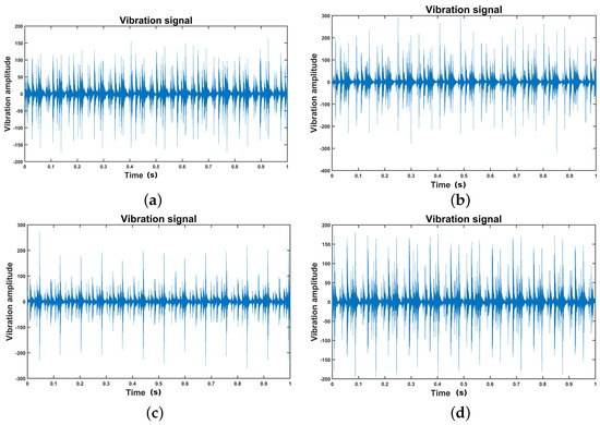
Figure 8.
Vibration signals from the RC dataset. (a) Signal from the class P1, (b) signal from class P6, (c) signal from class P11, (d) signal from class P16.
The AppEn estimated for each of the signals shown in Figure 8 is shown in Figure 9. The curve shape of AppEn is different from that of the CP. The AppEn in the RC is higher for low amplitudes and decreases as the threshold of amplitudes represented by the radius r increases.
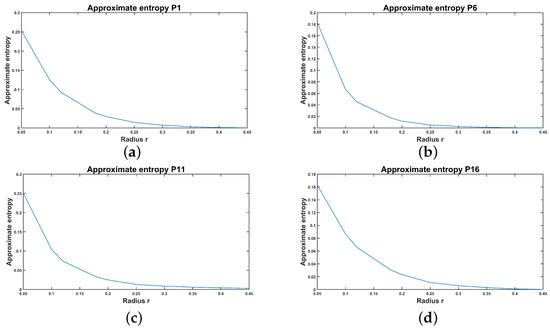
Figure 9.
AppEn for several signals from the RC dataset. (a) ApEn for a signal from the class P1, (b) ApEn for a signal from the class P6, (c) ApEn for a signal from the class P11, (d) ApEn for a signal from the class P16.
The calculation of the LLE for the set of vibration signals selected from the RC dataset is shown in Figure 10. Although the LLE value is different for each signal presented, all the estimated values are positive, suggesting that the system is chaotic [65]. The CD is presented in Figure 11 for the set of signals of the RC. The CD for these signals has different values according to the fault type. The estimated values of CD are close to the embedded dimensions [82] (four, calculated using the phase space reconstruction method).
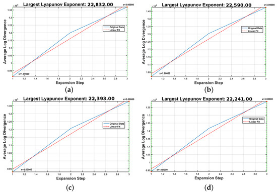
Figure 10.
LLE for several signals from the RC dataset. (a) LLE for class P1, (b) LLE for class P6, (c) LLE for a signal from the class P11, (d) LLE for class P16.
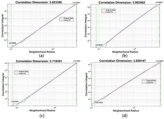
Figure 11.
CD for several signals from the RC dataset. (a) CD for a signal from the class P1, (b) CD for a signal from the class P6, (c) CD for a signal from the class P11, (d) CD for a signal from the class P16.
Concerning the RC, we selected three vibration channels from the four available. The selected channels were A1, A2, and A3. We excluded A4 to save computational time because A4 was far from the valve’s location. The percent accuracy attained using RF and SVM is presented in Table 5. Four feature sets are considered: the first is the Statistical Features set, and the second is the Entropy Features. The third is the InfoStat Features set. Finally, we have the All Features set. The lowest accuracy was attained with the Statistical Features set. In this case, the accuracy attained by the RF model was 83.96% for vibration signal channel A1, 74.07% for A2; and 72.33% for A3. The accuracy attained by the SVM model was 86.91% for vibration signal channel A1, 76.91% for A2, and 75.55% for A3. The highest accuracy was attained using the All Features set. The accuracy attained by the RF model was 95.35% for vibration signal channel A1, 94.40% for A2, and 88.82% for A3. The SVM model attained a classification accuracy of 97.90% for signal channel A1, 95.47% for A2 and 93.63% for A3. The rest of the feature combinations attained intermediate accuracy close to the optimal accuracy.
Table 5.
Percentage accuracy for fault classification using the vibration signals of the RC dataset.
A comparison of results obtained during the ten repetitions of the cross-validation is presented in Figure 12 for vibration signal A1. The comparison is presented using box plots. The accuracies attained by the Statistical Features set with RF and SVM were the lowest (83.96% and 86.91% in Table 5). The feature sets Entropy Features, InfoStat Features, and All Features attained higher accuracy with both machine learning models. In particular, the highest accuracies were attained by the All Features set with RF and SVM (95.35% and 97.90%). The accuracies attained by the Entropy Features were slightly lower, corresponding to 95.35% and 97.57% with the RD and SVM models, respectively. The accuracies attained by the InfoStat Features set were 93.96% and 96.83% with the RF and SVM models, respectively.
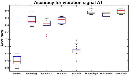
Figure 12.
Comparison of accuracy for the machine learning models tested, considering several combinations of features extracted from channel A1 of the RC dataset. In the box plot, a red line represents the median of the data. The horizontal line over the box represents the upper quartile. The horizontal line below the box represents the lower quartile. The red cross, below or over the box, represents the outliers.
A set of performance metrics [79,80,83] expressed in percentages is presented in Table 6. Such metrics were obtained with the SVM model trained with the All Features set extracted from vibration signals recorded in channel A1 from the RC dataset. The highest sensitivity of 100.00% was attained by classes P1, P2, P6, P7, P9, P10, and P11; and 93.99% attained by class P3 was the lowest. The highest specificity of 100% was attained by classes P1, P2, P10, and P17. The highest AUC value of 100.00% was attained by classes P1, P2, and P10; and the lowest value of 97.42% was attained by class P5.
Table 6.
Performance metrics (in percent) obtained with the SVM model and the All Features set. The model was trained using vibration signals in channel A1 from the RC dataset.
9. Discussion
The proposed methodology was implemented on a laptop computer. The laptop was equipped with an intel(R) Core(TM) i7-6700HQ CPU, 12 GB of RAM memory, and a graphics card NVIDIA GeForce GTX 950M. The Matlab software was used to implement the feature extraction and classification. Concerning the computational time, the Entropy Features set required an average time of 311.85 s when extracted from the five windows (each with a length of 12,000-time samples) of the vibration signals from the CP dataset. In contrast, the Information Entropy features require 0.97 s, and the Statistical Features set requires only 0.156 s. In the RC, when the sampling rate is similar to that of the CP and the window length is similar, the computational time is similar to the time required in the CP.
In the case of the CP, multiple pairwise comparisons of machine learning models are presented in Figure A1. A one-way analysis of variance by ranks was performed using a Kruskal–Wallis approach [85]. The test showed no significant statistical differences between results attained by either machine learning models when trained with the non-linear Entropy Features set or All Features set. Results attained by the SVM machine learning models trained with the non-linear Entropy Features set or the All Features set are statistically significantly superior to than those of RF or SVM models trained with the Statistical Features or the combination InfoStat Features. The comparison also shows that the non-linear Entropy Features set provides higher accuracy without combining with the Statistical Features set.
The plot representing the Kruskal–Wallis with multiple one-way comparisons is presented in Figure A2 for the RC. The combination of features corresponding to Entropy Features and All Features sets attained higher accuracies using both machine learning models, and there were no significant statistical differences between them. In contrast, there were significant statistical differences in the results attained with the Statistical Features set using both machine learning models. Additionally, the results obtained by the features sets Entropy Features, and All Features with the SVM model were statistically significantly superior to the results obtained with SVM using the InfoStat Features set.
A comparison with a deep-learning method was performed. For this purpose, the spectrogram of the vibration signal was calculated and fed to a CNN for fault classification. The spectrogram was calculated considering a Blackman widow of size 81.92 ms that was moved along the time axis with an overlap of 81.44 ms. The feature array had a size of , for each signal, and it was standardized using the Z-score normalization. The feature array for each dataset was fed to a CNN for 10-fold cross-validation. Results of the comparison are presented in Table 7. Concerning the case of the CP, the highest accuracy attained by the CNN was 98.86% for vibration channel A2, whereas using the Entropy Features set with SVM provided a classification accuracy of 99.50%. The accuracy attained by the RF model was 98.09%, which was slightly lower than the accuracy provided by the CNN. Results for the RC show that the highest accuracy attained by the CNN models was 96.74% when trained with signals from the A1 vibration channel. In contrast, the accuracy provided by the SVM trained with the Entropy Features extracted from the same channel was 97.57%. In summary, the accuracy provided by the SVM trained with the Entropy Features was higher than the accuracy attained by the CNN trained with the spectrogram of the vibration signal.
Table 7.
Comparison of performances of the tested models obtained during the 10-fold cross-validation between entropy features with classical models and the spectrogram with a CNN model.
Results can be compared to previous research that used non-linear entropy features with classical models. In [27], the average accuracy for classifying five different conditions in a CP was 94.58%. The work reported in [28] used an SVM for classifying four different conditions in a CP using vibration signals. The method attained an average accuracy of 98.4%. In [21] the , was used with LDA to classify six different conditions, attaining an accuracy of 99.62% in an RC. Several papers reported CNN-based approaches for fault classification in CP and RC [24,25,29,33]. These methods can highly accurately classify a small set of faults in a CP or an RC. In contrast, our method was able to classify 13 types of faults in a CP and 17 different conditions in an RC with accuracies close to those of these deep learning-based methods.
10. Conclusions
The non-linear Entropy Features set enables fault classification in a CP or an RC with high accuracy. In this research, 13 impeller faults in a CP incorporating different degrees of severity were classified using RF and SVM models. Additionally, a set of 17 valve faults in an RC were also classified.
The research showed that the non-linear Entropy Features set provides high accuracy (99.50% for the CP and 97.57% for the RC) considering the SVM model. The accuracy attained using the Entropy Features set and the RF model was 98.09% for the CP and 95.35% for the RC. Results showed no significant statistical differences between Entropy Features and All Features. However, both feature sets provided accuracies statistically significantly higher than the accuracy provided by the Statistical Features set. The Statistical Features set provided the lowest accuracy in this application. In this case, the accuracy attained with the SVM was 71.03% for the CP and 76.55% for the RC. Concerning the comparison of machine learning models, when both models RF and SVM were trained with the Entropy Features set, there were no statistically significant differences in the accuracy of results. The results suggest that the Entropy Features set or the All Features set could be used for fault classification in centrifugal pumps and reciprocating compressors, where multiple fault types in impellers and valves should be diagnosed at early stages.
The novelty of the approach is to propose using the entropy features for classifying faults in centrifugal pumps and reciprocating compressors with high accuracy. In addition, we showed that the entropy-based feature sets provide high classification accuracy even for a large number of faults in both the CP and the RC. Concerning the comparison with respect to a deep learning model, the accuracy results obtained by the SVM trained with the Entropy Features set (99.50% for the CP and 97.57% for the RC) were superior to those obtained by a CNN trained with the spectrogram (98.86% for the CP and 96.74% for the RC).
The limitation of the proposed approach is the high computational cost necessary for extracting the entire set of entropy-based features.
Further research is oriented at reducing the computational time required for extracting the non-linear Entropy Features set and exploring their implementation using multi-scale approaches. We also plan to select some of the entropy-based features that would be useful for anomaly detection in RM, combined with deep learning approaches, such as generative adversarial networks and autoencoders.
Author Contributions
Conceptualization, R.-V.S., M.C. and R.M.; methodology, D.C. and M.C.; software, R.M.; validation, R.M., E.E. and R.-V.S.; formal analysis, S.Y.; investigation, E.E.; resources, S.Y.; data curation, D.C.; writing—original draft preparation, R.M.; writing—review and editing, M.C. and R.-V.S.; visualization, D.C.; supervision, R.-V.S.; project administration, R.-V.S.; funding acquisition, R.-V.S. All authors have read and agreed to the published version of the manuscript.
Funding
This research was funded by the MoST Science and Technology Partnership Program (KY201802006) and National Research Base of Intelligent Manufacturing Service, Chongqing Technology and Business University, and by the Universidad Politécnica Salesiana through the GIDTEC research group.
Institutional Review Board Statement
Not applicable.
Informed Consent Statement
Not applicable.
Data Availability Statement
The data used in this research are available upon reasonable request to the corresponding authors. We also plan to prepare a paper describing the datasets and submit it to the MDPI journal Data to release them for public use.
Conflicts of Interest
The authors declare no conflict of interest.
Abbreviations
The following abbreviations are used in this manuscript:
| CP | Centrifugal Pump |
| RC | Reciprocating Compressor |
| CM | Condition Monitoring |
| CD | Correlation Dimension |
| LLE | Largest Lyapunov Exponent |
| LMD | Local Mean Decomposition |
| SVM | Support Vector Machine |
| CEEMD | Complementary Ensemble Empirical Mode Decomposition |
| SampEn | Sample Entropy |
| RF | Random Forest |
| ELM | Extreme Learning Machine |
| AMI | Average Mutual Information |
| FNN | False Nearest Neighbor |
| AppEn | Approximate Entropy |
| FuzzyEn | Fuzzy Entropy |
| ShannEn | Shannon Entropy |
| PermEn | Permutation Entropy |
| DFA | Detrended Fluctuation Analysis |
| LLE | Larger Lyapunov Exponent |
| Power Spectral Entropy | |
| PEB | Pitting at the Entrance of Impeller Blades |
| POB | Pitting at the Output of the Impeller Blades |
| ICB | Impeller Channel Blockage |
| IB | Imbalance Impeller |
| ROC | Receiver Operator Curve |
| AUC | Area Under the Curve |
| HP | Horse Power |
| RMS | Root Mean Square |
| RPM | Revolutions per minute |
| GPM | Gallons per minute |
| RM | Rotating Machinery |
| CNN | Convolutional Neural Network |
| SGWT | Spectral Graph Wavelet Transform |
| CECP | Complexity-Entropy Causality Plane |
| MSE | Multi-Scale Entropy |
| PCA | Principal Component Analysis |
| LDA | Linear Discriminant Analysis |
| BMFO | Binary Moth Flame Optimization |
| SE | Squeeze and Excitation |
| HYP | Hydraulic Pump |
| RSDD | Resonance-based sparse signal decomposition |
| MHAAPE | Multi-scale Hierarchical Amplitude Aware Permutation Entropy |
| ELM | Extreme Learning Machine |
| CEEMD | Complementary Ensemble Empirical Mode Decomposition |
| CWT | Continous Wavelet Transform |
| XBG | Extreme Gradient Boosting |
| AWT | Analitical Wavelet Transform |
Appendix A. Additional Tables
Appendix A.1. Related Research Compendium
Table A1.
Related research and characteristics.
Table A1.
Related research and characteristics.
| Contributors | Signal | Methods | Application | Advantages | Limitations |
|---|---|---|---|---|---|
| Li et al. [21] | Pressure | PCA | RC | Accuracy | Six types of fault |
| vibration | LDA | 99.62% | |||
| Patil et al. [23] | Vibration | BMFO | RC | Accuracy | Can get |
| Signal | KNN | > | trapped in | ||
| local minimum | |||||
| Lv et al. [22] | Pressure | ANN | RC | Accuracy | Several |
| 97.9% | Structuring | ||||
| Elements | |||||
| Zhao et al. [24] | Vibration | CNN | RC | Accuracy | Complex CNN |
| 99.4% | architecture | ||||
| Xiao et al. [25] | Vibration | CNN | RC | Acc = 100% | Complex CNN |
| Pressure | Architecture, | ||||
| Phase | 4 Conditions | ||||
| Ahmad et al. [28] | Vibration | SVM | CP | Accuracy | 4 conditions |
| 98.4% | |||||
| Hasan et al. [29] | Vibration | CNN | CP | Acc = 100% | 4 conditions |
| Ahmad et al. [30] | Vibration | KNN | CP | Acc = 100% | 4 conditions |
| Irfan et al. [31] | Voltage | XGB | Water pump | Acc = 100% | Threshold |
| Current | bearings | Selection | |||
| Kumar et al. [33] | Sound | CNN | CP | Sound Sensor | Acoustic noise |
| Zhao et al. [20] | Vibration | SVM | RC | Weak fault | LMD |
| MSE | detection | Mode mixing | |||
| Wang et al. [27] | Vibration | RF + CEEMD | CP | Accurate | High |
| SampEn | Comp. Cost | ||||
| Zhou et al. [26] | Vibration | RSDD + RF | HYP | Accurate | Large set |
| MHAAPE | of parameters | ||||
| Xin et al. [16] | Vibration | DFA + SGWT | RM | Retain fine | Lacks more |
| signatures | testing | ||||
| Radhakrishnan et al. [17] | Vibration | CECP + SVM | RM | Robust and | Setting of |
| easy | parameters |
Appendix A.2. Entropy-Based Features
Table A2.
Entropy features extracted.
Table A2.
Entropy features extracted.
| Feature | Equation | |
|---|---|---|
| ApEn [5,6] | (A1) | |
| ApEn [5,6] | (A2) | |
| FuzzyEn [10] | (A3) | |
| FuzzyEn [10] | (A4) | |
| SampEn [7] | (A5) | |
| SampEn [7] | (A6) | |
| ShannonEn [54] | (A7) | |
| CondEn [54] | (A8) | |
| CCondEn [54] | (A9) | |
| PermEn [57] | (A10) | |
| CorDim [59] | (A11) | |
| LLE [66] | (A12) | |
| DFA1( [66] | (A13) | |
| DFA2( [66] | (A14) |
Appendix A.3. Information-Based Features
Table A3.
Information entropy features.
Table A3.
Information entropy features.
| Feature | Equation | |
|---|---|---|
| WPT-Shannon [70,86] | (A15) | |
| WPT-Norm [70,86] | (A16) | |
| WPT-LogEn [70,86] | (A17) | |
| WPT-Thres [70,86] | (A18) | |
| WPT-Sure [70,86] | (A19) | |
| RényiEn [72] | (A20) | |
| TsallisEn [71] | (A21) | |
| PSE-mean [73,74] | (A22) | |
| PSE-std [73,74] | (A23) | |
| PSE-rms [73,74] | (A24) | |
| PSE-shape [73,74] | (A25) | |
| PSE-MaxToRms [73,74] | (A26) | |
| PSE-median [73,74] | (A27) | |
| PSE-Skew [73,74] | (A28) | |
| PSE-Kur [73,74] | (A29) |
Appendix A.4. Statistical Features
Table A4.
Statistical features.
Table A4.
Statistical features.
| Feature | Equation | |
|---|---|---|
| Mean | (A30) | |
| Root Mean Square (RMS) | (A31) | |
| Standard deviation | (A32) | |
| Kurtosis | (A33) | |
| Maximum value | (A34) | |
| Crest factor | (A35) | |
| Rectified mean value | (A36) | |
| Shape factor | (A37) | |
| Impulse factor | (A38) | |
| Variance | (A39) | |
| Minimum value | (A40) | |
| Skewness | (A41) |
Appendix B. Additional Figures
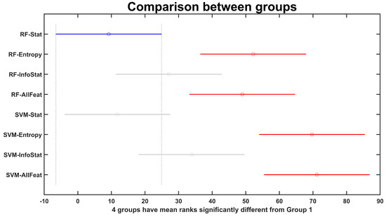
Figure A1.
Kruskal–Wallis comparison between the machine learning models tested. The plot shows several combinations of features calculated from the channel A2 recorded from the CP. There are statistical significant differences between the groups labeled with red and the group labeled with blue, between the groups SVM-Entropy and SVM-AllFeat and the groups labeled with blue and gray. In general there are statistically significant differences, when the projection of the horizontal lines of a group over the horizontal axis does not have any interception with the projection of another group.
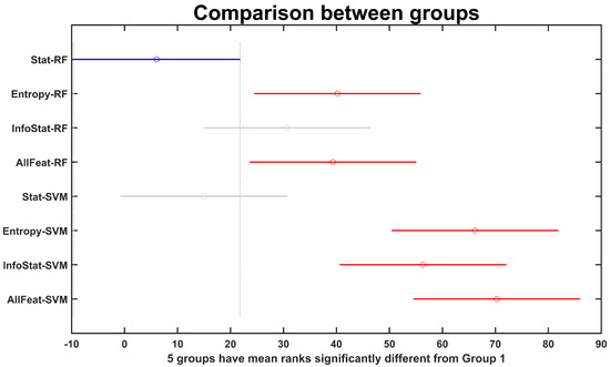
Figure A2.
Kruskal–Wallis comparison between the machine learning models tested, considering several combinations of features extracted from the channel A1 of the RC dataset. There are statistical significant differences between the groups labeled with red and the group labeled with blue. In general there are statistically significant differences, when the projection of the horizontal lines of a group over the horizontal axis does not have any interception with the projection of another group.
References
- Ali, S.M.; Hui, K.; Hee, L.; Leong, M.S. Automated valve fault detection based on acoustic emission parameters and support vector machine. Alex. Eng. J. 2018, 57, 491–498. [Google Scholar] [CrossRef]
- Cerrada, M.; Macancela, J.C.; Cabrera, D.; Estupiñan, E.; Sánchez, R.V.; Medina, R. Reciprocating compressor multi-fault classification using symbolic dynamics and complex correlation measure. Appl. Sci. 2020, 10, 2512. [Google Scholar] [CrossRef]
- Sharma, V.; Parey, A. Performance evaluation of decomposition methods to diagnose leakage in a reciprocating compressor under limited speed variation. Mech. Syst. Signal Process. 2019, 125, 275–287. [Google Scholar] [CrossRef]
- Soleimani, A.; Khadem, S. Early fault detection of rotating machinery through chaotic vibration feature extraction of experimental data sets. Chaos Solitons Fractals 2015, 78, 61–75. [Google Scholar] [CrossRef]
- Pincus, S.M. Approximate entropy as a measure of system complexity. Proc. Natl. Acad. Sci. USA 1991, 88, 2297–2301. [Google Scholar] [CrossRef]
- Pincus, S.M.; Huang, W.M. Approximate entropy: Statistical properties and applications. Commun. Stat. Theory Methods 1992, 21, 3061–3077. [Google Scholar] [CrossRef]
- Richman, J.S.; Moorman, J.R. Physiological time-series analysis using approximate entropy and sample entropy. Am. J. Physiol. Heart Circ. Physiol. 2000, 278, H2039–H2049. [Google Scholar] [CrossRef]
- Weippert, M.; Behrens, M.; Rieger, A.; Behrens, K. Sample entropy and traditional measures of heart rate dynamics reveal different modes of cardiovascular control during low intensity exercise. Entropy 2014, 16, 5698–5711. [Google Scholar] [CrossRef]
- Zhao, L.; Wei, S.; Zhang, C.; Zhang, Y.; Jiang, X.; Liu, F.; Liu, C. Determination of sample entropy and fuzzy measure entropy parameters for distinguishing congestive heart failure from normal sinus rhythm subjects. Entropy 2015, 17, 6270–6288. [Google Scholar] [CrossRef]
- Chen, W.; Wang, Z.; Xie, H.; Yu, W. Characterization of surface EMG signal based on fuzzy entropy. IEEE Trans. Neural Syst. Rehabil. Eng. 2007, 15, 266–272. [Google Scholar] [CrossRef]
- Wang, Z.; Xue, X. Multi-class support vector machine. In Support Vector Machines Applications; Springer: Berlin/Heidelberg, Germany, 2014; pp. 23–48. [Google Scholar] [CrossRef]
- Escalera, S.; Pujol, O.; Radeva, P. On the decoding process in ternary error-correcting output codes. IEEE Trans. Pattern Anal. Mach. Intell. 2010, 32, 120–134. [Google Scholar] [CrossRef] [PubMed]
- Janjarasjitt, S.; Ocak, H.; Loparo, K. Bearing condition diagnosis and prognosis using applied nonlinear dynamical analysis of machine vibration signal. J. Sound Vib. 2008, 317, 112–126. [Google Scholar] [CrossRef]
- Sun, Y. Fault Detection in Dynamic Systems Using the Largest Lyapunov Exponent. Ph.D. Thesis, Texas A & M University, College Station, TX, USA, 2012. [Google Scholar]
- Medina, R.; Macancela, J.C.; Lucero, P.; Cabrera, D.; Sánchez, R.V.; Cerrada, M. Gear and bearing fault classification under different load and speed by using Poincaré plot features and SVM. J. Intell. Manuf. 2020, 33, 1031–1055. [Google Scholar] [CrossRef]
- Dong, X.; Li, G.; Jia, Y.; Li, B.; He, K. Non-iterative denoising algorithm for mechanical vibration signal using spectral graph wavelet transform and detrended fluctuation analysis. Mech. Syst. Signal Process. 2021, 149, 107202. [Google Scholar] [CrossRef]
- Radhakrishnan, S.; Lee, Y.T.T.; Rachuri, S.; Kamarthi, S. Complexity and entropy representation for machine component diagnostics. PLoS ONE 2019, 14, e0217919. [Google Scholar] [CrossRef]
- Li, Y.; Wang, X.; Liu, Z.; Liang, X.; Si, S. The entropy algorithm and its variants in the fault diagnosis of rotating machinery: A review. IEEE Access 2018, 6, 66723–66741. [Google Scholar] [CrossRef]
- Huo, Z.; Martínez-García, M.; Zhang, Y.; Yan, R.; Shu, L. Entropy measures in machine fault diagnosis: Insights and applications. IEEE Trans. Instrum. Meas. 2020, 69, 2607–2620. [Google Scholar] [CrossRef]
- Zhao, H.-Y.; Wang, J.-D.; Xing, J.-J.; Gao, Y.-Q. A feature extraction method based on LMD and MSE and its application for fault diagnosis of reciprocating compressor. J. Vibroeng. 2015, 17, 3515–3526. [Google Scholar]
- Li, X.; Ren, P.; Zhang, Z.; Jia, X.; Peng, X. A p−V Diagram Based Fault Identification for Compressor Valve by Means of Linear Discrimination Analysis. Machines 2022, 10, 53. [Google Scholar] [CrossRef]
- Lv, Q.; Cai, L.; Yu, X.; Ma, H.; Li, Y.; Shu, Y. An Automatic Fault Diagnosis Method for the Reciprocating Compressor Based on HMT and ANN. Appl. Sci. 2022, 12, 5182. [Google Scholar] [CrossRef]
- Patil, A.; Soni, G.; Prakash, A. A BMFO-KNN based intelligent fault detection approach for reciprocating compressor. Int. J. Syst. Assur. Eng. Manag. 2021, 1–13. [Google Scholar] [CrossRef]
- Zhao, D.; Liu, S.; Zhang, H.; Sun, X.; Wang, L.; Wei, Y. Intelligent fault diagnosis of reciprocating compressor based on attention mechanism assisted convolutional neural network via vibration signal rearrangement. Arab. J. Sci. Eng. 2021, 46, 7827–7840. [Google Scholar] [CrossRef]
- Xiao, S.; Nie, A.; Zhang, Z.; Liu, S.; Song, M.; Zhang, H. Fault Diagnosis of a Reciprocating Compressor Air Valve Based on Deep Learning. Appl. Sci. 2020, 10, 6596. [Google Scholar] [CrossRef]
- Zhou, F.; Liu, W.; Yang, X.; Shen, J.; Gong, P. A new method of health condition detection for hydraulic pump using enhanced whale optimization-resonance-based sparse signal decomposition and modified hierarchical amplitude-aware permutation entropy. Trans. Inst. Meas. Control 2021, 43, 3360–3376. [Google Scholar] [CrossRef]
- Wang, Y.; Lu, C.; Liu, H.; Wang, Y. Fault diagnosis for centrifugal pumps based on complementary ensemble empirical mode decomposition, sample entropy and random forest. In Proceedings of the 2016 12th World Congress on Intelligent Control and Automation (WCICA), Guilin, China, 12–15 June 2016; IEEE: Piscataway, NJ, USA, 2016; pp. 1317–1320. [Google Scholar] [CrossRef]
- Ahmad, Z.; Rai, A.; Maliuk, A.S.; Kim, J.M. Discriminant feature extraction for centrifugal pump fault diagnosis. IEEE Access 2020, 8, 165512–165528. [Google Scholar] [CrossRef]
- Hasan, M.J.; Rai, A.; Ahmad, Z.; Kim, J.M. A fault diagnosis framework for centrifugal pumps by scalogram-based imaging and deep learning. IEEE Access 2021, 9, 58052–58066. [Google Scholar] [CrossRef]
- Ahmad, Z.; Nguyen, T.K.; Ahmad, S.; Nguyen, C.D.; Kim, J.M. Multistage centrifugal pump fault diagnosis using informative ratio principal component analysis. Sensors 2021, 22, 179. [Google Scholar] [CrossRef] [PubMed]
- Irfan, M.; Alwadie, A.S.; Glowacz, A.; Awais, M.; Rahman, S.; Khan, M.K.A.; Jalalah, M.; Alshorman, O.; Caesarendra, W. A novel feature extraction and fault detection technique for the intelligent fault identification of water pump bearings. Sensors 2021, 21, 4225. [Google Scholar] [CrossRef] [PubMed]
- Chen, T.; Guestrin, C. Xgboost: A scalable tree boosting system. In Proceedings of the 22nd ACM Sigkdd International Conference on Knowledge Discovery and Data Mining, San Francisco, CA, USA, 13–17 August 2016; pp. 785–794. [Google Scholar] [CrossRef]
- Kumar, A.; Gandhi, C.; Zhou, Y.; Kumar, R.; Xiang, J. Improved deep convolution neural network (CNN) for the identification of defects in the centrifugal pump using acoustic images. Appl. Acoust. 2020, 167, 107399. [Google Scholar] [CrossRef]
- Howedi, A.; Lotfi, A.; Pourabdollah, A. An entropy-based approach for anomaly detection in activities of daily living in the presence of a visitor. Entropy 2020, 22, 845. [Google Scholar] [CrossRef]
- Callegari, C.; Giordano, S.; Pagano, M. Entropy-based network anomaly detection. In Proceedings of the 2017 International Conference on Computing, Networking and Communications (ICNC), Santa Clara, CA, USA, 26–29 January 2017; IEEE: Piscataway, NJ, USA, 2017; pp. 334–340. [Google Scholar] [CrossRef]
- Palmieri, F. Network anomaly detection based on logistic regression of nonlinear chaotic invariants. J. Netw. Comput. Appl. 2019, 148, 102460. [Google Scholar] [CrossRef]
- Wu, S.; Moore, B.E.; Shah, M. Chaotic invariants of lagrangian particle trajectories for anomaly detection in crowded scenes. In Proceedings of the 2010 IEEE Computer Society Conference on Computer Vision and Pattern Recognition, San Francisco, CA, USA, 13–18 June 2010; IEEE: Piscataway, NJ, USA, 2010; pp. 2054–2060. [Google Scholar] [CrossRef]
- Garland, J.; Jones, T.R.; Neuder, M.; Morris, V.; White, J.W.; Bradley, E. Anomaly detection in paleoclimate records using permutation entropy. Entropy 2018, 20, 931. [Google Scholar] [CrossRef] [PubMed]
- Wang, S.; Lu, M.; Kong, S.; Ai, J. A Dynamic Anomaly Detection Approach Based on Permutation Entropy for Predicting Aging-Related Failures. Entropy 2020, 22, 1225. [Google Scholar] [CrossRef] [PubMed]
- Ahmad, S.; Styp-Rekowski, K.; Nedelkoski, S.; Kao, O. Autoencoder-based condition monitoring and anomaly detection method for rotating machines. In Proceedings of the 2020 IEEE International Conference on Big Data (Big Data), Atlanta, GA, USA, 10–13 December 2020; IEEE: Piscataway, NJ, USA, 2020; pp. 4093–4102. [Google Scholar] [CrossRef]
- de Paula Monteiro, R.; Lozada, M.C.; Mendieta, D.R.C.; Loja, R.V.S.; Bastos Filho, C.J.A. A hybrid prototype selection-based deep learning approach for anomaly detection in industrial machines. Expert Syst. Appl. 2022, 204, 117528. [Google Scholar] [CrossRef]
- Li, D.; Chen, D.; Jin, B.; Shi, L.; Goh, J.; Ng, S.K. MAD-GAN: Multivariate anomaly detection for time series data with generative adversarial networks. In Proceedings of the International Conference on Artificial Neural Networks, Munich, Germany, 17–19 September 2019; Springer: Berlin/Heidelberg, Germany, 2019; pp. 703–716. [Google Scholar] [CrossRef]
- Kumar, S.R.; Iniyal, U.; Harshitha, V.; Abinaya, M.; Janani, J.; Jayaprasanth, D. Anomaly Detection in Centrifugal Pumps Using Model Based Approach. In Proceedings of the 2022 8th International Conference on Advanced Computing and Communication Systems (ICACCS), Coimbatore, India, 25–26 March 2022; IEEE: Piscataway, NJ, USA, 2022; Volume 1, pp. 427–433. [Google Scholar] [CrossRef]
- Dutta, N.; Kaliannan, P.; Subramaniam, U. Application of machine learning algorithm for anomaly detection for industrial pumps. In Machine Learning Algorithms for Industrial Applications; Springer: Berlin/Heidelberg, Germany, 2021; pp. 237–263. [Google Scholar] [CrossRef]
- Dutta, A.; Karimi, I.A.; Farooq, S. PROAD (Process Advisor): A Health Monitoring Framework for Centrifugal Pumps. Comput. Chem. Eng. 2022, 163, 107825. [Google Scholar] [CrossRef]
- Charoenchitt, C.; Tangamchit, P. Anomaly Detection of a Reciprocating Compressor using Autoencoders. In Proceedings of the 2021 Second International Symposium on Instrumentation, Control, Artificial Intelligence, and Robotics (ICA-SYMP), Bangkok, Thailand, 20–22 January 2021; IEEE: Piscataway, NJ, USA, 2021; pp. 1–4. [Google Scholar] [CrossRef]
- Rand, D.; Young, L.S. Dynamical Systems and Turbulence. In Lecture Notes in Mathematics; Springer: Cham, Switzerland, 1981; Volume 898. [Google Scholar] [CrossRef]
- Vlachos, I.; Kugiumtzis, D. State space reconstruction for multivariate time series prediction. arXiv 2008, arXiv:0809.2220. [Google Scholar] [CrossRef]
- Abarbanel, H.D.; Brown, R.; Sidorowich, J.J.; Tsimring, L.S. The analysis of observed chaotic data in physical systems. Rev. Mod. Phys. 1993, 65, 1331. [Google Scholar] [CrossRef]
- Fraser, A.M.; Swinney, H.L. Independent coordinates for strange attractors from mutual information. Phys. Rev. A 1986, 33, 1134. [Google Scholar] [CrossRef]
- Kennel, M.B.; Brown, R.; Abarbanel, H.D. Determining embedding dimension for phase-space reconstruction using a geometrical construction. Phys. Rev. A 1992, 45, 3403. [Google Scholar] [CrossRef]
- Ribeiro, M.; Henriques, T.; Castro, L.; Souto, A.; Antunes, L.; Costa-Santos, C.; Teixeira, A. The entropy universe. Entropy 2021, 23, 222. [Google Scholar] [CrossRef] [PubMed]
- Azami, H.; Escudero, J. Amplitude-and fluctuation-based dispersion entropy. Entropy 2018, 20, 210. [Google Scholar] [CrossRef] [PubMed]
- Porta, A.; Baselli, G.; Liberati, D.; Montano, N.; Cogliati, C.; Gnecchi-Ruscone, T.; Malliani, A.; Cerutti, S. Measuring regularity by means of a corrected conditional entropy in sympathetic outflow. Biol. Cybern. 1998, 78, 71–78. [Google Scholar] [CrossRef]
- Feutrill, A.; Roughan, M. A Review of Shannon and Differential Entropy Rate Estimation. Entropy 2021, 23, 1046. [Google Scholar] [CrossRef] [PubMed]
- Bandt, C.; Pompe, B. Permutation entropy: A natural complexity measure for time series. Phys. Rev. Lett. 2002, 88, 174102. [Google Scholar] [CrossRef]
- Unakafova, V.A.; Keller, K. Efficiently measuring complexity on the basis of real-world data. Entropy 2013, 15, 4392–4415. [Google Scholar] [CrossRef]
- Steven, V. Heart rate variability linear and nonlinear analysis with applications in human physiology. Diss. Abstr. Int. 2010, 71. [Google Scholar]
- Lu, C.; Sun, Q.; Tao, L.; Liu, H.; Lu, C. Bearing health assessment based on chaotic characteristics. Shock Vib. 2013, 20, 519–530. [Google Scholar] [CrossRef]
- Rolo-Naranjo, A.; Montesino-Otero, M.E. A method for the correlation dimension estimation for on-line condition monitoring of large rotating machinery. Mech. Syst. Signal Process. 2005, 19, 939–954. [Google Scholar] [CrossRef]
- Ihlen, E.A. Introduction to multifractal detrended fluctuation analysis in Matlab. Front. Physiol. 2012, 3, 141. [Google Scholar] [CrossRef]
- JiaQing, W.; Han, X.; Yong, L.; Tao, W.; Zengbing, X. Detrended Fluctuation Analysis and Hough Transform Based Self-Adaptation Double-Scale Feature Extraction of Gear Vibration Signals. Shock Vib. 2016, 2016, 3409897. [Google Scholar] [CrossRef]
- Golińska, A.K. Detrended fluctuation analysis (DFA) in biomedical signal processing: Selected examples. Stud. Log. Gramm. Rhetor. 2012, 29, 107–115. [Google Scholar]
- Henry, B.; Lovell, N.; Camacho, F. Nonlinear dynamics time series analysis. In Nonlinear Biomedical Signal Processing: Dynamic Analysis and Modeling; Wiley: Hoboken, NJ, USA, 2012; Volume 2, pp. 1–39. [Google Scholar] [CrossRef]
- Wolf, A.; Swift, J.B.; Swinney, H.L.; Vastano, J.A. Determining Lyapunov exponents from a time series. Phys. D Nonlinear Phenom. 1985, 16, 285–317. [Google Scholar] [CrossRef]
- Rosenstein, M.T.; Collins, J.J.; De Luca, C.J. A practical method for calculating largest Lyapunov exponents from small data sets. Phys. D Nonlinear Phenom. 1993, 65, 117–134. [Google Scholar] [CrossRef]
- Shannon, C.E. A mathematical theory of communication. ACM SIGMOBILE Mob. Comput. Commun. Rev. 2001, 5, 3–55. [Google Scholar] [CrossRef]
- Gao, J.; Liu, F.; Zhang, J.; Hu, J.; Cao, Y. Information entropy as a basic building block of complexity theory. Entropy 2013, 15, 3396–3418. [Google Scholar] [CrossRef]
- Goldstein, S.; Lebowitz, J.L.; Tumulka, R.; Zanghì, N. Gibbs and Boltzmann entropy in classical and quantum mechanics. arXiv 2019, arXiv:1903.11870. [Google Scholar] [CrossRef]
- Coifman, R.R.; Wickerhauser, M.V. Entropy-based algorithms for best basis selection. IEEE Trans. Inf. Theory 1992, 38, 713–718. [Google Scholar] [CrossRef]
- Tsallis, C. Possible generalization of Boltzmann-Gibbs statistics. J. Stat. Phys. 1988, 52, 479–487. [Google Scholar] [CrossRef]
- Rényi, A. On measures of entropy and information. In Contributions to the Theory of Statistics, Proceedings of the Fourth Berkeley Symposium on Mathematical Statistics and Probability, Davis, CA, USA, 20–30 June 1960; The Regents of the University of California: Davis, CA, USA, 1961; Volume 1. [Google Scholar]
- Sharma, V.; Parey, A. A review of gear fault diagnosis using various condition indicators. Procedia Eng. 2016, 144, 253–263. [Google Scholar] [CrossRef]
- Pan, Y.; Chen, J.; Li, X. Spectral entropy: A complementary index for rolling element bearing performance degradation assessment. Proc. Inst. Mech. Eng. Part C J. Mech. Eng. Sci. 2009, 223, 1223–1231. [Google Scholar] [CrossRef]
- Breiman, L. Random forests. Mach. Learn. 2001, 45, 5–32. [Google Scholar] [CrossRef]
- Efron, B.; Tibshirani, R.J. An Introduction to the Bootstrap; CRC Press: Boca Raton, FL, USA, 1994. [Google Scholar]
- Vapnik, V.N. An overview of statistical learning theory. IEEE Trans. Neural Netw. 1999, 10, 988–999. [Google Scholar] [CrossRef] [PubMed]
- Scholkopf, B. Support vector machines: A practical consequence of learning theory. IEEE Intell. Syst. 1998, 13, 4. [Google Scholar] [CrossRef]
- Hossin, M.; Sulaiman, M. A review on evaluation metrics for data classification evaluations. Int. J. Data Min. Knowl. Manag. Process 2015, 5, 1. [Google Scholar] [CrossRef]
- Sokolova, M.; Lapalme, G. A systematic analysis of performance measures for classification tasks. Inf. Process. Manag. 2009, 45, 427–437. [Google Scholar] [CrossRef]
- Wang, W.; Chen, J.; Wu, Z. The application of a correlation dimension in large rotating machinery fault diagnosis. Proc. Inst. Mech. Eng. Part C J. Mech. Eng. Sci. 2000, 214, 921–930. [Google Scholar] [CrossRef]
- Boon, M.Y.; Henry, B.I.; Suttle, C.M.; Dain, S.J. The correlation dimension: A useful objective measure of the transient visual evoked potential? J. Vis. 2008, 8, 6. [Google Scholar] [CrossRef]
- Brown, J. Classifiers and their metrics quantified. Mol. Inform. 2018, 37, 1700127. [Google Scholar] [CrossRef]
- Bradley, A.P. The use of the area under the ROC curve in the evaluation of machine learning algorithms. Pattern Recognit. 1997, 30, 1145–1159. [Google Scholar] [CrossRef]
- Pohlert, T. The pairwise multiple comparison of mean ranks package (PMCMR). R Package 2014, 27, 9. [Google Scholar]
- Leite, G.d.N.P.; Araújo, A.M.; Rosas, P.A.C.; Stosic, T.; Stosic, B. Entropy measures for early detection of bearing faults. Phys. A Stat. Mech. Its Appl. 2019, 514, 458–472. [Google Scholar] [CrossRef]
Publisher’s Note: MDPI stays neutral with regard to jurisdictional claims in published maps and institutional affiliations. |
© 2022 by the authors. Licensee MDPI, Basel, Switzerland. This article is an open access article distributed under the terms and conditions of the Creative Commons Attribution (CC BY) license (https://creativecommons.org/licenses/by/4.0/).