Article

On Hermite Functions, Integral Kernels, and Quantum Wires

1
Centro Europeo Ricerche in Fisica Matematica (CERFIM), P.O. Box 1132, CH-6601 Locarno, Switzerland
2
Dipartimento di Scienze Ingegneristiche, Università degli Studi Guglielmo Marconi, Via Plinio 44, I-00193 Rome, Italy
3
Departamento de Física Teórica, Atómica y Óptica, and IMUVA, Universidad de Valladolid, 47011 Valladolid, Spain
*
Author to whom correspondence should be addressed.
Mathematics 2022, 10(16), 3012; https://doi.org/10.3390/math10163012
Submission received: 26 July 2022 / Revised: 10 August 2022 / Accepted: 18 August 2022 / Published: 21 August 2022
(This article belongs to the Special Issue Applications of Functional Analysis in Quantum Physics)

Abstract

:
In this note, we first evaluate and subsequently achieve a rather accurate approximation of a scalar product, the calculation of which is essential in order to determine the ground state energy in a two-dimensional quantum model. This scalar product involves an integral operator defined in terms of the eigenfunctions of the harmonic oscillator, expressed in terms of the well-known Hermite polynomials, so that some rather sophisticated mathematical tools are required.

1. Introduction

The present note will attempt to establish a connection between Hermite functions, integral operators, and solutions of two-dimensional quasi-solvable quantum models, with the discussion of some mathematical properties that arise in the study of a specific model. A first motivation for the present investigation comes after the following: in 1929, Plancherel and Rotach published a remarkable article on the asymptotic properties of Hermite polynomials [1]. Plancherel’s findings enabled B. Simon to investigate in depth the decay properties of the sequences of both the pointwise value and the supremum norm of the eigenfunctions of the harmonic oscillator [2] four decades later in [3]. Some generalisations of Hermite functions have been discussed in the literature [4]. Hermite functions are the eigenfunctions of the quantum harmonic oscillator and, therefore, they appear as an ingredient in the kernels of integral operators for models that use the harmonic oscillator. Apart from representing one of the fundamental topics in Functional Analysis and Operator Theory, integral operators have played a crucial role in several areas of Applied Mathematics for more than a century.
The analysis of solvable or quasi-solvable models in Quantum Mechanics is very useful in order to study properties of quantum objects as well as making approximations valid for a wide range of systems. Solvable models such as the one-dimensional square well or the harmonic oscillator serve as essential tools in the teaching of quantum mechanics. Point potentials are also typical solvable models, which serve as a laboratory to investigate bound states, scattering, resonances, self-adjoint determinations, etc. [5,6].
Quasi-solvable models are those that permit approximate solutions of the spectral problem for the Hamiltonian, at least for a finite number of eigenvalues. Generally speaking, quasi-solvable models are far from trivial and often require sophisticated mathematical methods for their resolution and this even may include the solution for the ground state.
While many solvable models are one-dimensional, interesting quasi-solvable models arise in the two-dimensional world. Two-dimensional models are interesting both from the physical as well as the mathematical point of view. From the physical point of view, it is well known that a 3D material with a two-dimensional confinement is a quantum wire. A typical example of a quantum wire is a carbon nanotube, which is of great interest in the physics of materials. In the study of a quantum wire, one usually considers the limiting case of a two-dimensional layer with a one-dimensional confining potential. Furthermore, two-dimensional systems are important in the physics of materials due to the properties of graphene or other kinds of thin films. From the mathematical point of view, two-dimensional models are often much more challenging than one-dimensional or three-dimensional ones. Some of these difficulties have their origin in the existence of a logarithmic singularity in the resolvent kernel of the free two-dimensional Laplacian [5,7]. In addition, point interactions in dimensions higher than one usually require renormalisation. Moreover, while point perturbations of the negative free Laplacian in both one and three dimensions may admit bound states for the attractive case only, two-dimensional point interactions may admit a bound state even if the interaction is repulsive [5,7]. In the case of point perturbations of the Hamiltonian of the harmonic oscillator, the striking difference characterising the two-dimensional model is given by the fact that the so-called level crossings of eigenvalues do not occur at the same value of the coupling constant, as fully shown in [8,9]. These are some of the facts that make the study of two-dimensional quantum models interesting and attractive.
In recent papers [10,11], we have considered a two-dimensional quasi-solvable model that combines several properties such as simplicity in the Hamiltonian with a mathematical complexity to solve the eigenvalue problem associated to this Hamiltonian, even for the calculation of the energy of the ground state, which is already a real challenge. In addition, this model serves as a two-dimensional limit for a quantum wire. This is a two-dimensional generalisation of the one-dimensional Hamiltonian H : = d 2 / d x 2 λ e x 2 , λ > 0 , which has received attention due to its quasi-solvability [12]. A slight generalisation of this one-dimensional Hamiltonian, say H : = d 2 / d x 2 + x 2 λ e x 2 , λ > 0 , is also quasi-solvable and the lowest energy eigenvalues have been obtained using the properties of the Birman–Schwinger operator [13]. Let us briefly describe this two-dimensional model and the technique used for its resolution. The point of departure is a free Hamiltonian given by
H 0 = 1 2 d 2 d x 2 + x 2 1 2 d 2 d y 2 .
It is to be noted that H 0 has no spatial symmetry with respect to the variables: while we have a harmonic oscillator in the x-variable, the motion with respect to the y-variable is that of a free particle. Then, we introduce an attractive isotropic Gaussian perturbation with coupling constant λ > 0 , so that the total Hamiltonian is
H λ : = H 0 λ e ( x 2 + y 2 ) .
As shown in [10], this Hamiltonian, H λ , is self-adjoint in the sense of quadratic forms, which implies that Q ( H λ ) Q ( H 0 ) Q ( A ) representing the quadratic form for the operator A, as fully explained in [14]), and is bounded from below. In order to estimate the spectrum of H λ , let us set V : = e ( x 2 + y 2 ) and consider the following Birman–Schwinger operator (see [15,16,17,18]):
B E : = V 1 / 2 ( H 0 E ) V 1 / 2 , E ρ ( H 0 ) ,
where ρ ( H 0 ) means the resolvent (complex numbers which are not in the spectrum, see [14]) of H 0 . In the present case, this operator is Hilbert–Schmidt (for a pedagogical introduction to trace ideals of bounded operators, we refer the reader to [14,15]). This fact shows that the eigenvalues of H λ are the zeros of the modified Fredholm determinant, which are the values of E for which
det 2 [ I λ B E ] = 0 ,
where for any Hilbert–Schmidt operator A, we define the modified Fredholm determinant as det 2 [ I + A ] : = det [ I + A ] e Tr A , where det [ I + A ] is the ordinary Fredholm determinant [5,19,20] and I the identity operator. Note that A either could be or could not be trace class.
The Birman–Schwinger operator (3) is an integral operator with integral kernel given by
B E ( x , x , y , y ) = e ( x 2 + y 2 ) / 2 n = 0 e γ n ( E ) | y y | γ n ( E ) ϕ n ( x ) ϕ n ( x ) e ( x 2 + y 2 ) / 2 = n = 0 K E , n ( x , x , y , y ) ,
where the meaning of each of the K E , n ( x , x , y , y ) is obvious and the functions ϕ n ( x ) are the L 2 ( R ) normalised Hermite functions
ϕ n ( x ) = 1 2 n n ! π e x 2 / 2 H n ( x ) ,
H n ( x ) being the well-known Hermite polynomials [2]. Here, we see the relation between Hermite functions and integral kernels mentioned earlier and that is specific for the present model. The functions γ n ( E ) are given by
γ n ( E ) = 2 n + 1 2 E , n = 0 , 1 , 2 ,
As was done in [11], for a given value of the coupling constant λ , the energy of the ground state is given by E 0 ( λ ) = 1 2 ϵ 0 ( λ ) , with ϵ 0 > 0 . Then, γ 0 ( ϵ 0 ) = 2 ϵ 0 . For this value of E, the integral kernel, denoted by B ϵ 0 , can be divided for the sake of convenience into the sum of three terms [11]:
B ϵ 0 = P ϵ 0 + M ϵ 0 + N ϵ 0 ,
where P ϵ 0 (respectively M ϵ 0 ) is the integral kernel of a rank one (respective trace class) operator. The last term, N ϵ 0 , is the integral kernel of a positive Hilbert–Schmidt operator and has the following form (compare to (5)):
N ϵ 0 ( x , x , y , y ) = e ( x 2 + y 2 ) / 2 n = 1 e γ n ( ϵ 0 ) | y y | γ n ( ϵ 0 ) ϕ n ( x ) ϕ n ( x ) e ( x 2 + y 2 ) / 2 ,
with γ ( ϵ 0 ) = 2 ( n + ϵ 0 ) , n 1 .
The main objective of the present note is the study of some mathematical properties of the operator with integral kernel given by N ϵ 0 ( x , x , y , y ) .
From a broader mathematical point of view, due to the structure of the Kernels (5) and (9), it might be worth pointing out that our work can be regarded as a two-dimensional approximation method for convolutions using orthogonal functions, namely those of the harmonic oscillator. Other examples of two-dimensional approximation methods were dealt with in [21,22].

2. On the Mathematics of the Integral Kernel N ϵ 0 ( x , x , y , y )

From (5) and (9), we have that
N ϵ 0 ( x , x , y , y ) = n = 1 K ϵ 0 , n ( x , x , y , y ) ,
where the term with n = 0 in (5) contributes to the sum P ϵ 0 + M ϵ 0 .
We have already shown in [11] that, although each summand K ϵ 0 , n ( x , x , y , y ) is the integral kernel of a trace class operator, its sum N ϵ 0 ( x , x , y , y ) is not. Instead, N ϵ 0 ( x , x , y , y ) is the integral kernel of a Hilbert–Schmidt operator. In fact, as ϵ 0 0 + , the integral operator with kernel N ϵ 0 ( x , x , y , y ) converges in the Hilbert–Schmidt norm to another integral operator with kernel
N 0 ( x , x , y , y ) = e ( x 2 + y 2 ) / 2 n = 1 e 2 n | y y | 2 n e ( x 2 + y 2 ) / 2 ,
satisfying the following estimate:
Tr ( N ϵ 0 2 ) Tr ( N 0 2 ) π 3 2 4 n = 1 ϕ 2 n 2 ( 0 ) n 3 4 2 1.66265 ,
see [11].
By setting
f ϵ 0 ( n ) ( x , y ) = e x 2 / 2 ϕ n ( x ) e y 2 / 2 e 2 ( n + ϵ 0 ) | y | , n = 0 , 1 , 2 , ,
so that f 0 ( n ) : = lim ϵ 0 0 + f ϵ 0 ( n ) . We recall that the evaluation of the scalar product f 0 ( 0 ) , N 0 f 0 ( 0 ) was achieved in [11] by using the explicit Expression (11). Here, we wish to generalise that argument by estimating the following scalar product instead:
f ϵ 0 ( 0 ) , N 0 f ϵ 0 ( 0 ) = n = 1 R 4 f ϵ 0 ( 0 ) ( x , y ) K 0 , n ( x , x , y , y ) f ϵ 0 ( 0 ) ( x , y ) d x d x d y d y = n = 1 1 2 n R e x 2 ϕ 0 ( x ) ϕ n ( x ) d x 2 R 2 e y 2 2 ϵ 0 | y | e 2 n | y y | e y 2 2 ϵ 0 | y | d y d y = π n = 1 1 2 n R ϕ 0 3 ( x ) ϕ n ( x ) d x 2 R 2 e y 2 2 ϵ 0 | y | e 2 n | y y | e y 2 2 ϵ 0 | y | d y d y = π n = 1 1 2 n ϕ 0 , ϕ 0 2 ϕ n 2 R 2 e y 2 2 ϵ 0 | y | e 2 n | y y | e y 2 2 ϵ 0 | y | d y d y .
In [13], the following relations were established:
( ϕ 0 , ϕ 0 2 ϕ 2 n 1 ) = 0 , ( ϕ 0 , ϕ 0 2 ϕ 2 n ) = ϕ 2 n 2 ( 0 ) 2 2 n + 1 π , n = 1 , 2 ,
Thus,
f ϵ 0 ( 0 ) , N 0 f ϵ 0 ( 0 ) = π 4 n = 1 ϕ 2 n 2 ( 0 ) 2 2 n n R 2 e y 2 2 ϵ 0 | y | e 2 n | y y | e y 2 2 ϵ 0 | y | d y d y = π 4 n = 1 ϕ 2 n 2 ( 0 ) 2 2 n n R e y 2 2 ϵ 0 | y | e 2 n | · | * e ( · ) 2 2 ϵ 0 | · | ( y ) d y ,
where f * g denotes, as usual, the convolution between the functions f and g.
Next, let us find an upper and a lower bound for f ϵ 0 ( 0 ) , N 0 f ϵ 0 ( 0 ) using the right-hand side of (16). As a straightforward consequence of Young’s inequality regarding the convolution of two functions [15], we have:
e ( · ) 2 2 ϵ 0 | · | e 2 n | · | * e ( · ) 2 2 ϵ 0 | · | 2 e ( · ) 2 2 ϵ 0 | · | 2 e 2 n | · | * e ( · ) 2 2 ϵ 0 | · | 2 e ( · ) 2 2 ϵ 0 | · | 2 2 e 2 n | · | 1 = 2 n 0 e 2 ( y 2 + 2 ϵ 0 y ) d y = 2 e ϵ 0 n 0 e 2 ( y + ϵ 0 / 2 ) 2 d y = 2 e ϵ 0 n ϵ 0 2 e 2 y 2 d y = 2 n e ϵ 0 ϵ 0 e y 2 d y = π 2 n e ϵ 0 erfc ( ϵ 0 ) .
Thus, (16) is bounded from above by
π 2 2 e ϵ 0 erfc ( ϵ 0 ) n = 1 ϕ 2 n 2 ( 0 ) 2 2 n ( 2 n ) = π 8 ln ( 4 ( 2 3 ) ) e ϵ 0 erfc ϵ 0 .
The series in (18) converges rapidly due to the decay of ϕ 2 n 2 ( 0 ) 1 2 n , which is a consequence of the properties of Hermite polynomials, first established by Plancherel and Rotach [1] (see also [23,24,25,26,27]). Therefore, the general term in the series in (18) decays like 1 2 2 n ( 2 n ) 3 / 2 .
In order to obtain a lower bound for the scalar product f ϵ 0 ( 0 ) , N 0 f ϵ 0 ( 0 ) , we take into account that
e 2 n ( | y | + | y | ) e 2 n | y y | ,
and use Inequality (19) into the first series in (16), thus leading to the lower bound:
π 4 n = 1 ϕ 2 n 2 ( 0 ) 2 2 n n R e y 2 2 ( n + ϵ 0 / 2 ) | y | d y 2 = π n = 1 ϕ 2 n 2 ( 0 ) 2 2 n n 0 e y 2 2 ( n + ϵ 0 / 2 ) y d y 2 = π n = 1 ϕ 2 n 2 ( 0 ) 2 2 n n e ( n + ϵ 0 / 2 ) 2 0 e y + n + ϵ 0 / 2 2 d y 2 = π n = 1 ϕ 2 n 2 ( 0 ) 2 2 n n e ( n + ϵ 0 / 2 ) 2 n + ϵ 0 / 2 e y 2 d y 2 .
Then, taking into account that 0 ϵ 0 1 , we obtain the following lower bound:
π 3 4 n = 1 ϕ 2 n 2 ( 0 ) 2 2 n n e 2 n erfc 2 n + 1 2 0.00006617 .
Next, we wish to obtain an analytical expression for f ϵ 0 ( 0 ) , N 0 f ϵ 0 ( 0 ) using the first series in (16), where a double integral appears. Let us solve this integral by splitting its calculation into two steps. First, we consider the integration over the first and third quadrant of the (x, y) plane:
I 1 , 3 = 0 0 e y 2 2 ϵ 0 y e 2 n | y y | e y 2 2 ϵ 0 y d y d y + 0 0 e y 2 + 2 ϵ 0 y e 2 n | y y | e y 2 + 2 ϵ 0 y d y d y = 0 0 e y 2 2 ϵ 0 y e 2 n | y y | e y 2 2 ϵ 0 y d y d y + 0 0 e y 2 + 2 ϵ 0 y e 2 n | y y | e y 2 + 2 ϵ 0 y d y d y = 2 0 0 e y 2 2 ϵ 0 y e 2 n | y y | e y 2 2 ϵ 0 y d y d y .
The y-integral can be split into two by writing explicitly the absolute value inside the exponent of the second exponential inside the integrand
I 1 , 3 = 2 0 e y 2 2 ϵ 0 y 0 y e 2 n ( y y ) e y 2 2 ϵ 0 y d y d y + 2 0 e y 2 2 ϵ 0 y y e 2 n ( y y ) e y 2 2 ϵ 0 y d y d y = 2 0 e y 2 2 ( n + ϵ 0 / 2 ) y 0 y e y 2 + 2 ( n ϵ 0 / 2 ) y d y d y + 2 0 e y 2 + 2 ( n ϵ 0 / 2 ) y y e y 2 2 ( n + ϵ 0 / 2 ) y d y d y = 2 e 2 n + ϵ 0 0 e ( y + n + ϵ 0 / 2 ) 2 0 y e ( y n + ϵ 0 / 2 ) 2 d y d y + 2 e 2 n + ϵ 0 0 e ( y n + ϵ 0 / 2 ) 2 y e ( y + n + ϵ 0 / 2 ) 2 d y d y .
The last term in (23) can be easily written in terms of the error function [2] as
π e 2 n + ϵ 0 0 e ( y n + ϵ 0 / 2 ) 2 erfc y + n + ϵ 0 / 2 d y ,
while the previous term can be treated by using integration by parts as follows:
2 e 2 n + ϵ 0 0 e ( y + n + ϵ 0 / 2 ) 2 0 y e ( y n + ϵ 0 / 2 ) 2 d y d y = π e 2 n + ϵ 0 0 d d y erfc y + n + ϵ 0 / 2 0 y e ( y n + ϵ 0 / 2 ) 2 d y d y = π e 2 n + ϵ 0 erfc y + n + ϵ 0 / 2 0 y e ( y n + ϵ 0 / 2 ) 2 d y 0 + π e 2 n + ϵ 0 0 erfc y + n + ϵ 0 / 2 d d y 0 y e ( y n + ϵ 0 / 2 ) 2 d y d y = π e 2 n + ϵ 0 0 e ( y n + ϵ 0 / 2 ) 2 erfc y + n + ϵ 0 / 2 d y .
By performing a simple change of variables, we see that the sum of (24) plus (25) gives:
I 1 , 3 = 2 π e 2 n + ϵ 0 ϵ 0 / 2 e ( y n ) 2 erfc y + n d y .
The contribution from the fourth quadrant to the double integral in (16) is
I 4 = 0 0 e y 2 2 ϵ 0 y e 2 n y + | y | e y 2 2 ϵ 0 y d y d y = 0 e y 2 2 n + ϵ 0 / 2 y d y 0 e y 2 2 n + ϵ 0 / 2 | y | d y = 0 e y 2 2 n + ϵ 0 / 2 y d y 2 = π 4 e 2 n + ϵ 0 / 2 2 erfc 2 n + ϵ 0 / 2 .
By means of simple symmetry arguments, it is immediate to infer that the contribution from the second quadrant I 2 is identical to I 4 , so that the double integral inside the sum on the right-hand side of (16) is equal to:
2 π e 2 n + ϵ 0 ϵ 0 / 2 e ( y n ) 2 erfc y + n d y + π 2 e 2 n + ϵ 0 / 2 2 erfc 2 n + ϵ 0 / 2 .
Hence, from the first series in (16), we obtain the following result:
f ϵ 0 ( 0 ) , N 0 f ϵ 0 ( 0 ) = π 2 n = 1 ϕ 2 n 2 ( 0 ) 2 2 n n e 2 n + ϵ 0 ϵ 0 / 2 e ( y n ) 2 erfc y + n d y + π 2 3 n = 1 ϕ 2 n 2 ( 0 ) 2 2 n n e 2 n + ϵ 0 / 2 2 erfc 2 ( n + ϵ 0 / 2 ) .
Let us consider the first summand in the above Expression (29). In order to make the function of ϵ 0 defined as the sum up to infinity more tractable, it might be convenient to replace it by its truncation up to n = 10, that is to say:
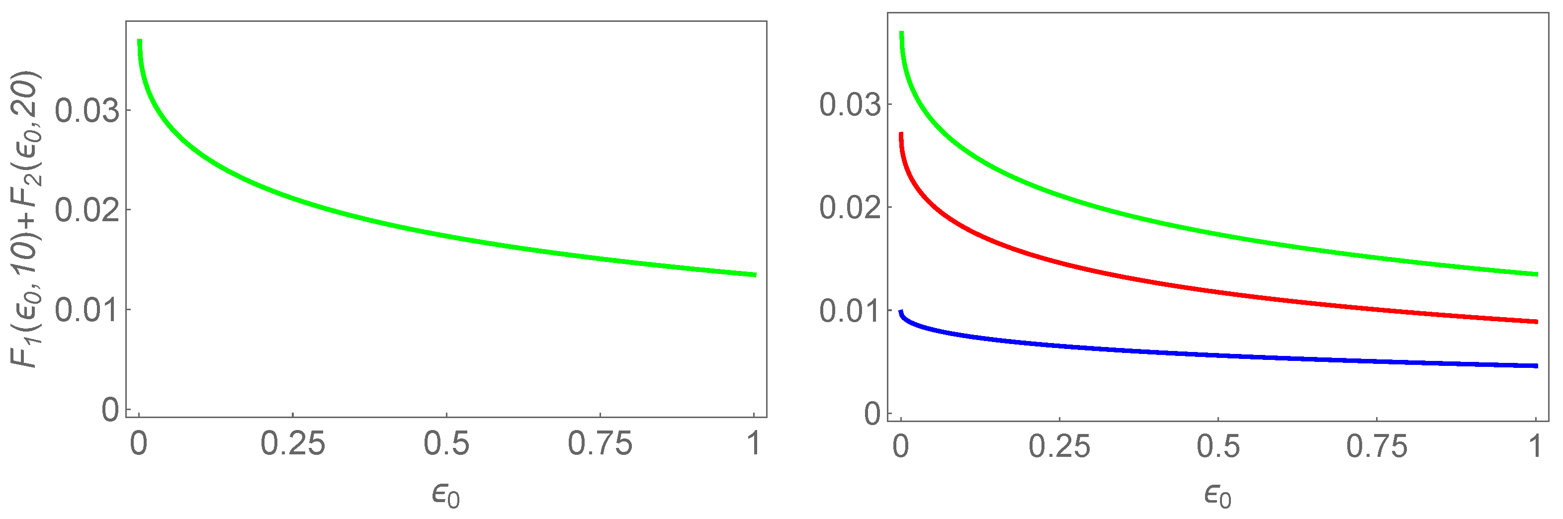
F 1 ( ϵ 0 , 10 ) : = π 2 n = 1 10 ϕ 2 n 2 ( 0 ) 2 2 n n e 2 n + ϵ 0 ϵ 0 / 2 e ( y n ) 2 erfc y + n d y .
In Figure 1, we provide the plot of F 1 ( ϵ 0 , 10 ) as a function of ϵ 0 for any ϵ 0 ( 0 , 1 ) .
Needless to say, we have to estimate the remainder, namely:
R 1 ( ϵ 0 , 11 ) : = π 2 n = 11 ϕ 2 n 2 ( 0 ) 2 2 n n e 2 n + ϵ 0 ϵ 0 / 2 e ( y n ) 2 erfc y + n d y .
Note that the right-hand side of (31) is always positive with ϵ 0 ( 0 , 1 ) , so that we have the following inequality:
R 1 ( ϵ 0 , 11 ) π e 2 n = 11 ϕ 2 n 2 ( 0 ) 2 2 n n e 2 n 0 e ( y n ) 2 erfc y + n d y = π e 2 n = 11 ϕ 2 n 2 ( 0 ) 2 2 n n e n 0 e y 2 + 2 n y erfc y + n d y = π e 2 n = 11 ϕ 2 n 2 ( 0 ) n e 4 n 0 e y 2 e 2 n y erfc y + n d y .
Observe that for any y 0 , we have that
d d y e 2 n y erfc y + n = 2 e 2 n y π π n erfc y + n e ( y + n ) 2 < 0 .
From here, it follows that the second factor inside each integrand is a decreasing function for any y 0 . Then, the last series in (32) is bounded from above by
π e 2 n = 11 ϕ 2 n 2 ( 0 ) n e 4 n erfc n 0 e y 2 d y = π 3 / 2 e 4 n = 11 ϕ 2 n 2 ( 0 ) n e 4 n erfc n 8.05813 × 10 10 ,
so that
R 1 ( ϵ 0 , 11 ) 8.05813 × 10 10 .
The convergence of the Series (34) is faster than the convergence of the geometric series. This is a consequence of the fact that ϕ 2 n 2 ( 0 ) / n decays like 1 n (see [23,24,25,26,27,28,29]), and that erfc n decays like e n / π n , as shown in [2].
Once we have estimated the first series in (29), we turn our attention to the evaluation of the second series. We split this series by truncating it up to n = 20 . This obviously gives
F 2 ( ϵ 0 , 20 ) : = π 2 3 n = 1 20 ϕ 2 n 2 ( 0 ) 2 2 n n e 2 n + ϵ 0 / 2 2 erfc 2 n + ϵ 0 / 2 .
In Figure 2, we plot F 2 ( ϵ 0 , 20 ) as a function of ϵ 0 ( 0 , 1 ) .
The remainder of this series, denoted by R 2 ( ϵ 0 , 21 ) , can be estimated as follows:
R 2 ( ϵ 0 , 21 ) π 2 3 n = 21 ϕ 2 n 2 ( 0 ) 2 2 n n e 2 n + 1 / 2 2 erfc 2 ( n ) = π 2 3 e n = 21 ϕ 2 n 2 ( 0 ) 2 2 n n e 2 n + 4 n / 2 erfc 2 ( n ) 5.78891 × 10 11 ,
as a consequence of the above considerations on the decay of ϕ 2 n 2 ( 0 ) / n and erfc n for large values of n, one concludes that
e 2 n + 4 n / 2 erfc 2 ( n ) 2 2 n < 1 π n e 4 n
for any n > 21 . Thus, the desired approximation is
f ϵ 0 ( 0 ) , N 0 f ϵ 0 ( 0 ) F 1 ( ϵ 0 , 10 ) + F 2 ( ϵ 0 , 20 ) .
We plot this approximation in terms of ϵ 0 in Figure 3.
Note that, by using (35) and (37), the estimation of the total error with the truncations used above is
R 1 ( ϵ 0 , 11 ) + R 2 ( ϵ 0 , 21 ) < 8.637021 × 10 10 .
Finally,
f 0 ( 0 ) , N 0 f 0 ( 0 ) = lim ϵ 0 0 f ϵ 0 ( 0 ) , N 0 f ϵ 0 ( 0 ) .
We conclude our discussion with this result.

3. Concluding Remarks

Quantum quasi-solvable models are important since they serve as approximations of realistic situations. In addition, two-dimensional quantum models describe properties of new materials such as graphene or any kind of thin films. Two-dimensional models are far more challenging from the mathematical point of view than their one or three-dimensional analogues. As is well known, the main reason for these difficulties is the logarithmic singularity at the origin of the integral kernel of the resolvent operator of the free Hamiltonian, known as Green’s function in the mathematical physics literature. This singular behaviour obviously affects the associated Birman–Schwinger operator, that is to say the integral operator enabling us to investigate the eigenvalues as well as the resonances of the Hamiltonian with the interaction under consideration.
As attested by our recent analysis of a two-dimensional model with the free Hamiltonian endowed with the harmonic confinement in one direction and the interaction represented by an isotropic Gaussian potential, the detailed study of the integral kernel of the related Birman–Schwinger operator relies crucially on the decay properties of the eigenfunctions of the harmonic oscillator. In some recent papers of ours, it was shown that such an operator is Hilbert–Schmidt, so that the functional-analytic tool known as modified Fredholm determinant is required in order to evaluate the two lowest energy eigenvalues of such a model.
One term of the modified Fredholm determinant is given by the scalar product investigated in detail in this note. Despite its challenging complexity, we have achieved to determine a rather manageable expression for it in terms of two series involving the complementary error function. Furthermore, after establishing the fast convergence of both series, we have obtained a highly accurate approximation by means of a suitable truncation of both series.

Author Contributions

Conceptualization, S.F., M.G. and F.R.; methodology, S.F., M.G., L.M.N. and F.R.; formal analysis, S.F., M.G. and F.R.; writing S.F., M.G. and F.R.; supervision, L.M.N.; project administration, L.M.N.; funding acquisition, L.M.N. All authors have read and agreed to the published version of the manuscript.

Funding

This research was funded by the Spanish Ministerio de Ciencia e Innovación (MCIN) with funding from the European Union NextGenerationEU (PRTR C17.I1) and the Consejería de Educación, Junta de Castilla y León, through QCAYLE project, as well as the PID2020-113406GB-I0 grant by MCIN.

Institutional Review Board Statement

Not applicable.

Informed Consent Statement

Not applicable.

Data Availability Statement

Not applicable.

Conflicts of Interest

The authors declare no conflict of interest.

References

  1. Plancherel, M.; Rotach, W. Sur les valeurs asymptotiques des polynomes d’Hermite H n ( x ) = ( I ) n e x 2 2 d n d x n ( e x 2 2 ) . Comment. Math. Helv. 1929, 227, 1. [Google Scholar]
  2. Arfken, G.B. Mathematical Methods for Physicists, 3rd ed.; Academic Press: Cambridge, MA, USA, 1985. [Google Scholar]
  3. Simon, B. Distributions and their Hermite expansion. J. Math. Phys. 1971, 12, 140. [Google Scholar] [CrossRef]
  4. Celeghini, E.; Gadella, M.; del Olmo, M.A. Symmetry Groups, Quantum Mechanics and Generalized Hermite Functions. Mathematics 2022, 10, 1448. [Google Scholar] [CrossRef]
  5. Albeverio, S.; Gesztesy, F.; Høeg-Krohn, R.; Holden, H. Solvable Models in Quantum Mechanics, 2nd ed.; AMS Chelsea Series; AMS: Providence, RI, USA, 2004. [Google Scholar]
  6. Albeverio, S.; Kurasov, P. Singular Perturbations of Differential Operators; Cambridge University Press: Cambridge, UK, 1999. [Google Scholar]
  7. Fassari, S.; Popov, I.; Rinaldi, F. On the behaviour of the two dimensional Hamiltonian −Δ + λ[δ(x + x0) + δ(xx0)] as the distance between the two centers vanishes. Phys. Scr. 2020, 95, 075209. [Google Scholar] [CrossRef]
  8. Fassari, S.; Gadella, M.; Glasser, M.L.; Nieto, L.M.; Rinaldi, F. Level crossings of eigenvalues of the Schrodinger Hamiltonian of the isotropic harmonic oscillator perturbed by a central point interaction in different dimensions. Nanosyst. Phys. Chem. Math. 2018, 9, 179–186. [Google Scholar] [CrossRef]
  9. Fassari, S.; Gadella, M.; Nieto, L.M.; Rinaldi, F. Spectral properties of the 2D Schrödinger Hamiltonian with various solvable confinements in the presence of a central point perturbation. Phys. Scr. 2019, 94, 055202. [Google Scholar] [CrossRef] [Green Version]
  10. Albeverio, S.; Fassari, S.; Gadella, M.; Nieto, L.M.; Rinaldi, F. The Birman-Schwinger operator for a parabolic quantum well in a zero-thickness layer in the presence of a two dimensional attractive Gaussian impurity. Front. Phys. 2019, 7, 102. [Google Scholar] [CrossRef] [Green Version]
  11. Fassari, S.; Gadella, M.; Nieto, L.M.; Rinaldi, F. The Energy of the Ground State of the Two-Dimensional Hamiltonian of a Parabolic Quantum Well in the Presence of an Attractive Gaussian Impurity. Symmetry 2021, 13, 1561. [Google Scholar] [CrossRef]
  12. Fassari, S.; Gadella, M.; Nieto, L.M.; Rinaldi, F. On the spectrum of 1D Schrödinger Hamiltonian perturbed by an attractive Gaussian potential. Acta Polytechnol. 2017, 57, 385. [Google Scholar] [CrossRef] [Green Version]
  13. Fassari, S.; Nieto, L.M.; Rinaldi, F. The two lowest eigenvalues of the harmonic oscillator in the presence of a gaussian perturbation. Eur. Phys. J. Plus 2020, 135, 728. [Google Scholar] [CrossRef]
  14. Reed, M.; Simon, B. Functional Analysis; Academic Press: New York, NY, USA, 1972. [Google Scholar]
  15. Reed, M.; Simon, B. Fourier Analysis. Self-Adjointness; Academic Press: New York, NY, USA, 1975. [Google Scholar]
  16. Klaus, M. Some applications of the Birman-Schwinger principle. Helv. Phys. Acta 1982, 55, 49. [Google Scholar]
  17. Siedentop, H.K.H. Localization of eigenvalues of Schrödinger operators—Local Birman-Schwinger bound. Phys. Lett. A 1983, 93, 286. [Google Scholar] [CrossRef]
  18. Siedentop, H.K.H. Dimension of eigenspaces of Schrödinger operators–local Birman-Schwinger bound. Rep. Math. Phys. 1985, 21, 383. [Google Scholar] [CrossRef]
  19. Simon, B. The bound state of weakly coupled Schrödinger operators in one or two dimensions. Ann. Phys. 1976, 97, 279. [Google Scholar] [CrossRef]
  20. Gesztesy, F.; Kirsten, K. On traces of modified Fredholm determinants for half line Schrödinger operators with purely discrete spectra. Q. Appl. Math. 2019, 77, 615. [Google Scholar] [CrossRef] [Green Version]
  21. Ghaani Farashahi, A.; Chirikjian, G.S. Fourier-Bessel series of compactly supported convolutions on disks. Anal. Appl. 2022, 20, 171. [Google Scholar] [CrossRef]
  22. Ghaani Farashahi, A.; Chirikjian, G.S. Fourier-Zernike Series of Convolutions on Disks. Mathematics 2018, 6, 290. [Google Scholar] [CrossRef] [Green Version]
  23. Fassari, S.; Inglese, G. On the spectrum of the harmonic oscillator with a δ-type perturbation. Helv. Phys. Acta 1994, 67, 650. [Google Scholar]
  24. Fassari, S.; Inglese, G. Spectroscopy of a three-dimensional isotropic harmonic oscillator with a δ-type perturbation. Helv. Phys. Acta 1996, 69, 130. [Google Scholar]
  25. Fassari, S.; Rinaldi, F. On the spectrum of the Schrödinger Hamiltonian of the one-dimensional harmonic oscillator perturbed by two identical attractive point interactions. Rep. Math. Phys. 2012, 69, 353. [Google Scholar] [CrossRef]
  26. Albeverio, S.; Fassari, S.; Rinaldi, F. Spectral properties of a symmetric three-dimensional quantum dot with a pair of identical attractive δ-impurities symmetrically situated around the origin II. Nanosyst. Phys. Chem. Math. 2016, 7, 803. [Google Scholar] [CrossRef] [Green Version]
  27. Mityagin, B.S.; Siegl, P. Root system of singular perturbations of the harmonic oscillator type operators. Lett. Math. Phys. 2016, 106, 147. [Google Scholar] [CrossRef] [Green Version]
  28. Mityagin, B.S. The spectrum of a harmonic oscillator operator perturbed by point interactions. Int. J. Theor. Phys. 2015, 54, 4068. [Google Scholar] [CrossRef] [Green Version]
  29. Mityagin, B.S. The Spectrum of a Harmonic Oscillator Operator Perturbed by δ-Interactions. Integr. Eq. Oper. Theory 2016, 85, 451. [Google Scholar] [CrossRef]
Figure 1. Plot of the function F 1 ( ϵ 0 , 10 ) in (30).
Mathematics 10 03012 g001
Figure 2. Plot of the function F 2 ( ϵ 0 , 20 ) in (36).
Mathematics 10 03012 g002
Figure 3. On the left is a plot of the chosen approximation (39) of f ϵ 0 ( 0 ) , N 0 f ϵ 0 ( 0 ) as a function of ϵ 0 ; on the right, a plot of the three results F 1 ( ϵ 0 , 10 ) (red), F 2 ( ϵ 0 , 20 ) (blue), and F 1 ( ϵ 0 , 10 ) + F 2 ( ϵ 0 , 20 ) (green).
Mathematics 10 03012 g003
Publisher’s Note: MDPI stays neutral with regard to jurisdictional claims in published maps and institutional affiliations.

