Reliability Assessment of an Unscented Kalman Filter by Using Ellipsoidal Enclosure Techniques

Abstract

The Unscented Kalman Filter (UKF) is widely used for the state, disturbance, and parameter estimation of nonlinear dynamic systems, for which both process and measurement uncertainties are represented in a probabilistic form. Although the UKF can often be shown to be more reliable for nonlinear processes than the linearization-based Extended Kalman Filter (EKF) due to the enhanced approximation capabilities of its underlying probability distribution, it is not a priori obvious whether its strategy for selecting sigma points is sufficiently accurate to handle nonlinearities in the system dynamics and output equations. Such inaccuracies may arise for sufficiently strong nonlinearities in combination with large state, disturbance, and parameter covariances. Then, computationally more demanding approaches such as particle filters or the representation of (multi-modal) probability densities with the help of (Gaussian) mixture representations are possible ways to resolve this issue. To detect cases in a systematic manner that are not reliably handled by a standard EKF or UKF, this paper proposes the computation of outer bounds for state domains that are compatible with a certain percentage of confidence under the assumption of normally distributed states with the help of a set-based ellipsoidal calculus. The practical applicability of this approach is demonstrated for the estimation of state variables and parameters for the nonlinear dynamics of an unmanned surface vessel (USV).

1. Introduction

Stochastic filtering approaches are widely used in the context of state estimation for dynamic systems for which not all state variables are measured directly [1,2,3,4,5,6,7]. Under the assumption of observability [8,9] (which can partially be relaxed to detectibility), they can be applied effectively to reconstruct non-measurable state variables and to suppress the effects of measurement noise in a model-based manner. Moreover, the model-based nature of these approaches helps to reduce lag effects that are unavoidable if pure signal-based filtering techniques (e.g., low-pass filtered numerical differentiations) are used instead. However, appropriate stochastic filtering approaches need to be chosen with care due to the fact that the exact computation of probability densities is only possible under specific assumptions [5,6]. The practically most relevant scenario, in which the analytic computation is possible, is the case of linear state equations with normally distributed additive process noise and linear measurement models, again including additive Gaussian disturbances. Then, the application of Bayes’ theorem during both the state prediction (i.e., the temporal forecast of the probability density from one discretization point to the next with the help of the dynamic system model) and the innovation stage (correction of the predicted information with the help of the newly available measurements) leads again to normally distributed information. This scenario corresponds to the case of the classical Kalman Filter (KF) with closed form expressions for the probability densities in both aforementioned stages [10]. Due to the fact that normal distributions are uniquely defined by their expected values and covariance matrices, the KF represents a kind of state observer in which closed-form update rules for the covariance matrices lead to time-varying observer gains that are used to correct the state estimates in the innovation stage.

However, most real-life system models involve nonlinearities, due to which the exact computation of probability densities becomes either increasingly complex in each subsequent discretization step, or even impossible [11]. Therefore, typical approximations assume that—despite nonlinear effects—the state variables are still approximated with the help of normal distributions. This approximation can be achieved either by first-order Taylor linearizations of the state-space representation (leading to the EKF) or by selecting so-called sigma points with the help of a deterministic algorithm to approximate the expected values and covariances (leading to the UKF) [12,13,14]. The latter does not only find its use in the state estimation of dynamic systems in the frame of control design, but can also be applied for analyzing the effects of nonlinearities and noise in more general measurement and signal processing tasks.

The EKF and UKF fail, however, to provide reliable state estimates as soon as the true probability densities deviate significantly from a Gaussian density function, due to, for example, asymmetries, multi-modalities, or even a bounded support of the density function. Then, approaches such as Gaussian mixture filtering (basically employing a bank of individual EKFs or UKFs evaluated in parallel after splitting probability densities with wide covariances) [15,16,17,18], particle filtering [19], and the application of linear filters after embedding the nonlinear system dynamics into higher dimensional linear models by using approaches of Carleman linearization or Koopman embedding, are possible ways how to solve the filtering task alternatively [20,21].

However, the a priori detection of a failure of the EKF or UKF is not at all trivial and is commonly only done by firstly applying those simple filtering approaches and subsequently noticing that estimates for expected values do not converge to the true states, that variances become implausibly large or small, or that the predicted state information and measured state vector components seem to deviate to an extreme extent. To avoid such trial-and-error strategies, it is possible to use set-valued computations to determine outer bounds for selected confidence levels when propagating normally distributed input quantities through nonlinear system models [22]. In particular, the use of techniques for an ellipsoidal calculus is promising because iso-lines of a normally distributed probability density correspond to quadratic forms in the state vector that equally define ellipsoids. In recent work, a computationally efficient approach for performing state estimation with the help of ellipsoids has been developed for a purely set-valued uncertainty representation. This approach has recently also been extended to the domain of mixed uncertainty models in the frame of iterative learning state estimation [23].

In the current paper, we adopt the ellipsoidal state estimation approach so that it can be used to quantify outer bounds of specific confidence domains within which the results of the nonlinear filtering problem at hand needs to be included with certainty. Cases in which stochastic estimates (determined, e.g., by the UKF) violate these bounds more often than expected by the specified confidence level can be classified as unreliable. Analogously, stochastic estimates may become overly optimistic if their corresponding confidence bounds are much tighter than the respective ellipsoidal domains.

This paper is structured as follows. Section 2 gives an overview of the basic modeling of USVs, which serve as the benchmark application in this paper for a reliability analysis of UKF techniques with the help of an ellipsoidal state enclosure approach. Section 3 summarizes the applied UKF implementation, before details about a stochastic interpretation of ellipsoidal state enclosure techniques are given in Section 4. Section 5 summarizes the simulation results before conclusions and an outlook on future work are given in Section 6.

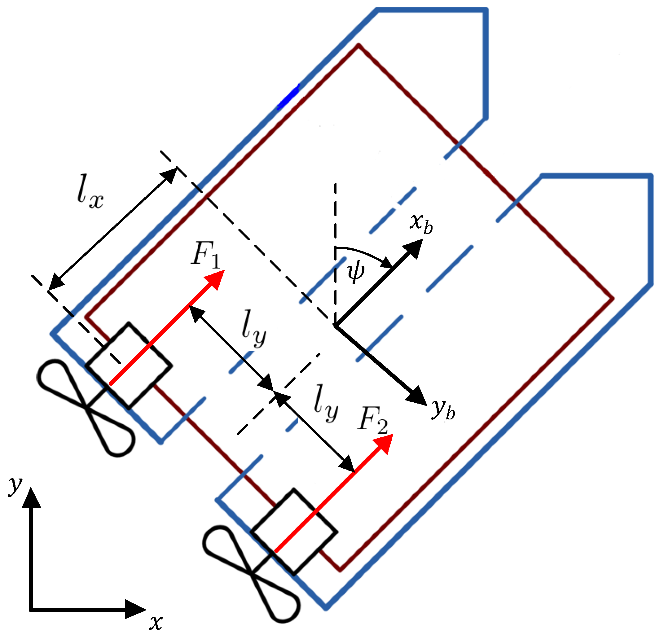
2. Modeling the Dynamics of USVs

The modeling of USVs is briefly discussed in this section as a representative application scenario for which stochastic state estimation schemes are typically applied to reconstruct velocity information and external disturbances by means of measurements of selected state vector components. Typically, these components are the position variables in an earth-fixed coordinate frame that can be determined by means of GPS (global positioning system).

2.1. Dynamic Equations

Throughout this paper, a model with three degrees of freedom (DOF) is used to describe the USV dynamics. It is assumed that in the considered scenario, the motion in terms of roll, pitch, and heave has no significant influence on the maneuvering dynamics of the USV. Therefore, the equations of motion can be written in the form [24,25]

$$\mathit{M}\dot{\mathit{\nu }}+{\mathit{C}}_{RB}\left(\mathit{\nu }\right)\mathit{\nu }+\mathit{N}\left(\mathit{\nu }\right)\mathit{\nu }={\mathit{\tau }}_c.$$

(1)

The translational velocities, expressed in the body-fixed frame in surge and sway, and the rate of rotation in yaw, are expressed by the velocity vector $\mathit{\nu }={\left[\begin{array}{ccc}u& v& r\end{array}\right]}^T$, which represents the velocities (surge and sway velocities and yaw rate) in the three DOF of the system dynamics. The corresponding coordinate systems are shown in Figure 1. The forces in $x_b$ and $y_b$ directions and the moment with respect to the yaw axis provided by the actuators are combined in ${\mathit{\tau }}_c={\left[\begin{array}{ccc}X& Y& N\end{array}\right]}^T$.

The mass matrix

$$\mathit{M}=\left[\begin{array}{ccc}m-X_{\dot{u}}& 0& 0\\ 0& m-Y_{\dot{v}}& m{x}_g-Y_{\dot{r}}\\ 0& m{x}_g-N_{\dot{v}}& J_{zz}-N_{\dot{r}}\end{array}\right]$$

(2)

takes into account the inertia of the rigid body and additional hydrodynamic masses. Coriolis and centripetal terms are summarized in the matrix

$${\mathit{C}}_{RB}=\left[\begin{array}{ccc}0& -mr& -m{x}_{g}r\\ mr& 0& 0\\ m{x}_{g}r& 0& 0\end{array}\right].$$

(3)

The final term

$$\mathit{N}\left(\mathit{\nu }\right)\mathit{\nu }=-\left[\begin{array}{c}-X_{u}u-X_{\left|u\right|u}\left|u\right|u+X_{vr}vr+X_{rr}{r}^2\\ -Y_{v}v-Y_{\left|v\right|v}\left|v\right|v+Y_{ur}ur\\ -N_{r}r-N_{\left|r\right|r}\left|r\right|r+N_{uv}uv+N_{ur}ur\end{array}\right]$$

(4)

on the left-hand side of the dynamic system model (1) accounts for hydrodynamic damping, including coupling effects. For a list of all parameters included in the equations above, and those used in the following subsections, see

Table 1. Description of all parameters used for USV modeling.

Parameter	Description	Unit
m	Displacement	$\mathrm{kg}$
$x_g$	$x^b$-coordinate of center of gravity	$\mathrm{m}$
$J_{comb}$	Moment of inertia w.r.t. the $z^b$ axis (incl. hydrodynamic effects)	${\mathrm{kgm}}^2$
$X_{\dot{u}}$	Hydrodynamic mass in $x^b$-direction	$\mathrm{kg}$
$Y_{\dot{v}}$	Hydrodynamic mass in $y^b$-direction	$\mathrm{kg}$
$Y_{\dot{r}}$	Coupling coefficient of hydrodynamic mass	$\mathrm{kg}·\mathrm{m}$
$N_{\dot{v}}$	Coupling coefficient of hydrodynamic mass	$\mathrm{kg}·\mathrm{m}$
$X_u$	Linear hydrodynamic damping in $x^b$-direction	$\frac{\mathrm{N}}{\mathrm{m}/\mathrm{s}}$
$Y_v$	Linear hydrodynamic damping in $y^b$-direction	$\frac{\mathrm{N}}{\mathrm{m}/\mathrm{s}}$
$N_r$	Linear hydrodynamic damping around $z^b$-axis	$\frac{\mathrm{Nm}}{\mathrm{rad}/\mathrm{s}}$
$X_{vr}$	Coupling coefficient of hydrodynamic damping	$\frac{\mathrm{N}}{(\mathrm{m}/\mathrm{s})(\mathrm{rad}/\mathrm{s})}$
$X_{rr}$	Coupling coefficient of hydrodynamic damping	$\frac{\mathrm{N}}{{(\mathrm{m}/\mathrm{s})}^2}$
$Y_{ur}$	Coupling coefficient of hydrodynamic damping	$\frac{\mathrm{N}}{(\mathrm{m}/\mathrm{s})(\mathrm{rad}/\mathrm{s})}$
$N_{uv}$	Coupling coefficient of hydrodynamic damping	$\frac{\mathrm{Nm}}{{(\mathrm{m}/\mathrm{s})}^2}$
$N_{ur}$	Coupling coefficient of hydrodynamic damping	$\frac{\mathrm{Nm}}{(\mathrm{m}/\mathrm{s})(\mathrm{rad}/\mathrm{s})}$
$X_{\left|u\right|u}$	Quadratic hydrodynamic damping in $x^b$-direction	$\frac{\mathrm{N}}{{(\mathrm{m}/\mathrm{s})}^2}$
$Y_{\left|v\right|v}$	Quadratic hydrodynamic damping in $y^b$-direction	$\frac{\mathrm{N}}{{(\mathrm{m}/\mathrm{s})}^2}$
$N_{\left|r\right|r}$	Quadratic hydrodynamic damping around $z^b$-axis	$\frac{\mathrm{Nm}}{{(\mathrm{rad}/\mathrm{s})}^2}$
$a_1$	Thrust parameter (forward thrust)	−
$b_1$	Thrust parameter (forward thrust and velocity)	−
$a_2$	Thrust parameter (backward thrust)	−
$b_2$	Thrust parameter (backward thrust and velocity)	−

.

2.2. Propulsion

The propulsion system of the USV consists of two fixed jet thrusters arranged in a differential setup (Figure 1). The thrust force of the jet thrusters is described by the expression

$$F_i=c_{1,i}\rho d_p^4{n}_i|n_i|-c_{2,i}\rho d_p^3{u}_{a_i}\left|n_i\right|,i\in \{port,star\},$$

(5)

where $n_i$ is the rotational speed of the respective propeller and $u_{a_i}$ the longitudinal velocity of the corresponding jet thruster through the water. Further, $d_p$ is the diameter of the propeller and $\rho$ the water density. The thrust parameters $c_{1,i}$ and $c_{2,i}$ are assumed to be constant for each operation regime. Four operation regimes are assumed which are defined in terms of the sign of both $n_i$ and $u_{a_i}$. This so-called four-quadrant model is given by

$$\left[\begin{array}{c}{c}_{1,i}\\ c_{2,i}\end{array}\right]=\left\{\begin{array}{cc}{\left[\begin{array}{cc}{a}_{1,i}& b_{1,i}\end{array}\right]}^T& n_i\ge 0\wedge u_{a_i}\ge 0\\ {\left[\begin{array}{cc}{a}_{1,i}& 0\end{array}\right]}^T& n_i\ge 0\wedge u_{a_i}<0\\ {\left[\begin{array}{cc}{a}_{2,i}& 0\end{array}\right]}^T& n_i<0\wedge u_{a_i}\ge 0\\ {\left[\begin{array}{cc}{a}_{2,i}& b_{2,i}\end{array}\right]}^T& n_i<0\wedge u_{a_i}<0\end{array}\right.$$

(6)

with the constant parameters $a_{1,i}$, $a_{2,i}$, $b_{1,i}$, and $b_{2,i}$. For a more detailed discussion on the propulsion model, the reader is referred to [26].

Since the propulsion system is set up differentially, the velocities $u_{a_i}$ are usually different if the USV changes its orientation. With the help of $l_y$, describing the distance between both thrusters, cf. Figure 1, the velocity of the portside thruster ($u_{a_{port}}$) and the velocity of the starboard thuster ($u_{a_{star}}$) are expressed as

$$u_{a_{port}}=u+l_{y}r\mathrm{and}{u}_{a_{star}}=u-l_{y}r$$

(7)

in terms of the velocity u in surge and the yaw rate r.

Finally, the input vector containing the force in the direction of motion and the yaw moment results in

$${\mathit{\tau }}_c=\mathit{T}\left[\begin{array}{c}{F}_{port}\\ F_{star}\end{array}\right]=\mathit{T}\mathit{f}\left(\mathit{u}\right),$$

(8)

with the configuration matrix

$$\mathit{T}=\left[\begin{array}{cc}1& 1\\ 0& 0\\ l_y& -l_y\end{array}\right].$$

(9)

2.3. Parameter Values

As can be seen in Equations (2)–(4) and (6), a total of 22 parameters are included in the model. The number of parameters can be reduced if a specific USV is considered. Here, the overall mass $m=33\mathrm{kg}$ of the USV and the distance $x_g=0$ are assumed to be known a priori. Further, due to the cylindrical shape of the hull of the USV, the commonly used assumption $X_{\dot{u}}=0.05·m$ is made [25]. Due to the additional assumption that the velocity in sway direction is fairly small, the quadratic damping parameter $Y_{\left|v\right|v}$ can be neglected.

The remaining parameters

$$\begin{array}{cc}\hfill {\mathit{\theta }}_1& =(J_{comb},Y_{\dot{r}},N_{\dot{v}},X_u,Y_v,N_r,X_{\left|u\right|u},N_{\left|r\right|r},X_{vr},X_{rr},Y_{ur},N_{uv},N_{ur}),\hfill \\ \hfill {\mathit{\theta }}_2& =(a_1,a_2,b_1),\hfill \end{array}$$

(10)

can be determined by means of numerical optimization with the help of experimental data that are gathered during dedicated driving maneuvers. A further parameter reduction can be performed using sensitivity and correlation analysis. The process of the parameter identification and reduction of the number of parameters to be identified are described in detail for a specific USV in [27]. The parameters obtained during this identification process are listed in

Table 2. Estimated parameters (reduced parameter set).

$J_{comb}$	$X_u$	$Y_v$	$X_{\left|u\right|u}$	$N_{\left|r\right|r}$
$7.20{\mathrm{kgm}}^2$	$-4.62\frac{\mathrm{N}}{\mathrm{m}/\mathrm{s}}$	$-255.26\frac{\mathrm{N}}{\mathrm{m}/\mathrm{s}}$	$-6.53\frac{\mathrm{N}}{{(\mathrm{m}/\mathrm{s})}^2}$	$-9.45\frac{\mathrm{N}}{{(\mathrm{rad}/\mathrm{s})}^2}$
$X_{vr}$	$N_{ur}$	$N_{uv}$	$a_1$	$a_2$
$-129.12\frac{{\mathrm{Ns}}^2}{(\mathrm{m}·\mathrm{rad})}$	$6.67\frac{{\mathrm{Nms}}^2}{(\mathrm{m}·\mathrm{rad})}$	$-48.84\frac{\mathrm{Nm}}{{(\mathrm{m}/\mathrm{s})}^2}$	$0.97$	$0.47$

. Note that all parameters not listed explicitly in the table or in the preceding text are set to zero in the remainder of this article.

2.4. Temporal Discretization and Definition of an Augmented Set of State Equations

To use the dynamic equations of the USV in a discrete-time simulation and state estimation environment with constant sampling period $T_s$, the forward Euler discretization approach is used. The assumption of sufficiently small step sizes, and thus, negligible time discretization errors, leads to the transition equation given by

$${\mathit{x}}_{s,k+1}={\mathit{x}}_{s,k}+T_s{\mathit{f}}_s({\mathit{x}}_{s,k},n_{port,k},n_{star,k})$$

(11)

with the state ${\mathit{x}}_s={\left[\begin{array}{cccccc}x& y& \psi & u& v& r\end{array}\right]}^T$ of the USV and

$${\mathit{f}}_s({\mathit{x}}_s,n_{port},n_{star})=\left[\begin{array}{c}\mathit{J}\mathit{\nu }\\ {\mathit{M}}^{-1}\left({\mathit{\tau }}_c(n_{port},n_{star})-{\mathit{C}}_{RB}\left(\mathit{\nu }\right)\mathit{\nu }-\mathit{N}\left(\mathit{\nu }\right)\mathit{\nu }\right)\end{array}\right]$$

(12)

as the first-order set of state equations, including the kinematic transformation matrix

$$\mathit{J}=\left[\begin{array}{ccc}cos\psi & -sin\psi & 0\\ sin\psi & cos\psi & 0\\ 0& 0& 1\end{array}\right].$$

(13)

In the further course of this work, a total of four parameters of the propulsion system are assumed to be imprecisely known so that they have to be estimated in addition to the USV state by using the available position measurements. Therefore, the state equation is augmented by introducing a four-component integrator disturbance model according to

$$\mathit{f}({\mathit{x}}_s,n_{port},n_{star})=\left[\begin{array}{c}{\mathit{f}}_s({\mathit{x}}_s,n_{port},n_{star})\\ {\mathbf{0}}_{4\times 1}\end{array}\right],$$

(14)

after appending the parameters $p_{1,i}$ and $p_{2,i}$, $i\in \{port,star\}$, to the state vector ${\mathit{x}}_{s,k}$, which allow for replacing the parameters ${\left[\begin{array}{cc}{c}_{1,i}& c_{2,i}\end{array}\right]}^T$ of the four-quadrant model (6) with the multiplicative uncertainty representation ${\left[\begin{array}{cc}{c}_{1,i}·p_{1,i}& c_{2,i}·p_{2,i}\end{array}\right]}^T$.

2.5. Measurement Model

For the state estimation, the absolute position coordinates x and y are measured in the earth-fixed coordinate frame, for example, by using GPS. Since both values are assumed to be affected by zero-mean white Gaussian noise, the measurement model is given by

$$\begin{array}{cc}\hfill z_x& =x+w_1\hfill \\ \hfill z_y& =y+w_2,\hfill \end{array}$$

(15)

where $w_i\sim \mathcal{N}(w_i;0,\sigma )$ with the coordinate-independent scalar standard deviation $\sigma$.

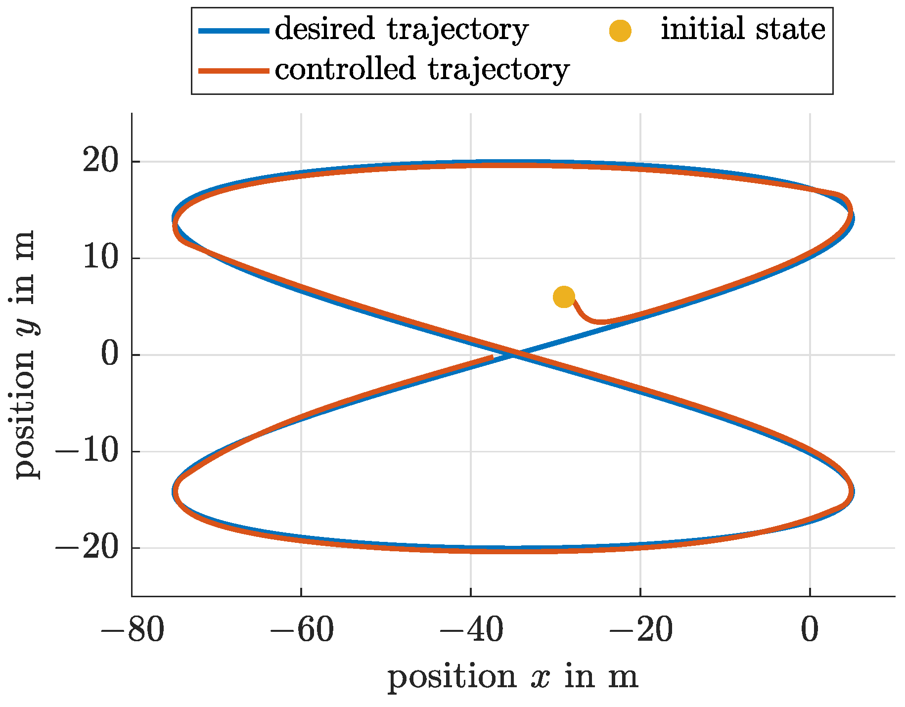
2.6. Tracking Control Using an Artificial Potential Field Approach

The tracking controller based on an artificial potential field approach [28,29,30] was taken from [31]. The approach is described below for completeness. In general, the artificial potential field method has its foundations in the area of robotics. There, it was originally developed as a tool for path and motion planning. In the artificial potential field approach, attracting potentials are introduced for the target states to be reached, and repelling potentials are employed to avoid collisions with obstacles. The references mentioned above represent generalizations of this approach for control purposes, especially with respect to the definition of an attracting potential for the desired trajectory that is to be tracked by the controller.

The control law is given by

$${\tilde{F}}_{d,i}=(K_0-K_{P,i}(arg\left(\mathit{\omega }\right)-\psi )+K_{D,i}\dot{\psi }){\omega }^2,i\in \{port,star\},$$

(16)

where the desired thrust levels ${\tilde{F}}_{d,i}$ of the portside and starboard propellers ($i\in \{port,star\}$) are saturated to only forward thrusts up to $F_{d,max}$, using the relation

$$F_{d,i}=\left\{\begin{array}{ccc}0& \mathrm{if}& {\tilde{F}}_{d,i}\le 0\\ F_{d,max}& \mathrm{if}& {\tilde{F}}_{d,i}\ge F_{d,max}\\ {\tilde{F}}_{d,i}& \mathrm{else}.& \end{array}\right.$$

(17)

The gains in (16) were experimentally tuned and satisfy the relations

$$K_0>0,K_{P,port}=-K_{P,star}\mathrm{and}{K}_{D,port}=-K_{D,star}.$$

(18)

The amplitude $\omega$ in (16) is the Euclidian vector norm $\omega =\parallel \mathit{w}\parallel$ of the input vector

$$\mathit{w}=\gamma \parallel {\dot{\mathit{y}}}_d\parallel ({\mathit{y}}_d-\mathit{y})+{\dot{\mathit{y}}}_d$$

(19)

depending on the earth-fixed position vector of the USV $\mathit{y}={\left(\begin{array}{cc}x& y\end{array}\right)}^T$, the desired position vector ${\mathit{y}}_d$, the desired velocity vector ${\dot{\mathit{y}}}_d$, and the tuning parameter $\gamma$. Finally, to obtain the desired speeds of the propellers, Equation (5) needs to be inverted using the desired thrusts from the controller. Since $b_1$ and $b_2$ are zero and only positive thrusts are allowed (cf. (17)), the rotational speed of the propellers can be calculated using the relation

$$n_i=\sqrt{\frac{F_i}{c_1\rho d_p^4}},i\in \{port,star\}.$$

(20)

3. UKF State Estimation

The nonlinear ship model presented in Section 2 is used in combination with the linear measurement model (15) to perform a model-based reconstruction of velocity information and to reconstruct the multiplicative parameter uncertainty, mentioned in the previous section. To deal with the corresponding nonlinearities, a UKF state prediction [12,14] is used, and for the update step, a linear Kalman filter update is sufficient.

It is assumed that the posterior is given as a Gaussian with mean ${\mathit{x}}_{k-1|k-1}$ and covariance matrix ${\mathit{P}}_{k-1|k-1}$. Since the number of elements of the augmented state is $n=10$ (including the multiplicative disturbance parameters; cf. Equation (14)), a total number of $2n+1=21$ sigma points are used for the prediction. The sigma points are calculated as follows [14] (p. 155):

$$\begin{array}{c}\hfill \begin{array}{cc}{\mathcal{X}}_0={\mathit{x}}_{k-1|k-1},\hfill & \\ {\mathcal{X}}_i={\mathit{x}}_{k-1|k-1}+{\left(\sqrt{(n+\lambda ){\mathit{P}}_{k|k}}\right)}_i^T\hfill & i=1,\dots ,n,\hfill \\ {\mathcal{X}}_i={\mathit{x}}_{k-1|k-1}-{\left(\sqrt{(n+\lambda ){\mathit{P}}_{k|k}}\right)}_{i-n}^T\hfill & i=n+1,\dots ,2n,\hfill \end{array}\end{array}$$

(21)

with the scaling parameters $\lambda$ and ${\left(\sqrt{(n+\lambda ){\mathit{P}}_{k|k}}\right)}_i$ as the ith row of the matrix square root [14] (p. 155). In addition, each sigma point has a corresponding weight. The weights are given by [14] (p. 155):

$$\begin{array}{c}\hfill \begin{array}{cc}{W}_0^{\left(m\right)}={\displaystyle \frac{\lambda }{n+\lambda }},\hfill & \\ W_0^{\left(c\right)}={\displaystyle \frac{\lambda }{n+\lambda }}+(1-{\alpha }^2+\beta ),\hfill & \\ W_i^{\left(m\right)}=W_i^{\left(c\right)}={\displaystyle \frac{1}{2(n+\lambda )}}\hfill & i=1,\dots ,2n,\hfill \end{array}\end{array}$$

(22)

with $\lambda ={\alpha }^2(n+\kappa )-n$. For the tuning parameters, we chose $\alpha =0.01$, $\beta =3$, and $\kappa =0$. A detailed explanation of the tuning parameters is given in [14] (p. 155).

Following the generation of these sigma points in each discretization step, they can be predicted using the nonlinear transition equation

$${\mathcal{Y}}_i={\mathcal{X}}_i+T_s\mathit{f}\left({\mathcal{X}}_i\right)$$

(23)

corresponding to the augmented discrete-time system model that includes the expression (14). Afterwards, the set of sigma points is used to approximate the true probability density by a Gaussian with mean

$$\begin{array}{c}\hfill {\mathit{x}}_{k|k-1}\approx \sum _{i=0}^{2n}{W}_i^{\left(m\right)}{\mathcal{Y}}_i\end{array}$$

(24)

and covariance

$$\begin{array}{c}\hfill {\mathit{P}}_{k|k-1}\approx \sum _{i=0}^{2n}{W}_i^{\left(c\right)}\left({\mathcal{Y}}_i-{\mathit{x}}_{k|k-1}\right){\left({\mathcal{Y}}_i-{\mathit{x}}_{k|k-1}\right)}^T+{\mathit{Q}}_k.\end{array}$$

(25)

As the measurement model (15) is linear with additive Gaussian noise, the measurement errors are Gaussian as well. Thus, the standard Kalman filter update

$$\begin{array}{cc}\hfill {\mathit{z}}_{k|k-1}& ={\mathit{H}}_k{\mathit{x}}_{k|k-1},\hfill \end{array}$$

(26)

$$\begin{array}{cc}\hfill {\mathit{S}}_{k|k-1}& ={\mathit{H}}_k{\mathit{P}}_{k|k-1}{\mathit{H}}_k^T+{\mathit{R}}_k,\hfill \end{array}$$

(27)

$$\begin{array}{cc}\hfill {\mathit{K}}_k& ={\mathit{P}}_{k|k-1}{\mathit{H}}_k^T{\mathit{S}}_{k|k-1}^{-1},\hfill \end{array}$$

(28)

$$\begin{array}{cc}\hfill {\mathit{x}}_{k|k}& ={\mathit{x}}_{k|k-1}+{\mathit{K}}_k\left({\mathit{z}}_k-{\mathit{z}}_{k|k-1}\right),\hfill \end{array}$$

(29)

$$\begin{array}{cc}\hfill {\mathit{P}}_{k|k}& ={\mathit{P}}_{k|k-1}-{\mathit{K}}_k{\mathit{H}}_k{\mathit{P}}_{k|k-1}\hfill \end{array}$$

(30)

can be used to evaluate the innovation step as soon as measured data are available at the time instant k.

4. Ellipsoidal Enclosure Approach for Bounding Confidence Regions

Set-valued simulation and estimation techniques provide the possibility to propagate bounded domains of possible state variables over time through a dynamic system model and to fuse those propagated domains with domains that are compatible with measured information by using set-based intersection operations. A possible implementation of this kind of estimation scheme is given by the tube arithmetic approach detailed in [32,33]. To obtain bounds that contain all reachable domains in the state space with certainty, it is necessary that uncertain system parameters, initial conditions, and external disturbances are bounded by appropriate domains, such as intervals, zonotopes, polytopes, or ellipsoids [34,35,36,37].

To bridge the gap between stochastic and purely set-valued estimation schemes, it was shown in [22] that ellipsoidal estimation approaches can also be used to analyze the reliability of linearization-based stochastic estimators (such as the Extended Kalman Filter) and to compute outer bounds of confidence regions of a certain probability if uncertain state information is described by means of normally distributed probability density functions.

This approach, discussed in [22] for the state prediction, is extended in the following to obtain a complete filter approach that comprises also an innovation stage in which results with a specific confidence level are computed.

4.1. Ellipsoidal Prediction of Confidence Bounds

To use the ellipsoidal calculus approach from [22,38] for the prediction of covariance matrix bounds, assume a discrete-time state-space model

$${\mathbf{z}}_{k+1}=\mathsf{\Phi }\left({\mathbf{z}}_k,\mathbf{p}\right)·{\mathbf{z}}_k+{\mathbf{w}}_k.$$

(31)

In this model, the dynamics matrix $\mathsf{\Phi }\left({\mathbf{z}}_k,\mathbf{p}\right)$ may depend on the state vector ${\mathbf{z}}_k$ and on a bounded parameter vector $\mathbf{p}\in \left[\underset{¯}{\mathbf{p}};\overline{\mathbf{p}}\right]$ with the elementwise defined relation $\underset{¯}{\mathbf{p}}\le \overline{\mathbf{p}}$. The additive offset term ${\mathbf{w}}_k$ is assumed to represent the influence of bounded external disturbances and control signals that are not directly included (in terms of a closed-loop system model) in the first summand of (31). Throughout this paper, it is assumed that the term ${\mathbf{w}}_k$ is bounded by an ellipsoid. Suitable strategies to obtain these bounds are based on the so-called Löwner–John ellipsoids [39], which can be computed by means of either linear matrix inequalities or enclosed conservatively by using interval arithmetic, as described in Section 4.3 of [33].

We define further an ellipsoidal domain [23]

$${\mathcal{E}}_k\left({\mathit{\mu }}_k,{\tilde{\mathsf{\Gamma }}}_k,r\right):=\left\{{\mathbf{z}}_k\in {\mathbb{R}}^n|{\left({\mathbf{z}}_k-{\mathit{\mu }}_k\right)}^T{\tilde{\mathsf{\Gamma }}}_k^{-T}{\tilde{\mathsf{\Gamma }}}_k^{-1}\left({\mathbf{z}}_k-{\mathit{\mu }}_k\right)\le r^2\right\}$$

(32)

with the positive definite shape matrix ${\tilde{\mathbf{Q}}}_k={\tilde{\mathsf{\Gamma }}}_k{\tilde{\mathsf{\Gamma }}}_k^T\succ 0$ and the ellipsoid midpoint ${\mathit{\mu }}_k\in {\mathbb{R}}^n$. When compared with a stochastic state prediction algorithm, the midpoint vector ${\mathit{\mu }}_k$ can be interpreted as the mean of the corresponding probability density.

The parameter r describes a magnification factor according to [40] so that the ellipsoid (32) specifies the confidence bound of a given percentage if the vector ${\mathbf{z}}_k$ is normally distributed with the covariance ${\tilde{\mathbf{Q}}}_k$. For a list of specific values of this magnification factor for dimensions $n\le 10$, the reader is referred to [40].

For compact notation of the following ellipsoidal covariance prediction step, define the matrices

$${\mathsf{\Gamma }}_k:=r·{\tilde{\mathsf{\Gamma }}}_k\mathrm{and}{\mathbf{Q}}_k:=r^2·{\tilde{\mathbf{Q}}}_k.$$

(33)

The following procedure is based on reference [38], from which only the computation of outer ellipsoidal bounds is taken into consideration.

For the compactness of notation, reformulate the summand $\mathsf{\Phi }\left({\mathbf{z}}_k,\mathbf{p}\right)·{\mathbf{z}}_k$ in the system model (31) into the form

$$\mathsf{\Phi }\left({\mathbf{z}}_k,\mathbf{p}\right)·{\mathbf{z}}_k=\mathsf{\Phi }\left({\mathbf{z}}_k,\mathbf{p}\right)·{\check{\mathbf{z}}}_k+\tilde{\mathsf{\Phi }}·{\mathit{\mu }}_k+\left(\mathsf{\Phi }\left({\mathbf{z}}_k,\mathbf{p}\right)-\tilde{\mathsf{\Phi }}\right)·{\mathit{\mu }}_k$$

(34)

with ${\mathbf{z}}_k={\check{\mathbf{z}}}_k+{\mathit{\mu }}_k$, where

$${\mathbf{z}}_k\in {\mathcal{E}}_k={\mathcal{E}}_k\left({\mathit{\mu }}_k,{\tilde{\mathsf{\Gamma }}}_k,r\right).$$

(35)

Here, ${\mathcal{E}}_k$ denotes the uncertainty on the non-origin centered states ${\mathbf{z}}_k$,

$${\check{\mathbf{z}}}_k\in {\check{\mathcal{E}}}_k={\check{\mathcal{E}}}_k\left(\mathbf{0},{\tilde{\mathsf{\Gamma }}}_k,r\right)$$

(36)

the uncertainty on ${\check{\mathbf{z}}}_k$ after shifting the ellipsoid to the origin, and

$$\tilde{\mathsf{\Phi }}=\mathsf{\Phi }\left({\mathit{\mu }}_k,\mathrm{mid}\left(\left[\mathbf{p}\right]\right)\right)$$

(37)

is the midpoint approximation of the quasi-linear system matrix with

$$\mathrm{mid}\left(\left[\mathbf{p}\right]\right)=\frac{1}{2}·\left(\underset{¯}{\mathbf{p}}+\overline{\mathbf{p}}\right).$$

(38)

Let $\square {\mathcal{E}}_k$ denote an axis-aligned enclosure of ${\mathcal{E}}_k$ in the form of an interval box in the coordinate frame ${\mathbf{z}}_k$.

Considering the term $\mathsf{\Phi }\left({\mathbf{z}}_k,\mathbf{p}\right)·{\mathbf{z}}_k$, a guaranteed outer confidence bound of magnification r is given for this summand by the ellipsoid ${\mathcal{E}}_{\mathsf{\Phi },k+1}\left({\mathit{\mu }}_{k+1},{\tilde{\mathsf{\Gamma }}}_{k+1},r\right)$ with the covariance

$${\tilde{\mathbf{Q}}}_{\mathsf{\Phi },k+1}={\tilde{\mathsf{\Gamma }}}_{\mathsf{\Phi },k+1}{\left({\tilde{\mathsf{\Gamma }}}_{\mathsf{\Phi },k+1}\right)}^T$$

(39)

according to the following steps. This procedure is given without further proof because it is a direct consequence of the work published in [38].

P1:

Apply

$${\check{\mathbf{z}}}_{k+1}=\mathsf{\Phi }\left({\mathbf{z}}_k,\mathbf{p}\right)·{\check{\mathbf{z}}}_k$$

(40)

to the ellipsoid ${\check{\mathcal{E}}}_k$ in (36). The outer ellipsoid enclosure of the image set is described by an ellipsoid with the shape matrix

$${\check{\mathbf{Q}}}_{k+1}={\alpha }_{k+1}^2·{\mathsf{\Gamma }}_{k+1}·{\mathsf{\Gamma }}_{k+1}^T,$$

(41)

where ${\alpha }_{k+1}\ge 0$ is the smallest value for which the LMI

$${\mathcal{M}}_{k+1}:=\mathsf{\Lambda }\left[\begin{array}{cc}-{\mathbf{Q}}_k^{-1}& {\mathsf{\Phi }}^T\left({\mathbf{z}}_k,\mathbf{p}\right)·{\tilde{\mathsf{\Phi }}}^{-T}\\ {\tilde{\mathsf{\Phi }}}^{-1}·\mathsf{\Phi }\left({\mathbf{z}}_k,\mathbf{p}\right)& -{\alpha }_{k+1}^2{\mathcal{R}}_k\end{array}\right]\mathsf{\Lambda }⪯0$$

(42)

is satisfied for all ${\mathbf{z}}_k\in \square {\mathcal{E}}_k$, i.e., for all state realizations in the interior of an axis-aligned tight enclosure of the ellipsoid, and for all possible parameters $\mathbf{p}\in \left[\mathbf{p}\right]$ with the shape matrix parameterization

$${\mathcal{R}}_k:={\mathsf{\Gamma }}_k·{\mathsf{\Gamma }}_k^T.$$

(43)

In (42), the symbol ⪯ denotes the negative semi-definiteness of the corresponding matrix expression. For possible strategies to select the preconditioning matrix $\mathsf{\Lambda }$, aiming at a reduction of pessimism when computing this guaranteed outer ellipsoid enclosure, see [33].

P2:

Compute interval bounds for the term

$${\mathbf{b}}_k=\left(\mathsf{\Phi }\left(\mathbf{p}\right)-\tilde{\mathsf{\Phi }}\right)·{\mathit{\mu }}_k\in \left[{\mathbf{b}}_k\right]$$

(44)

which accounts for a non-zero ellipsoid midpoint with ${\mathbf{z}}_k$, $\tilde{\mathsf{\Phi }}$, and $\mathbf{p}$ defined according to (35), (37), and (38). Inflate the ellipsoid bound described by the shape matrix (41) according to

$$\begin{array}{cc}\hfill {\mathbf{Q}}_{\mathsf{\Phi },k+1}& ={\left(1+{\rho }_{\mathrm{O},k+1}\right)}^2·{\check{\mathbf{Q}}}_{k+1},\hfill \end{array}$$

(45)

$$\begin{array}{cc}\hfill {\rho }_{\mathrm{O},k+1}& =sup\left\{∥{\alpha }_{k+1}^{-1}·{\mathsf{\Gamma }}_k^{-1}·\left[{\mathbf{b}}_k\right]∥\right\},\hfill \end{array}$$

(46)

where the interval-valued generalization of the Euclidean norm operator in (46) is defined in [22].

P3:

Compute the updated ellipsoid midpoint

$${\mathit{\mu }}_{\mathsf{\Phi },k+1}=\tilde{\mathsf{\Phi }}·{\mathit{\mu }}_k$$

(47)

and the updated square root of its shape matrix

$$\begin{array}{c}\hfill {\tilde{\mathsf{\Gamma }}}_{\mathsf{\Phi },k+1}={\alpha }_{k+1}·\left(1+{\rho }_{\mathrm{O},k+1}\right)·\tilde{\mathsf{\Phi }}·{\tilde{\mathsf{\Gamma }}}_k.\end{array}$$

(48)

P4:

Compute an ellipsoidal enclosure of the Minkowski sum of the ellipsoid ${\mathcal{E}}_{\mathsf{\Phi },k+1}$ and the ellipsoid ${\mathcal{E}}_{\mathbf{w},k}={\mathcal{E}}_k\left({\mathit{\mu }}_{\mathbf{w},k},{\tilde{\mathsf{\Gamma }}}_{\mathbf{w},k},r_{\mathbf{w}}\right)$ enclosing the term ${\mathbf{w}}_k$ according to

$${\mathcal{E}}_{\mathsf{\Phi },k+1}\oplus {\mathcal{E}}_{\mathbf{w},k}\subseteq {\mathcal{E}}_{k+1}\left({\mathit{\mu }}_{k+1},{\mathsf{\Gamma }}_{k+1},r\right)$$

(49)

with the new midpoint

$${\mathit{\mu }}_{k+1}={\mathit{\mu }}_{\mathsf{\Phi },k+1}+{\mathit{\mu }}_{\mathbf{w},k}$$

(50)

and the updated square root of the shape matrix (resp., square root of the new covariance matrix)

$${\tilde{\mathsf{\Gamma }}}_{k+1}={\left({\tilde{\mathbf{Q}}}_{k+1}\right)}^{\frac{1}{2}},$$

(51)

which is given in closed-form by the nearly optimal shape matrix (i.e., close to the minimum volume ellipsoid)

$${\tilde{\mathbf{Q}}}_{k+1}=\frac{1}{r^2}\left(r^2·\left(1+\frac{1}{\beta }\right)·\left({\mathsf{\Gamma }}_{\mathsf{\Phi },k+1}·{\mathsf{\Gamma }}_{\mathsf{\Phi },k+1}^T\right)+r_{\mathbf{w}}^2·\left(1+\beta \right)·\left({\mathsf{\Gamma }}_{\mathsf{\Psi },k+1}·{\mathsf{\Gamma }}_{\mathsf{\Psi },k+1}^T\right)\right)$$

(52)

with

$$\beta =\sqrt{\frac{\mathrm{trace}\left\{{\mathsf{\Gamma }}_{\mathsf{\Phi },k+1}·{\mathsf{\Gamma }}_{\mathsf{\Phi },k+1}^T\right\}}{\mathrm{trace}\left\{{\mathsf{\Gamma }}_{\mathsf{\Psi },k+1}·{\mathsf{\Gamma }}_{\mathsf{\Psi },k+1}^T\right\}}}.$$

(53)

For a derivation of this expression, the reader is referred to [37,41,42].

4.2. Ellipsoidal Innovation Stage with Predefined Confidence Bounds

To perform the intersection of ellipsoids that represent the predicted state domains derived in the previous section and (possibly degenerate) ellipsoids that enclose all states compatible with the measured data, where each of them accounts for a user-defined confidence level, the procedure published in Section 4.2 of [33] is used without any modification. In contrast to widely known approaches from the literature, it is a generalization which allows for not only intersecting ellipsoids with identical midpoints but also for enclosing the intersections of ellipsoids with different midpoints. One of those ellipsoids may be infinitely wide in some dimensions of the state space for which no measured information exists.

For that purpose, the following two steps introduced in Section 4.2 of [33] are employed:

C1:

Determine the common midpoint for the desired outer bound of the intersection that must be included in all ellipsoids to be intersected (after the ellipsoid widening operations according to Equations (51) and (52) of [33]);

C2:

Determine the shape matrices for the outer ellipsoid bound according to the computation of Dikin ellipsoids according to [43].

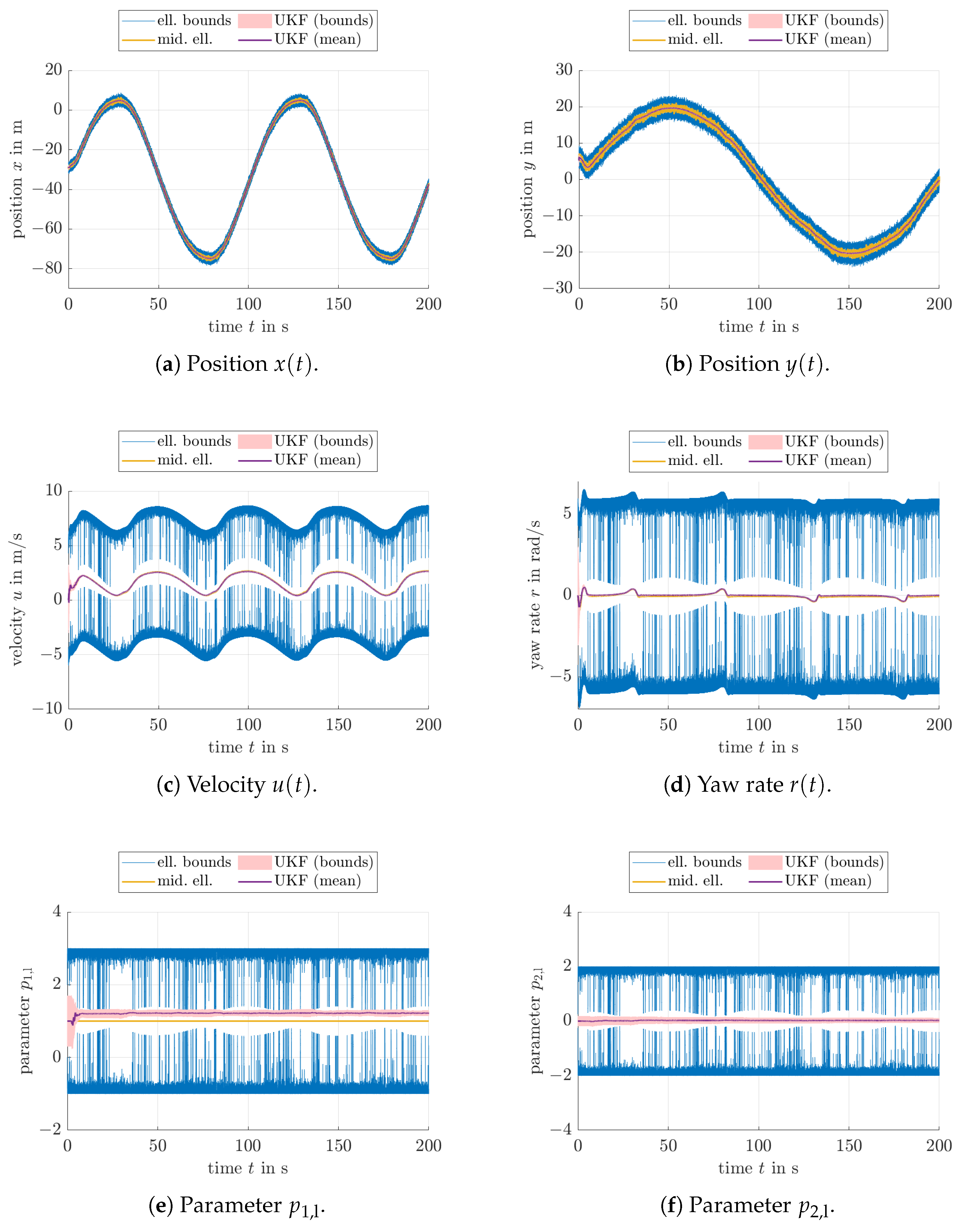
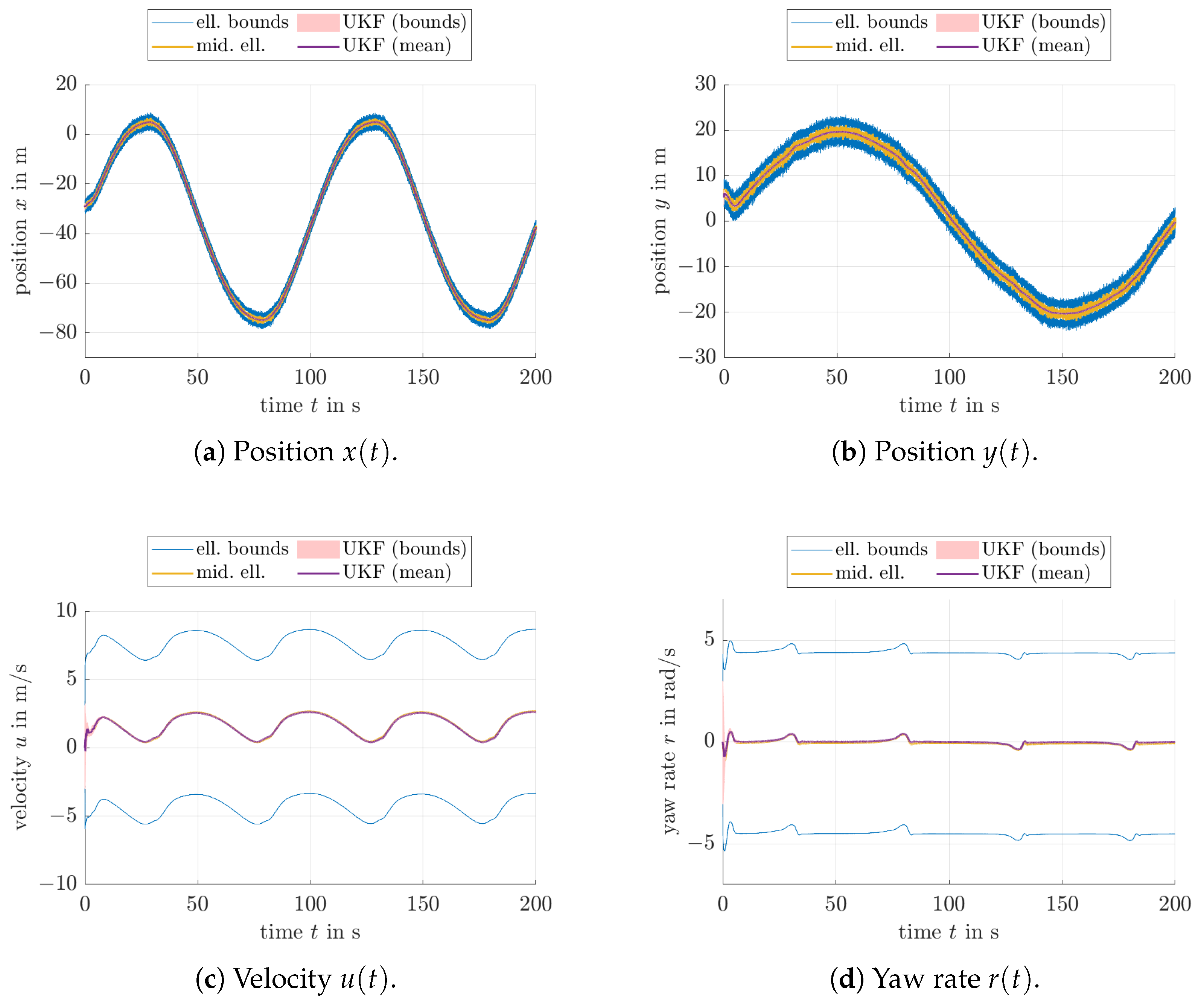
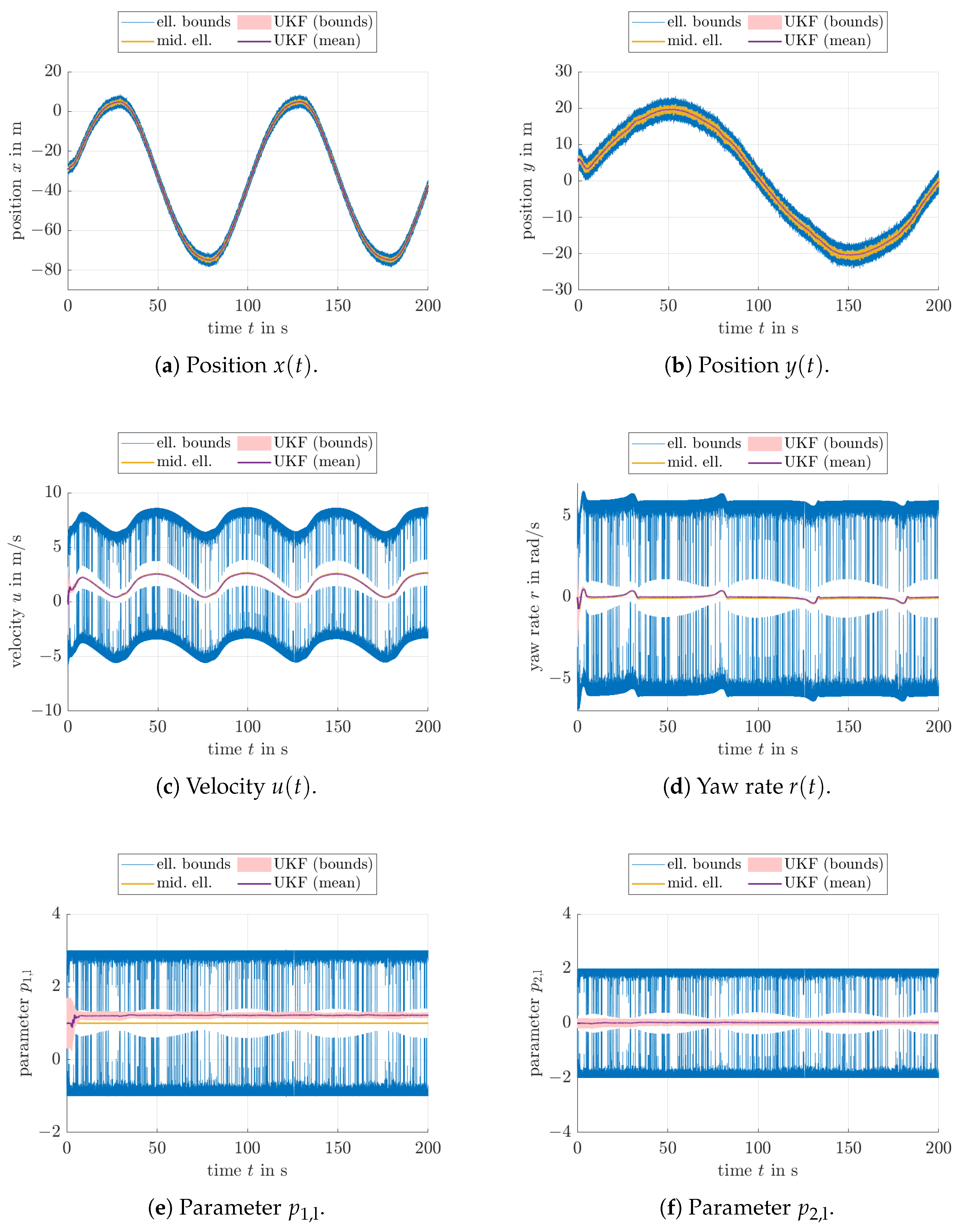
5. Simulation Results

To perform the reliability assessment of the UKF approach by means of the proposed ellipsoidal enclosure approach, assume that the additive process noise is parameterized by the purely diagonal covariance matrix

$$\mathit{Q}=\mathrm{diag}\left\{\left[\begin{array}{cccccccccc}0& 0& 0& 0.25& 0.25& 0.0076& 0.25& 0.25& 0.01& 0.01\end{array}\right]\right\}·{10}^{-6}$$

(54)

and the position measurement covariance by

$$\mathit{R}=\mathrm{diag}\left\{\left[\begin{array}{cc}0.25& 0.25\end{array}\right]\right\}.$$

(55)

Moreover, the initial mean of the Gaussian probability density describing the uncertainty in the state vector to be estimated is chosen as

$$x_0={\left[\begin{array}{cccccccccc}{z}_{x,0}& z_{y,0}& 0& 0& 0& 0& 1& 1& 0& 0\end{array}\right]}^T$$

(56)

with $z_{x,0}\approx -29.14\mathrm{m}$ and $z_{y,0}\approx 4.99\mathrm{m}$, resulting from randomly disturbing the true initial vessel position $(-29\mathrm{m};5\mathrm{m})$, which has an offset of $6\mathrm{m}$ in each coordinate in comparison with the desired initial state, according to the initial state covariance (augmented by the integrator disturbance states according to Equation (14))

$${\mathit{P}}_0=\mathrm{diag}\left\{\left[\begin{array}{cccccccccc}0.25& 0.25& 1& 1& 1& 1& 0.0535& 0.0535& 0.0033& 0.0033\end{array}\right]\right\}.$$

(57)

The desired vessel trajectory, serving as a reference for the artificial potential field controller, and the trajectory of the controlled ship motion, are illustrated in Figure 2.

All continuous-time state equations have been discretized in this section by using an explicit Euler scheme with a constant sampling period of $10\mathrm{ms}$, corresponding also to the sampling time of the available position measurements.

For the reliability assessment in Figure 3, Figure 4 and Figure 5, it has been assumed that the ellipsoidal enclosure technique is parameterized with scaling factors that represent 99% confidence bounds for both the process and measurement noise in all cases under consideration. For a list of the corresponding scaling factors, deduced by a computationally efficient recursion formula that is based on a ${\chi }^2$ distribution with the state dimension as degrees of freedom, the reader is referred to [40].

In addition, the scaling factor r representing the minimum coverage of the expected state according to [23] was varied in all depicted simulations. The first simulation in Figure 3 assumed constant bounds for the uncertain system parameters that are introduced by means of the integrator disturbance models mentioned above and in Equation (14), and the UKF simultaneously estimated these values at run-time. The interior of the non-rescaled ellipsoids with $r=1$ leads to a confidence level of $1.44\%$ due to the state dimension $n=6$; cf. [40].

A comparison of Figure 3 with Figure 4 and Figure 5 indicates that the enhanced parameter bounds—obtained in the ellipsoidal evaluation when using the augmented system model there as well—provide much tighter estimates for the velocity and yaw rate information (indicated in blue color) than in the case of uncertain but bounded parameters. The visible chattering of the respective bounds in Figure 4c,d and Figure 5c,d is caused by the fact that the ellipsoidal estimator is a priori initialized with the worst-case outer bound on the possible parameters and that intersections of the estimated domains resulting from the prediction step may significantly be inflated if the corresponding parameter ellipsoid midpoints deviate strongly from the ellipsoid information obtained in the set-valued innovation step; cf. [38].

However, the advantage of this behavior is the fact that the computed bounds always represent guaranteed outer enclosures of the reachable state domains with the confidence levels r that have been specified. This statement holds true even despite nonlinearities in the underlying dynamic system model. Future work can address an enhancement of the associated model for parameter variations in such a way that the general idea of a forgetting factor-like approach [44] will be transferred to set-valued online parameter estimation techniques. Such approaches will then be used also to limit the temporal parameter variation rates between two subsequent sampling instants of the ellipsoidal estimator to a user-defined rate.

However, for the application at hand, it can be seen that the computed ellipsoid bounds, especially in Figure 5, practically always bound the 3-standard deviation ranges determined by means of the UKF from the outside. This behavior helps to confirm that the UKF produces state estimates that do not violate the ellipsoidal bounds with the identical confidence level due to, for example, biased state estimates that would be caused by a large influence of linearization errors or by a convergence to an ambiguous state in the case of probability densities that may have a multi-modal shape (in fact, such scenarios can even exist in the model at hand if the heading uncertainty becomes so large that forward and backward motion could no longer be distinguished). In addition, it becomes obvious that the most crucial factor reducing the sensitivity of velocity, and therefore, also position estimates is the accurate online identification of the disturbance parameters that are associated with the uncertain model for the USV’s propulsion system. For that reason, especially those parameters need to be identified accurately (possibly at run-time) in order to achieve not only reliable state estimates but also to obtain accurate trajectory tracking capabilities if either the proposed UKF-based estimator or the ellipsoidal counterpart is included in a closed-loop or predictive control structure. However, it should be pointed out that especially for the velocity estimates, the UKF-based uncertainty ranges are much tighter than the set-valued counterparts. This gives rise to the assumption that the UKF performs strong smoothing of the estimated values, but delivers uncertainty bounds that may be more optimistic than they would actually be in reality.

6. Conclusions and Outlook on Future Work

In this paper, a stochastic interpretation of an ellipsoidal state estimation procedure has been introduced and applied to the reliability assessment of a UKF-based state estimation for USVs which is purely based on position measurements. It has been shown that this approach allows for checking whether the Gaussian assumption made by a UKF leads to estimates that are explainable also by performing set-valued prediction and innovation stages that cover the identical confidence bounds.

Future work will address the experimental validation of the proposed ellipsoidal enclosure techniques, for example, by using the DDboat robots presented in [31]. Moreover, methodological developments will focus on the case of mixed uncertainty models (e.g., by describing measurement uncertainty by Gaussian probabilities and parameter uncertainty with the help of set-valued counterparts). First attempts into this direction have already been made in [23], where a stochastic approach for iterative learning observer design was investigated recently. Moreover, interfaces between such mixed uncertainty representations in state estimation algorithms and predictive control procedures will be a further subject of future work.

References

1. Maybeck, P.S. Stochastic Models, Estimation, and Control, Volume 1; Academic Press, Inc.: New York, NY, USA, 1979. [Google Scholar]
2. Maybeck, P.S. Stochastic Models, Estimation, and Control, Volume 2; Academic Press, Inc.: New York, NY, USA, 1982. [Google Scholar]
3. Maybeck, P.S. Stochastic Models, Estimation, and Control, Volume 3; Academic Press, Inc.: New York, NY, USA, 1982. [Google Scholar]
4. Anderson, B.D.O.; Moore, J.B. Optimal Filtering; Dover Publications, Inc.: Mineola, NY, USA, 2005. [Google Scholar]
5. Papoulis, A. Probability, Random Variables, and Stochastic Processes; McGraw-Hill: New York, NY, USA, 1991. [Google Scholar]
6. Stengel, R. Optimal Control and Estimation; Dover Publications, Inc.: Mineola, NY, USA, 1994. [Google Scholar]
7. Åström, K.J. Introduction to Stochastic Control Theory; Mathematics in Science and Engineering; Academic Press: New York, NY, USA, 1970. [Google Scholar]
8. Hermann, R.; Krener, A.J. Nonlinear Controllability and Observability. IEEE Trans. Autom. Control 1977, 22, 728–740. [Google Scholar] [CrossRef] [Green Version]
9. Sontag, E. Mathematical Control Theory—Deterministic Finite Dimensional Systems; Springer: New York, NY, USA, 1998. [Google Scholar]
10. Kalman, R.E. A New Approach to Linear Filtering and Prediction Problems. Trans. ASME-J. Basic Eng. 1960, 82, 35–45. [Google Scholar] [CrossRef] [Green Version]
11. Daum, F. Nonlinear Filters: Beyond the Kalman Filter. IEEE Aerosp. Electron. Syst. Mag. 2005, 20, 57–69. [Google Scholar] [CrossRef]
12. Julier, S.J.; Uhlmann, J.K.; Durrant-Whyte, H.F. A New Approach for the Nonlinear Transformation of Means and Covariances in Filters and Estimators. IEEE Trans. Autom. Control 2000, 45, 477–482. [Google Scholar] [CrossRef] [Green Version]
13. Uhlmann, J.K. First-Hand: The Unscented Transform. Available online: https://ethw.org/First-Hand:The_Unscented_Transform (accessed on 26 June 2022).
14. Wan, E.A.; Van Der Merwe, R. The Unscented Kalman Filter for Nonlinear Estimation. In Proceedings of the IEEE 2000 Adaptive Systems for Signal Processing, Communications, and Control Symposium (Cat. No. 00EX373), Lake Louise, AB, Canada, 4 October 2000; pp. 153–158. [Google Scholar]
15. Sorenson, H.W.; Alspach, D.L. Recursive Bayesian Estimation Using Gaussian Sums. Automatica 1971, 7, 465–479. [Google Scholar] [CrossRef]
16. Alspach, D.; Sorenson, H. Nonlinear Bayesian Estimation Using Gaussian Sum Approximations. IEEE Trans. Autom. Control 1972, 17, 439–448. [Google Scholar] [CrossRef]
17. Terejanu, G.; Singla, P.; Singh, T.; Scott, P.D. Adaptive Gaussian Sum Filter for Nonlinear Bayesian Estimation. IEEE Trans. Autom. Control 2011, 56, 2151–2156. [Google Scholar] [CrossRef]
18. Rauh, A.; Briechle, K.; Hanebeck, U.D. Nonlinear Measurement Update and Prediction: Prior Density Splitting Mixture Estimator. In Proceedings of the 2009 IEEE Control Applications, (CCA) & Intelligent Control, (ISIC), St. Petersburg, Russia, 8–10 July 2009. [Google Scholar]
19. Del Moral, P. Non Linear Filtering: Interacting Particle Solution. Markov Process. Relat. Fields 1996, 2, 555–580. [Google Scholar]
20. Dekhici, B.; Benyahiya, B.; Cherki, B. Forecast of Chemostat Dynamics Using Data-Driven Approach. In Proceedings of the 2021 International Conference on Control, Automation and Diagnosis (ICCAD), Grenoble, France, 3–5 November 2021; pp. 1–6. [Google Scholar] [CrossRef]
21. Koopman, B.O.; Neumann, J.V. Dynamical Systems of Continuous Spectra. Proc. Natl. Acad. Sci. USA 1932, 18, 255–263. [Google Scholar] [CrossRef] [Green Version]
22. Rauh, A.; Jaulin, L. A Computationally Inexpensive Algorithm for Determining Outer and Inner Enclosures of Nonlinear Mappings of Ellipsoidal Domains. Int. J. Appl. Math. Comput. Sci. AMCS 2021, 31, 399–415. [Google Scholar]
23. Rauh, A.; Chevet, T.; Dinh, T.N.; Marzat, J.; Raïssi, T. Robust Iterative Learning Observers Based on a Combination of Stochastic Estimation Schemes and Ellipsoidal Calculus. In Proceedings of the 2022 25th International Conference on Information Fusion (FUSION), Linköping, Sweden, 4–7 July 2022. [Google Scholar]
24. Fossen, T.I. Handbook of Marine Craft Hydrodynamics and Motion Control; Wiley: Hoboken, NJ, USA, 2011. [Google Scholar]
25. Fossen, T.I. Guidance and Control of Ocean Vehicles; John Wiley & Sons: Chichester, UK, 1994. [Google Scholar]
26. Wirtensohn, S.; Reuter, J.; Blaich, M.; Schuster, M.; Hamburger, O. Modelling and Identification of a Twin Hull-Based Autonomous Surface Craft. In Proceedings of the 2013 18th International Conference on Methods & Models in Automation & Robotics (MMAR), Miedzyzdroje, Poland, 26–29 August 2013; pp. 121–126. [Google Scholar]
27. Wirtensohn, S.; Wenzl, H.; Tietz, T.; Reuter, J. Parameter Identification and Validation Analysis for a Small USV. In Proceedings of the 2015 20th International Conference on Methods and Models in Automation and Robotics (MMAR), Miedzyzdroje, Poland, 24–27 August 2015; pp. 701–706. [Google Scholar]
28. Khatib, O. The Potential Field Approach Additionally, Operational Space Formulation In Robot Control. In Adaptive and Learning Systems: Theory and Applications; Narendra, K.S., Ed.; Springer: Boston, MA, USA, 1986; pp. 367–377. [Google Scholar]
29. Tanaka, Y.; Tsuji, T.; Kaneko, M. Dynamic Control of Redundant Manipulators Using the Artificial Potential Field Approach with Time Scaling. Artif. Life Robot. 1999, 3, 79–85. [Google Scholar] [CrossRef]
30. Wang, W.; Zhu, M.; Wang, X.; He, S.; He, J.; Xu, Z. An Improved Artificial Potential Field Method of Trajectory Planning and Obstacle Avoidance for Redundant Manipulators. Int. J. Adv. Robot. Syst. 2018, 15, 1–13. [Google Scholar] [CrossRef] [Green Version]
31. Rauh, A.; Gourret, Y.; Lagattu, K.; Hummes, B.; Jaulin, L.; Reuter, J.; Wirtensohn, S.; Hoher, P. Experimental Validation of Ellipsoidal Techniques for State Estimation in Marine Applications. Algorithms 2022, 15, 162. [Google Scholar] [CrossRef]
32. Rohou, S.; Jaulin, L.; Mihaylova, L.; Le Bars, F.; Veres, S.M. Guaranteed Computation of Robot Trajectories. Robot. Auton. Syst. 2017, 93, 76–84. [Google Scholar] [CrossRef] [Green Version]
33. Rauh, A.; Rohou, S.; Jaulin, L. An Ellipsoidal Predictor–Corrector State Estimation Scheme for Linear Continuous-Time Systems with Bounded Parameters and Bounded Measurement Errors. Front. Control Eng. 2022, 3, 785795. [Google Scholar] [CrossRef]
34. Jaulin, L.; Kieffer, M.; Didrit, O.; Walter, É. Applied Interval Analysis; Springer: London, UK, 2001. [Google Scholar]
35. Rohou, S.; Jaulin, L. Exact Bounded-Error Continuous-Time Linear State Estimator. Syst. Control Lett. 2021, 153, 104951. [Google Scholar] [CrossRef]
36. Kühn, W. Rigorous Error Bounds for the Initial Value Problem Based on Defect Estimation. Technical Report. 1999. Available online: http://www.decatur.de/personal/papers/defect.zip (accessed on 11 November 2020).
37. Kurzhanskii, A.B.; Vályi, I. Ellipsoidal Calculus for Estimation and Control; Birkhäuser: Boston, MA, USA, 1997. [Google Scholar]
38. Rauh, A.; Bourgois, A.; Jaulin, L. Union and Intersection Operators for Thick Ellipsoid State Enclosures: Application to Bounded-Error Discrete-Time State Observer Design. Algorithms 2021, 14, 88. [Google Scholar] [CrossRef]
39. John, F. Extremum Problems with Inequalities as Subsidiary Conditions. In Studies and Essays Presented to R. Courant on his 60th Birthday; Interscience Publishers, Inc.: New York, NY, USA, 1948; pp. 187–204. [Google Scholar]
40. Wang, B.; Shi, W.; Miao, Z. Confidence Analysis of Standard Deviational Ellipse and Its Extension into Higher Dimensional Euclidean Space. PLoS ONE 2015, 10, e0118537. [Google Scholar] [CrossRef] [PubMed]
41. Halder, A. On the Parameterized Computation of Minimum Volume Outer Ellipsoid of Minkowski Sum of Ellipsoids. In Proceedings of the 2018 IEEE Conference on Decision and Control (CDC), Miami, FL, USA, 17–19 December 2018; pp. 4040–4045. [Google Scholar] [CrossRef] [Green Version]
42. Noack, B.; Klumpp, V.; Hanebeck, U.D. State Estimation with Sets of Densities Considering Stochastic and Systematic Errors. In Proceedings of the 2009 12th International Conference on Information Fusion, Seattle, WA, USA, 6–9 July 2009; pp. 1751–1758. [Google Scholar]
43. Henrion, D.; Tarbouriech, S.; Arzelier, D. LMI Approximations for the Radius of the Intersection of Ellipsoids: Survey. J. Optim. Theory Appl. 2001, 108, 1–28. [Google Scholar] [CrossRef]
44. Isermann, R.; Münchhof, M. Identification of Dynamic Systems: An Introduction with Applications; Springer: Berlin/Heidelberg, Germany, 2011. [Google Scholar]
Figure 1. Earth- and body-fixed coordinate systems for the definition of state variables of a USV.
Mathematics 10 03011 g001
Figure 2. Comparison of the desired and controlled vessel trajectories.
Mathematics 10 03011 g002
Figure 3. Estimation results with constant bounds for the uncertain system parameters: scaling factor r = 1 for the state prediction (1.44% confidence bound) with 99% confidence bounds of process and measurement noise.
Mathematics 10 03011 g003
Figure 4. Estimation results with adaptation of the bounds for the uncertain system parameters: Scaling factor r = 1 for the state prediction (0.02% confidence bound for n = 10 ) with 99% confidence bounds of process and measurement noise.
Mathematics 10 03011 g004
Figure 5. Estimation results with adaptation of the bounds for the uncertain system parameters: Scaling factor r = 4.2787 for the state prediction (95% confidence bound for n = 10 ) with 99% confidence bounds of process and measurement noise.
Mathematics 10 03011 g005