Article

Statistical Modeling on the Severity of Unhealthy Air Pollution Events in Malaysia

by
Nurulkamal Masseran
1,* and
Muhammad Aslam Mohd Safari
2
1
Department of Mathematical Sciences, Faculty of Science and Technology, Universiti Kebangsaan Malaysia (UKM), Bangi 43600, Selangor, Malaysia
2
Department of Mathematics and Statistics, Faculty of Science, Universiti Putra Malaysia (UPM), Serdang 43400, Selangor, Malaysia
*
Author to whom correspondence should be addressed.
Mathematics 2022, 10(16), 3004; https://doi.org/10.3390/math10163004
Submission received: 13 July 2022 / Revised: 17 August 2022 / Accepted: 19 August 2022 / Published: 20 August 2022
(This article belongs to the Section Probability and Statistics)

Abstract

:
This study proposes the concept of severity as an alternative measure of extreme air pollution events. Information about severity can be derived from the cumulative effect of air pollution events, which can be determined from unhealthy Air Pollution Index (API) values that occur for a consecutive period. On the basis of the severity, an analysis of extreme air pollution events can be obtained through the application of the generalized extreme-value (GEV) model. A case study was conducted using hourly API data in Klang, Malaysia, from 1 January 1997 to 31 August 2020. The block-maxima approach was integrated with information about monsoon seasons to determine suitable data points for GEV modeling. Based on the GEV model, the estimated severity levels corresponding to their return periods are determined. The results reveal that pollution severity in Klang tends to rise with increases in the length of return periods that are measured based on seasonal monsoons as a temporal scale. In conclusion, the return period for severity provides a good basis for measuring the risk of recurrence of extreme pollution events.

1. Introduction

Air pollution is an important issue that must be addressed worldwide, particularly in urban areas. Given many factors related to high population density, industrial activities, congested vehicles, and construction activities, urban air quality has become more fragile [1,2]. This scenario leads to many problems related to health, such as direct impact on human health via inhalation [3,4,5], an increase in the chance of non-communicable disease such as lung disease, heart disease, and cancers [6,7,8], and effects on environmental sustainability [9,10,11], mortality and morbidity that correspond to increased risk of death from cardiovascular diseases, including ischemic heart disease, heart failure, and ischemic/thrombotic stroke [12,13], etc. In addition, air pollution can cause a spillover effect on various issues, including economies [14,15], social problems [16], physical activities [17], anxiety and depression [18], and housing prices [19]. Thus, research on air pollution always provides beneficial information for the management and mitigation of the risks of unhealthy air pollution events.
The available literature related to statistical analysis on air pollution events mostly focuses on the assessment of real values or the magnitude of air pollution events. For example, various statistical techniques have been proposed for modeling and forecasting the magnitude of air pollution events, such as neural networks and deep learning models [20,21,22], spatial temporal modeling [23,24], analysis of air pollution’s relationship with related meteorological variables [25,26,27], multivariate analysis [28,29], stochastic modeling [30,31,32], and many more. On the other hand, studies that analyze the severity effect of air pollution commonly focus on the impact on health aspects. For instance, Vivanco-Hidalgo et al. [33] found that initial stroke severity is influenced by the effects of outdoor air pollution. Domingo and Rovira [34] reported that the severity of respiratory viral infections indicates a clear association with air pollution concentration. Meanwhile, Marquès and Domingo [35] found that the effect of COVID-19 patient severity was related to exposure of various air pollutant variables.
Based on a literature review, no specific study has been done to investigate the behaviors of air pollution events based on their severity size. Thus, this study tries to fill this gap by proposing the concept of severity measure as an alternative approach in evaluating the characteristic of unhealthy air pollution events. Prior to the determination of air pollution severity size, information about monsoon seasons will be used to derive reasonable independent data points to represent extreme air pollution events. Thus, the technique of the generalized extreme-value (GEV) model can be used for the analysis of air pollution severity size. In parallel with that, the return period information for pollutant severity, which was derived from the GEV model, can be used to provide a basis for measuring the risk of recurrence of extreme pollution events. To summarize, the objectives of this study are as follows:
  • To analyze the behaviors of an air pollution event based on the measure of severity size;
  • To determine a suitable statistical model for describing the probabilistic behaviors of air pollution severity size;
  • To evaluate the expected risk of air pollution severity size based on the concept of return period.
This paper is organized as follows. Section 2 describes the study area and data. Section 3 describes the statistical methodologies used in this study. Next, the results and discussion are described in Section 4. In Section 5, some conclusions are drawn.

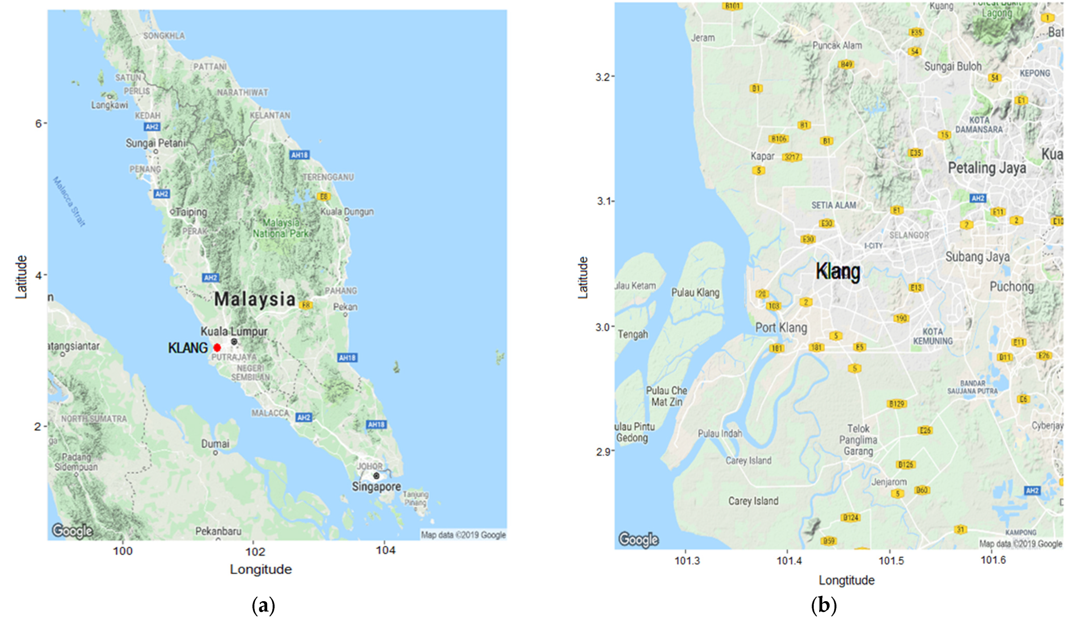
2. Study Area and Data

Klang is one of the largest cities in Malaysia, with a land area of approximately 573 km2. It is located at a latitude of 101°26′44.02″ E and longitude of 3°2′41.70″ N. Figure 1 shows the map of Peninsular Malaysia with the Klang location [36]. Klang is actively involved with many important industrial and economic interests for Malaysia and is a center for import and export activities that operate in Port Klang. Klang has been recognized as the 13th busiest trans-shipment port and the 16th busiest container port in the world. However, this scenario has elevated the risk of atmospheric pollution in Klang. In conjunction with this issue, the API behavior in Klang must be analyzed to facilitate the planning and mitigation of the risks of extreme air pollution events. Thus, hourly API data for the period covering 1 January 1997 to 31 August 2020 are analyzed in this study.
In Malaysia, air quality status at a particular time is measured using the Air Pollution Index (API). The API was first adopted and established in 1996 by the Department of Environment Malaysia to provide comprehensible information about the status of air quality to the public. The technique used to develop the API is almost similar with the Pollutant Standard Index by the United States Environmental Protection Agency [37,38]. Generally, information on five dominant sub-pollutant indices, namely, nitrogen dioxide (NO2), sulfur dioxide (SO2), ozone (O3), suspended particulate matter of less than 10 microns (PM10), and carbon monoxide (CO), are integrated, with the highest values of these indices representing the API values at a particular time. According to Al-Dhurafi et al. [39], PM10 and O3 are the main emission sources in this region.
Figure 2 illustrates the process of determining the API value. On the basis of the API value, the breakpoints of 50, 100, 200, 300, 400, and 500 are referred to as thresholds for categorizing API values that correspond to their associated health status [38,40], as described in Table 1.

3. Statistical Methodologies

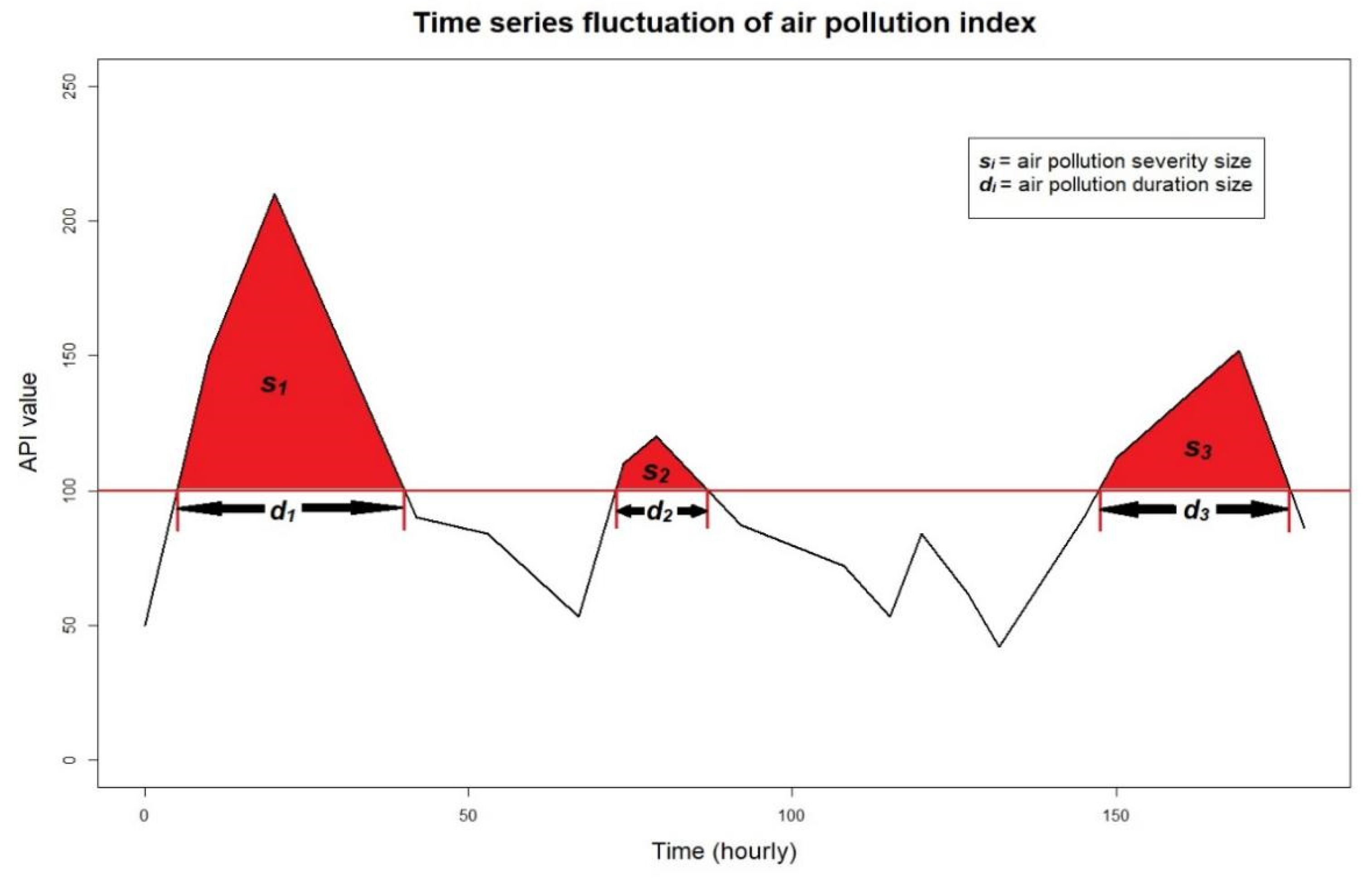
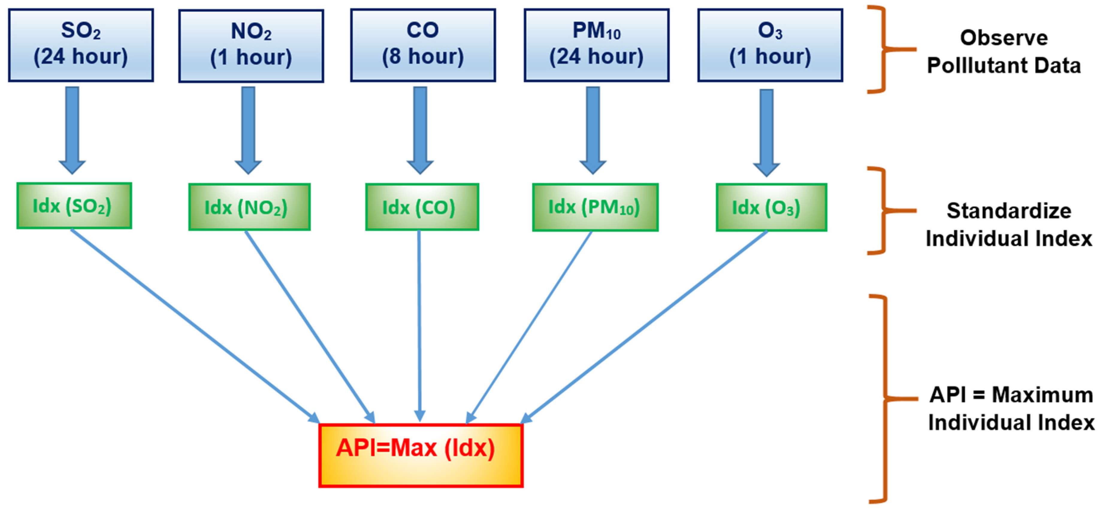
3.1. Air Pollution Severity Size

Based on Table 1, an API value higher than 100 indicates the occurrence of unhealthy air pollution events. Thus, information about the duration of unhealthy events can be derived based on consecutive API values higher than 100 that occur for a consistent period. Specifically, the duration of unhealthy air pollution events can be described mathematically as [42]:
D i = j = 1 N I i A P I j , f o r i = 1 , 2 , 3 , , n ,
where D i represents a random variable for pollution duration, j = 1, 2, 3, …, N represents an observe time series data with N is the total number of observations, and i = 1, 2, 3, …, n represents i-th air pollution event with n as the total number of air pollution events that occur throughout the period of 1 January 1997 to 31 August 2020. Then, for each particular i-th air pollution event, the indicator function I i A P I j is used to represent a data points with unhealthy state (API > 100) as follows:
I i A P I j = 1 , i f A P I j > 100 , 0 , i f A P I j 100 .
In addition, based on the duration size, this study proposes another characteristic of air pollution event, i.e., severity. Severity can be measured as cumulative API values greater than 100 that correspond to their duration D i . Mathematically, severity can be described as:
S i = j = 1 D i A P I j , f o r D i ,
where S i represents a random variable for the severity of pollution events. The higher the value of severity, the more serious the air pollution event [41]. The relationship between these two air pollution characteristics is illustrated in Figure 3. A prolonged duration of any unhealthy pollution event implies a high level of severity of that particular event, which indicates the occurrences of extreme pollution event. This scenario negatively affects public health, disrupts economic activities, and deteriorates environmental ecosystems. Thus, this study proposes the application of the extreme-value approach as a tool to evaluate the behavior of pollution severity and thus provide an improved understanding regarding this matter.

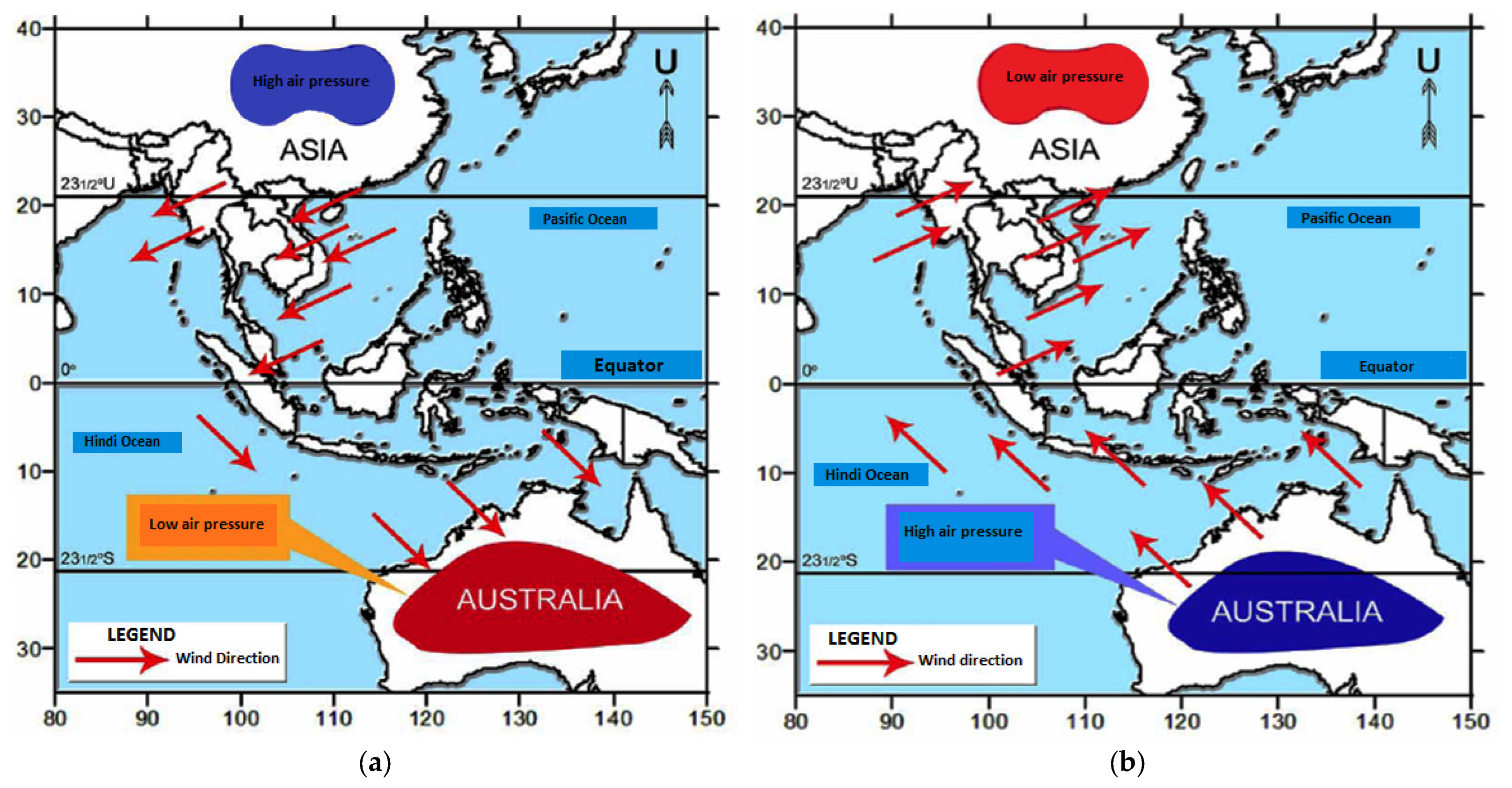
3.2. Maximum-Values Based on Monsoon Seasons

The pollution concentration in Klang is positively correlated with ambient temperature but negatively correlated with humidity factor. This scenario has been reported by Azmi et al. [43], who found that a high temperature increases the quantity of biomass burning and the re-suspension of materials, such as soil dust from the Earth’s surface. By contrast, high humidity influences the number of rain events, where the number of particles is reduced due to the wash-out processes of the atmospheric aerosols in the atmosphere. In addition, wind speed and UV radiation variables were found to have an effect on the concentration of particulate matter in the Klang area. All these factors can be related to the occurrence of monsoon seasons in Malaysia. Thus, this study investigates extreme pollution behavior by integrating information on monsoon seasons, which is used as block maxima on the generalized extreme-value (GEV) model.
Malaysia experiences recurrent annual monsoon seasons known as northeast and southwest monsoons. The northeast monsoon commonly occurs from November to March. This monsoon occurs in tandem with the winter season on the Asian continent. At the same time, the summer season occurs on the Australian continent. Thus, the Asian continent experiences low temperature (high-pressure area) while the Australian continent is having high temperature (low-pressure area). This phenomenon leads to the movement of wind from the high-pressure area of Asia to the low-pressure area of Australia due to the difference of temperature between these two continents. At this time, the wind blows at a speed of 10–20 knots, with its direction coming from the east or northeast of Peninsular Malaysia and then deflected toward Australia when crossing the Equator. By contrast, the southwest monsoon commonly occurs from June to September. During this period, the process is reversed, i.e., the Asian continent is having the summer season while the Australian continent is having the winter season. Thus, the winds blow from the Australian continent (with low air temperature and high pressure) to the Asian continent (with high air temperature and low pressure). The wind at this period blows with a speed of 15 knots, with its direction coming from Australia to the northwest across the Indian Ocean, and while crossing the Equator, the wind is deflected to the northeast before arriving southwest of Peninsular Malaysia. Both of these monsoon seasons bring heavy rains, which imply a decrease in temperature and increase in humidity [44]. Figure 4 illustrates the process of the northeast and southwest monsoon seasons in Malaysia. In between these two monsoon seasons, transition monsoon seasons commonly occur in April–May and September–October. During these periods, the wind blows at a lower speed (less than 10 knots) and fluctuates in terms of its direction. Moreover, humidity decreases and temperature increases during the period.
To summarize, each different monsoon season exhibits different meteorological phenomena that influence the behaviors of air pollution events. Thus, a maximum value of API data between different monsoon seasons will intrinsically provide good independent properties of extreme events. In this study, for the purpose of extreme-value modeling and analysis, a block maxima size will be determined based on four different monsoon seasons.

3.3. Extreme-Value Modeling

The block-maxima approach provides a tool to determine an extreme air pollution event that can be described by using an extreme-value model [45,46]. Let random variable X 1 , X 2 , , X n indicate severity data, which intrinsically follow a density function F. Then, to evaluate an extreme event, the maximum value of severity on some blocks Y = max X 1 , X 2 , , X n need to be determined. In parallel, the probability behavior of the extreme event dictated by the density function of the random variable Y can be determined as follows:
P Y y = P X 1 x , X 2 x , , X n y = F n y .
Although the independent and identical conditions on original random variable X 1 , X 2 , , X n are not satisfied, the density of F n may still be able to provide an accurate approximation probability model for the distribution of Y [47]. This flexibility enables an extreme-value model based on the block-maxima approach to be a popular tool for analyzing various kinds of problems, including a complex phenomenon [48,49,50]. However, in real applications, an exact density function of F that represents the distribution of the phenomenon being studied is always unknown. Thus, before implementing it in Equation (4), F is estimated on the basis of the observed data. However, small discrepancies in terms of F determination lead to substantial discrepancies of F n . This scenario affects the subsequent analysis involving F n , thus contributing to a large error that consequently produces wrong results. Fortunately, this problem can be overcome by assuming the density function F to be unknown. Then, F n can be obtained as an approximation to the limiting form of its density function [51]. This limiting distribution G y is valid if a sequence of constants a n > 0 and c n exists such that:
P Y c n a n y G y , a s n ,
where G y is also a nondegenerate function [52]. As described in various literature, a statistical model that satisfies the limiting distribution properties in Equation (5) is known as a GEV distribution, which is given as:
G y = exp 1 κ y ξ α 1 κ , f o r κ 0 , exp exp y ξ α , f o r κ = 0 ,
where ξ , α and κ indicate location, scale, and shape, respectively. Then, by inverting G y , its quantile function can be obtained [53] as:
G 1 p , ξ , α , κ = ξ + α κ 1 ln p κ , f o r κ 0 , ξ α ln ln p , f o r κ = 0 .
The information provided by the quantile function is useful for determining the return period of an extreme event. Return period is a popular tool in measuring a risk of recurrence of some extreme event [54,55]. Specifically, it measures the probability of the T-time block extreme event which exceeded is 1 T in every period of time which defined by block-maxima size. For a given return period x T , the critical value of the pollution severity can be determined on the basis of the following equation:
P Y > y T = G y T = 1 T .
Then, based on Equation (8), the estimated maximum pollution severity value corresponds to a particular return period, and T can be determined as:
y T = G 1 T 1 T , ξ , α , κ .

3.4. Methods of Parameter Estimation

The parameters of the GEV model need to be estimated in the process of modeling an extreme air pollution event. Three popular methods are considered in this study to determine the best fitted results in terms of the statistical modeling on severity size of air pollution event.

3.4.1. L-Moment Estimation

The L-moment method estimates the parameter of a model based on the concept probability weighted moment [56]. The L-moment estimators for the GEV model are given as follows:
ξ ^ = λ ^ 1 α ^ κ ^ 1 Γ 1 + κ ^ ,
α ^ = λ ^ 2 κ ^ 1 2 κ ^ Γ 1 + κ ^ ,
κ ^ = 7.859 c + 2.9554 c 2 ,
where c = 2 3 + τ ^ 3 log 2 log 3 . On the basis of Equations (10)–(12), the L-moment estimator for the terms of λ ^ 1 , λ ^ 2 , λ ^ 3 and τ ^ 3 = λ ^ 3 / λ ^ 2 must be estimated from the probability weighted moments determined from the following equation:
β r = ξ + α 1 r + 1 κ Γ 1 + κ κ r + 1 ,
such that, λ 1 = β 0 , λ 2 = 2 β 1 β 0 and λ 3 = 6 β 2 6 β 1 + β 0 [57]. Here, the unbiased estimator for β r is determined as follows [58]:
b r = i = 1 n i 1 i 2 i 3 i r n n 1 n 1 n r y i , f o r = 0 , 1 , 2 , ,

3.4.2. Maximum Likelihood Estimation (MLE)

The MLE method determines the value of the parameters such that they maximize the likelihood that the phenomenon described by the model produces data that are observed. On the basis of the GEV model in Equation (6), their log-likelihood function when κ 0 is given as follows:
l θ | y = n log α + i = 1 n 1 κ 1 ln z i z i 1 κ ,
where θ = ξ , α , κ and z i = 1 κ / α y i ξ [59,60]. Equation (15) does not provide an analytical solution for each parameter ξ , α and κ . Thus, a numerical optimization technique must be used to determine the final solution [52,61].

3.4.3. Generalized Maximum Likelihood Estimation (GMLE)

In the GMLE approach, the parameter κ in the GEV model is assumed to be a random variable with a range κ L , κ U and can be described by some form of beta prior density [60], given as:
π κ = 0.5 + κ p 1 0.5 + κ q 1 B p , q ,
where B p , q = Γ p Γ q / Γ p + q . Thus, on the basis of this prior density, the generalized likelihood function can be computed as:
G L ξ , α , κ | x = L ξ , α , κ | x π κ .
Then, the GMLE estimator for the parameters ξ , α and κ can be obtained by maximizing the generalized log-likelihood function, which corresponds to the modes of posterior distribution of their parameter. In this study, R software (Vienna, Austria) corresponding to extRemes package [61,62] is used to conduct extreme value analysis.

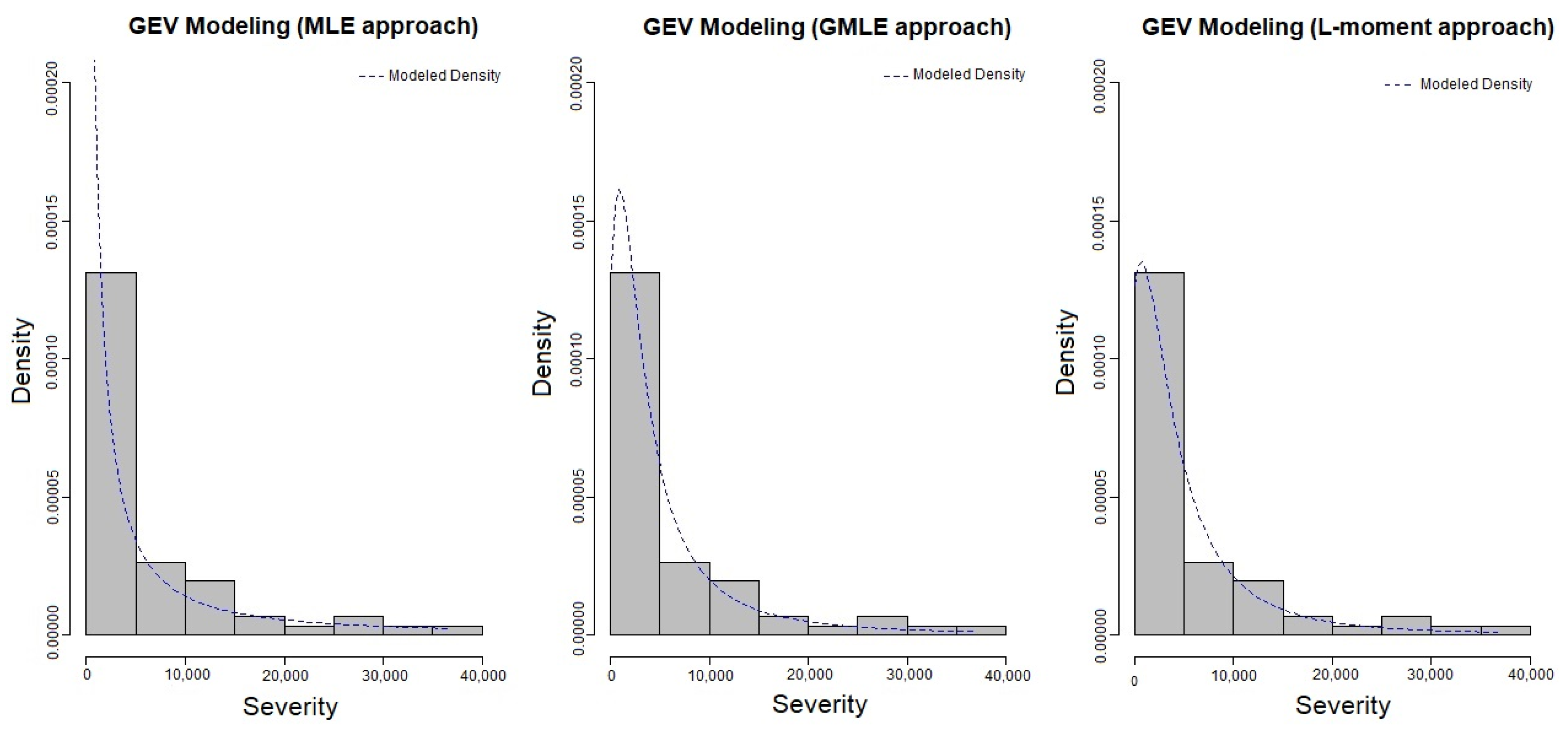
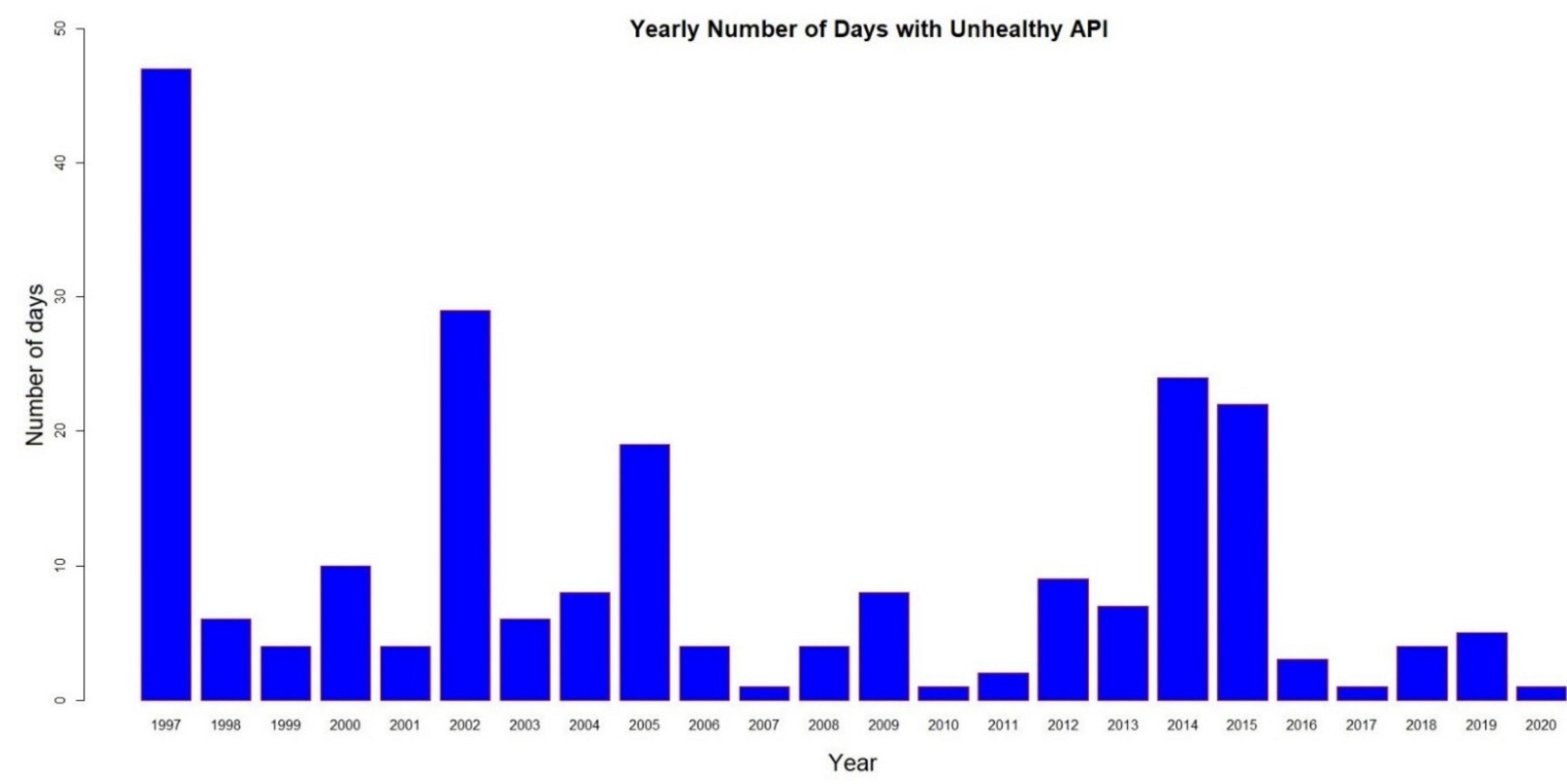
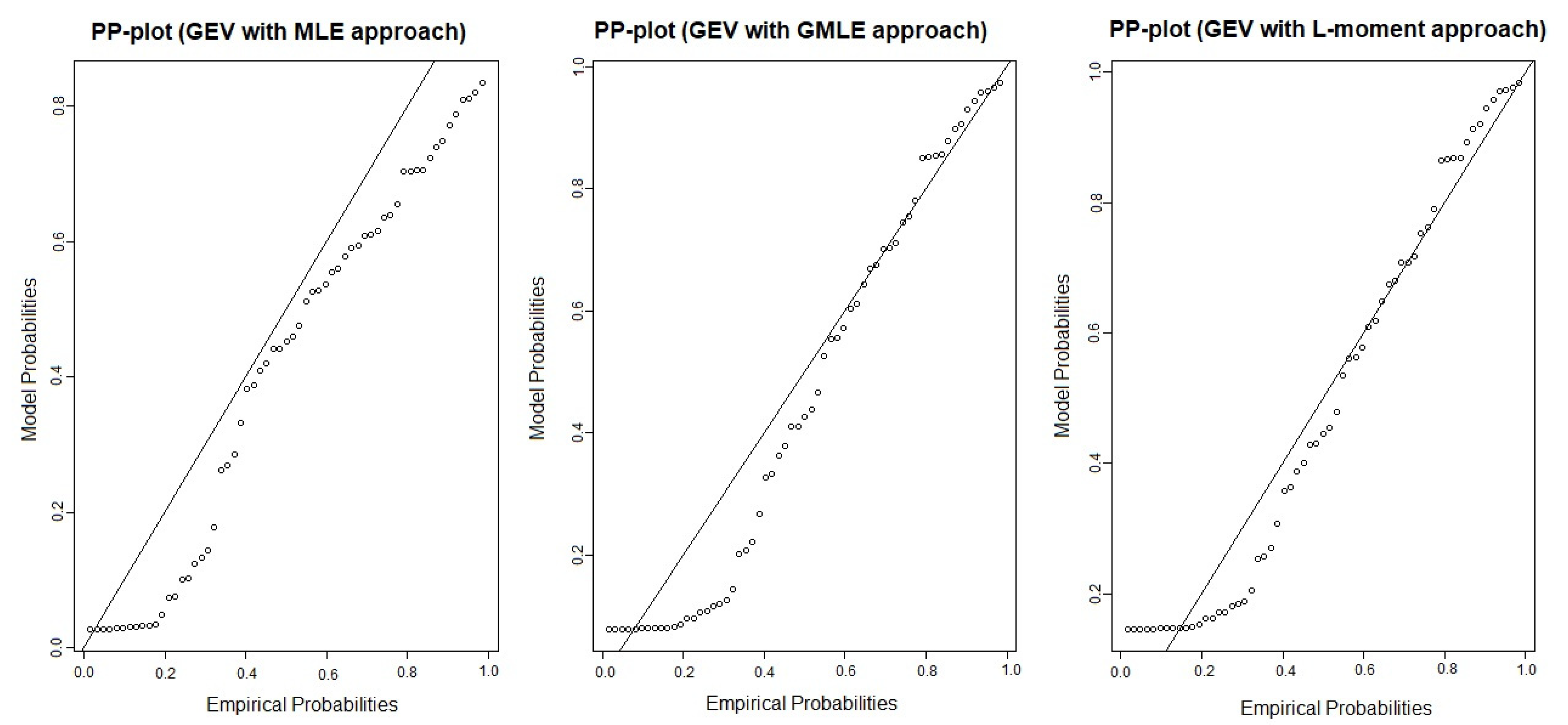
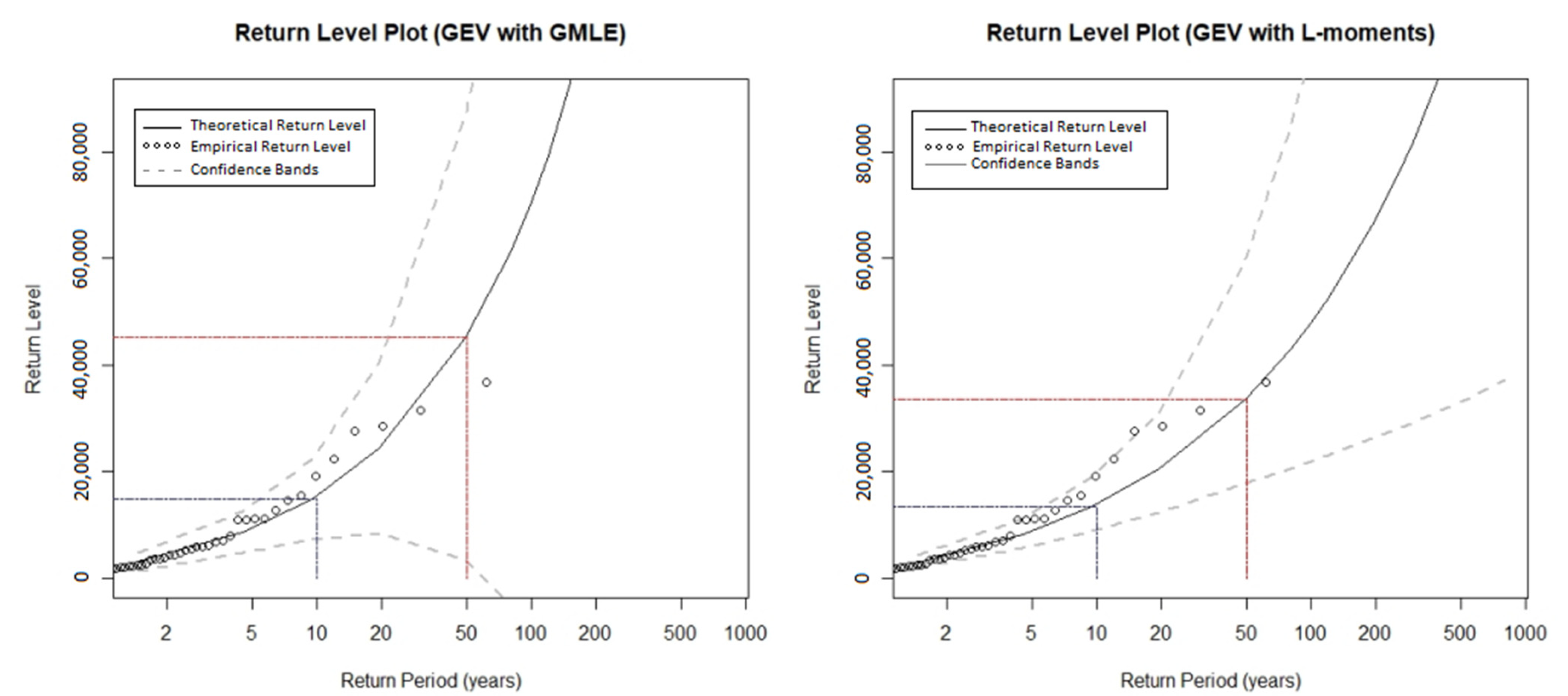
4. Results and Discussion

Before a detailed analysis is conducted, it is important to discuss some preliminary insights based on the descriptive statistics of the API data in Klang (presented in Table 2). Based on the observed hourly API data from January 1997 to August 2020, the mean API value is approximately 55.221 with a large standard deviation of 20.970, which indicates that the API value in Klang has high variability. The range of API values is also large, as determined by the difference between their minimum (0) and maximum (543) values. In addition, the measure of skewness and kurtosis indicates asymmetric behavior. These scenarios are presented clearly in Figure 5. The distribution of API data has a high variability accompanied with high skewness behavior due to long tail properties that exist in the upper tail of its distribution. Most of the time, the API status in Klang indicates a good (API < 50) and healthy (50 < API < 100) status. However, as mentioned previously, this study only investigates the occurrence of events above the unhealthy (API > 100) status, which could be defined as an unhealthy air pollution event. In particular, the proportion of data points (hourly) with unhealthy API is about 0.0245. That is, the total observed number of hours for unhealthy events (API > 100) from January 1997 to August 2020 is about 4980 h. In addition, Figure 6 shows the bar plot for yearly number of days with unhealthy API. Based on Figure 5 and Figure 6, the occurrences of extreme air pollution events represented by unhealthy, very unhealthy, hazardous, and emergency status is small. However, these events provide the most valuable information about the severity of a pollution event. These events exert negative effects on human health, disrupt economic activities, and deteriorate environmental ecosystems. Thus, these events are crucial for data analysis, particularly pollution risk management and mitigation.
Based on the API data, the severity size on each occurrence of an unhealthy air pollution event (API > 100) can be computed using their duration and severity measure as described in Equations (1) and (3). On a basis of severity data, a further investigation on the behavior of extreme pollution events can be done using a statistical analysis based on extreme-value model that corresponds to the maxima block approach on each monsoon season. Table 3 shows a comparison of the parameter estimations for the fitted GEV model. A different estimation method is found to produce a different result. Thus, the method that produces a more accurate result must be determined before a conclusion can be derived from the fitted GEV model. Based on the results of parameter estimation, Figure 7 and Figure 8 show a graphical representation of the model fitted. Both figures indicate that MLE is not a good method to deal with this issue. By contrast, the GMLE and L-moment methods produce good results with almost a similar performance. The fitted GEV density plots based on GMLE and L-moment are found to be able to represent well the extreme severity size of pollution event in Klang. The same conclusion can be drawn from a PP-plot, in which the model probabilities for each data point are found to indicate a smaller difference from their empirical probabilities. These findings are consistent with the results of the estimator analysis that have been reported by Martins and Stedinger [60].
Based on the fitted GEV model, information regarding the return period and return level of the severity size can be determined to measure the risk of recurrent extreme air pollution events. Return period provides information about the estimated time interval between the re-occurrence of some particular return level [63,64]. In this study, a return level refers to air pollution events with a particular level of severity size. For example, if a return period of some particular air pollution event is about 10 years, then its probability of occurring is equal to 1/10 during any one monsoon season. However, it does not mean that if an air pollution event has occurred within a 10-year return period, then the next air pollution event will occur within the next 10-year period as well. To the contrary, this means that, in any given monsoon season, there is a 10% chance that an air pollution event will occur, regardless of when the last similar event occurred. Figure 9 shows the results of return level estimates based on the GMLE and L-moment approaches. Both plots show that the estimated return level curves are found to be similar within the range of the observed data. However, for the range beyond the observed data, the interpolation of severity return level indicates differences. The return level estimate for maximum severity size based on GEV modeling with GMLE is found to be increased even more in comparison with the return level estimate based on GEV modeling with the L-moment approach. The confidence intervals of GEV modeling with GMLE are found to be much wider than GEV modeling with the L-moment approach, particularly for long return periods. Given that a small uncertainty is desirable, GEV modeling with the L-moment approach could be trusted, which implies that its inferences to the data of air pollution duration would be preferred.
Based on Figure 9, the return period shows the dependence between the return period that referred to time interval between the re-occurrence of some particular magnitude of return level that corresponds to a level of air pollution severity size. In general, from Figure 9, it is found that the lower return level appears more often that the higher return level. For the estimation return period of less than 10 years, both plots provide a good approximation. This result provides an agreement with Figure 7 and Figure 8, i.e., the GEV model is an appropriate approach to provide the estimation of the return level for extreme air pollution events, particularly for a period of less than 10 years. In parallel, Table 4 presents the results of the return level estimation of air pollution severity in a short return period of extreme pollution events.
According to Masseran [41], the air pollution events with a severity size greater than 1221 obey the power-law mechanism. The power-law mechanism describes the occurrence of extreme events corresponding to the existence of a long-tail properties (rare phenomena) in their distribution. Thus, it does not matter whether the pollution event is occurring with a duration of 10 days with 120 severity size, or in a single-day pollution incident with an API of 300. As long as the cumulative effect of API severity size for any pollution event is found to be greater than 1221, it is advisable that precautionary measures should be taken. Table 4 justifies that in the current scenarios, without any intervention, the estimated return levels for air pollution severity in Klang are found to exceed the threshold of 1221 within a period of 10 years. This scenario is most likely to occur in parallel with various related factors, particularly (i) rapid development around the Klang area involving the construction of many new houses and factories [65], and (ii) increasing in the number of motor vehicles [66]. This high severity implies a higher risk for the occurrences of pollution events that can negatively affect public health and disrupt the economic activities and environmental ecosystems of the country. Thus, additional prevention policies and stricter enforcement should be implemented to reduce and manage the risks of these extreme pollution events and thus improve environmental sustainability.

5. Conclusions

This study was conducted to deal with the issue of extreme air pollution events. For this purpose, an alternative measurement known as severity was proposed to represent the characteristic of extreme air pollution events. Specifically, information about severity is derived from the cumulative effect of air pollution events that can be determined from unhealthy API values that occur in a consecutive period. The higher the value of severity, the more serious is the air pollution event. On the basis of severity, an analysis of extreme air pollution events can be obtained through the application of the GEV model. A case study was conducted using hourly API data in Klang, Malaysia, from 1 January 1997 to 31 August 2020. Given that the air pollution in Malaysia is influenced by the effect of monsoon seasons, the block-maxima approach was integrated with information about monsoon seasons to determine suitable data points on GEV modeling. To determine the best-fitting GEV model, three different estimation methods were compared. The GMLE and L-moment methods can produce good GEV fitted results on modeling the severity size of air pollution events. On the basis of the fitted GEV model, information about the return period of extreme pollution severity in Klang was computed. The result showed a high expected level of severity size for unhealthy air pollution events in Klang. This result implies a higher risk of occurrences of pollution events with a high severity size that can negatively affect public health and disrupt the economic activities and environmental ecosystems of the country. Thus, additional prevention policies and stricter enforcement must be implemented to reduce and manage the risk of these extreme pollution events and thus improve environmental sustainability. However, a limitation of this study is related to interpolation of air pollution severity size for a long return period, in which the confidence interval for interpolation is found to be wider and corresponds to a longer duration of return periods. This scenario implies a decreasing precision of interpolation. Thus, for future research this study recommends the adaption of Bayesian technique with a proper prior knowledge on the parameters of GEV model to be overcome this issue.

Author Contributions

Conceptualization, methodology, formal analysis, visualization, writing—original draft preparation, funding acquisition, N.M.; validation, writing—review and editing M.A.M.S. All authors have read and agreed to the published version of the manuscript.

Funding

This research was funded by Universiti Kebangsaan Malaysia, grant number GP-2021-K020446 and the APC was funded by Universiti Kebangsaan Malaysia, grant number PP-FST-2022.

Institutional Review Board Statement

Not applicable.

Informed Consent Statement

Not applicable.

Data Availability Statement

Due to confidentiality agreements, supporting data can only be made available to bona fide researchers subject to a non-disclosure agreement. Details of the data and how to request access are available from https://www.doe.gov.my/portalv1/en/ (accessed on 12 March 2020) at Department of Environment Malaysia.

Acknowledgments

The authors are indebted to the Malaysian Department of Environment for providing air pollution data.

Conflicts of Interest

The authors declare no conflict of interest.

References

  1. Thunis, P. On the validity of the incremental approach to estimate the impact of cities on air quality. Atmos. Environ. 2018, 173, 210–222. [Google Scholar]
  2. Yang, J.; Shi, B.; Shi, Y.; Marvin, S.; Zheng, Y.; Xia, G. Air pollution dispersal in high density urban areas: Research on the triadic relation of wind, air pollution, and urban form. Sustain. Cities Soc. 2020, 54, 101941. [Google Scholar]
  3. An, Z.; Jin, Y.; Li, J.; Li, W.; Wu, W. Impact of particulate air pollution on cardiovascular health. Curr. Allergy Asthma Rep. 2018, 18, 15. [Google Scholar]
  4. Sah, D.; Verma, P.K.; Kandikonda, M.K.; Lakhani, A. Pollution characteristics, human health risk through multiple exposure pathways, and source apportionment of heavy metals in PM10 at Indo-Gangetic site. Urban Clim. 2019, 27, 149–162. [Google Scholar]
  5. Whyand, T.; Hurst, J.R.; Beckles, M.; Caplin, M.E. Pollution and respiratory disease: Can diet or supplements help? A review. Respir. Res. 2018, 19, 79. [Google Scholar] [PubMed] [Green Version]
  6. Saud, B.; Paudel, G. The threat of ambient air pollution in Kathmandu, Nepal. J. Environ. Public Health 2018, 2018, 1504591. [Google Scholar]
  7. Mannucci, P.M.; Franchini, M. Health effects of ambient air pollution in developing countries. Int. J. Environ. Res. Public Health 2017, 14, 1048. [Google Scholar]
  8. Al-Kindi, S.G.; Brook, R.D.; Biswal, S.; Rajagopalan, S. Environmental determinants of cardiovascular disease: Lessons learned from air pollution. Nat. Rev. Cardiol. 2020, 17, 656–672. [Google Scholar]
  9. Elleuch, B.; Bouhamed, F.; Elloussaief, M.; Jaghbir, M. Environmental sustainability and pollution prevention. Environ. Sci. Pollut. Res. 2018, 25, 18223–18225. [Google Scholar]
  10. Ionescu, L. Leveraging green finance for low-carbon energy, sustainable economic development, and climate change mitigation during the COVID-19 pandemic. Rev. Contemp. Philos. 2021, 20, 175–186. [Google Scholar]
  11. Ionescu, L. Transitioning to a low-carbon economy: Green financial behavior, climate change mitigation, and environmental energy sustainability. Geopolit. Hist. Int. Relat. 2021, 13, 86–96. [Google Scholar]
  12. Hamanaka, R.B.; Mutlu, G.M. Particulate matter air pollution: Effects on the cardiovascular system. Front. Endocrinol. 2018, 9, 680. [Google Scholar] [CrossRef] [PubMed] [Green Version]
  13. Sanyal, S.; Rochereau, T.; Maesano, C.N.; Com-Ruelle, L.; Annesi-Maesano, I. Long-term effect of outdoor air pollution on mortality and morbidity: A 12-year follow-up study for Metropolitan France. Int. J. Environ. Res. Public Health 2018, 15, 2487. [Google Scholar] [CrossRef] [PubMed] [Green Version]
  14. Davidson, N.; Mariev, O.; Turkanova, S. Does income inequality matter for CO2 emissions in Russian regions? Equilibrium. Q. J. Econ. Econ. Policy 2021, 16, 533–551. [Google Scholar]
  15. Ionescu, L. Corporate environmental performance, climate change mitigation, and green innovation behavior in sustainable finance. Econ. Manag. Financ. Mark. 2021, 16, 94–106. [Google Scholar]
  16. Lu, J.G. Air pollution: A systematic review of its psychological, economic, and social effects. Curr. Opin. Psychol. 2020, 32, 52–65. [Google Scholar] [CrossRef]
  17. Lü, J.; Liang, L.; Feng, Y.; Li, R.; Liu, Y. Air pollution exposure and physical activity in China: Current knowledge, public health implications, and future research needs. Int. J. Environ. Res. Public Health 2015, 12, 14887–14897. [Google Scholar] [CrossRef] [PubMed]
  18. Vert, C.; Sánchez-Benavides, G.; Martínez, D.; Gotsens, X.; Gramunt, N.; Cirach, M.; Molinuevo, J.L.; Sunye, J.; Nieuwenhuijsen, M.J.; Crous-Bou, M.; et al. Effect of long-term exposure to air pollution on anxiety and depression in adults: A cross-sectional study. Int. J. Hyg. Environ. Health 2017, 220, 1074–1080. [Google Scholar] [CrossRef]
  19. Zhang, H.; Chen, J.; Wang, Z. Spatial heterogeneity in spillover effect of air pollution on housing prices: Evidence from China. Cities 2021, 113, 103145. [Google Scholar] [CrossRef]
  20. Cabaneros, S.M.; Calautit, J.K.; Hughes, B.R. A review of artificial neural network models for ambient air pollution prediction. Environ. Model. Softw. 2019, 119, 285–304. [Google Scholar] [CrossRef]
  21. Liu, D.-R.; Hsu, Y.-K.; Chen, H.-Y.; Jau, H.-J. Air pollution prediction based on factory-aware attentional LSTM neural network. Computing 2021, 103, 75–98. [Google Scholar]
  22. Mao, W.; Wang, W.; Jiao, L.; Zhao, S.; Liu, A. Modeling air quality prediction using a deep learning approach: Method optimization and evaluation. Sustain. Cities Soc. 2021, 65, 102567. [Google Scholar]
  23. Fan, H.; Zhao, C.; Yang, Y. A comprehensive analysis of the spatio-temporal variation of urban air pollution in China during 2014–2018. Atmos. Environ. 2020, 220, 117066. [Google Scholar]
  24. Liu, X.; Hadiatullah, H.; Tai, P.; Xu, Y.; Zhang, X.; Schnelle-Kreis, J.; Schloter-Hai, B.; Zimmermann, R. Air pollution in Germany: Spatio-temporal variations and their driving factors based on continuous data from 2008 to 2018. Environ. Pollut. 2021, 276, 116732. [Google Scholar] [PubMed]
  25. Kamińska, J.A. The use of random forests in modelling short-term air pollution effects based on traffic and meteorological conditions: A case study in Wrocław. J. Environ. Manag. 2018, 217, 164–174. [Google Scholar]
  26. Yu, M.; Cai, X.; Xu, C.; Song, Y. A climatological study of air pollution potential in China. Theor. Appl. Climatol. 2019, 136, 627–638. [Google Scholar]
  27. Hodgson, E.C.; Phillips, I.D. Seasonal variations in the synoptic climatology of air pollution in Birmingham, UK. Theor. Appl. Climatol. 2021, 146, 1421–1439. [Google Scholar]
  28. Bose, M.; Larson, T.; Szpiro, A.A. Adaptive predictive principal components for modeling multivariate air pollution. Environmetrics 2018, 29, e2525. [Google Scholar]
  29. Hajmohammadi, H.; Heydecker, B. Multivariate time series modelling for urban air quality. Urban Clim. 2021, 37, 100834. [Google Scholar]
  30. Masseran, N.; Hussain, S.I. Copula modelling on the dynamic dependence structure of multiple air pollutant variables. Mathematics 2020, 8, 1910. [Google Scholar]
  31. Todorov, V.; Dimov, I. Innovative digital stochastic methods for multidimensional sensitivity analysis in air pollution modelling. Mathematics 2022, 10, 2146. [Google Scholar]
  32. Masseran, N. Modeling the characteristics of unhealthy air pollution events: A copula approach. Int. J. Environ. Res. Public Health 2021, 18, 8751. [Google Scholar] [PubMed]
  33. Vivanco-Hidalgo, R.M.; Avellaneda-Gómez, C.; Dadvand, P.; Cirach, M.; Ois, Á.; González, A.G.; Rodriguez-Campello, A.; de Ceballos, P.; Basagaña, X.; Zabalza, A.; et al. Association of residential air pollution, noise, and greenspace with initial ischemic stroke severity. Environ. Res. 2019, 179, 108725. [Google Scholar]
  34. Domingo, J.L.; Rovira, J. Effects of air pollutants on the transmission and severity of respiratory viral infections. Environ. Res. 2020, 187, 109650. [Google Scholar] [PubMed]
  35. Marquès, M.; Domingo, J.L. Positive association between outdoor air pollution and the incidence and severity of COVID-19. A review of the recent scientific evidences. Environ. Res. 2022, 203, 111930. [Google Scholar]
  36. Google Maps. 2019. Available online: https://www.google.com/maps/place/Klang,+Selangor/@3.2467558,101.2650693,9.1z/data=!4m5!3m4!1s0x31cc534c4ffe81cf:0xeb61f5772fd54514!8m2!3d3.044917!4d101.4455621 (accessed on 23 March 2019).
  37. Dominick, D.; Juahir, H.; Latif, M.T.; Zain, S.M.; Aris, A.Z. Spatial assessment of air quality patterns in Malaysia using multivariate analysis. Atmos. Environ. 2012, 60, 172–181. [Google Scholar]
  38. Department of Environment. A Guide to Air Pollutant Index in Malaysia (API); Ministry of Science, Technology and the Environment: Kuala Lumpur, Malaysia, 1997; Available online: https://aqicn.org/images/aqi-scales/malaysia-api-guide.pdf (accessed on 5 June 2018).
  39. Al-Dhurafi, N.A.; Masseran, N.; Zamzuri, Z.H.; Razali, A.M. Modeling unhealthy air pollution index using a peaks-over-threshold method. Environ. Eng. Sci. 2018, 35, 101–110. [Google Scholar]
  40. Masseran, N.; Razali, A.M.; Ibrahim, K.; Latif, M.T. Modeling air quality in main cities of Peninsular Malaysia by using a generalized Pareto model. Environ. Monit. Assess. 2016, 188, 65. [Google Scholar]
  41. Masseran, N. Power-law behaviors of the severity levels of unhealthy air pollution events. Nat. Hazards 2022, 112, 1749–1766. [Google Scholar]
  42. Masseran, N. Power-law behaviors of the duration size of unhealthy air pollution events. Stoch. Environ. Res. Risk Assess. 2021, 35, 1499–1508. [Google Scholar]
  43. Azmi, S.Z.; Latif, M.T.; Ismail, A.S.; Juneng, L.; Jemain, A.A. Trend and status of air quality at three different monitoring stations in the Klang Valley, Malaysia. Air Qual. Atmos. Health 2010, 3, 53–64. [Google Scholar] [PubMed] [Green Version]
  44. Ku Yaacob, K.K.; Ali, A.; Mohd Isa, M. Keadaan Laut Perairan Semenanjung Malaysia Untuk Panduan Nelayan. Jabatan Perikanan Malaysia. 2007. Available online: https://repository.seafdec.org.my/bitstream/handle/20.500.12561/313/Keadaan%20Laut%20Perairan%20Semenanjung%20Malaysia%20Untuk%20Panduan%20Nelayan_DPPSPM%20DOF.pdf?sequence=1&isAllowed=y (accessed on 25 February 2019).
  45. Kütchenhoff, H.; Thamerus, M. Extreme value analysis of Munich air pollution data. Environ. Ecol. Stat. 1996, 3, 127–141. [Google Scholar]
  46. Reyes, H.J.; Vaquera, H.; Villaseñor, J.A. Estimation of trends in high urban ozone levels using the quantiles of (GEV). Environmetrics 2010, 21, 127–141. [Google Scholar]
  47. Reiss, R.-D.; Thomas, M. Statistical Analysis of Extreme Values: With Application to Insurance, Finance, Hydrology and Other Fields; Die Deutsche Bibliothek: Berlin, Germany, 2007. [Google Scholar]
  48. French, J.; Kokoszka, P.; Stoev, S.; Hall, L. Quantifying the risk of heat waves using extreme value theory and spatio-temporal functional data. Comput. Stat. Data Anal. 2019, 131, 176–193. [Google Scholar]
  49. Panagoulia, D.; Economou, P.; Caroni, C. Stationary and nonstationary generalized extreme value modelling of extreme precipitation over a mountainous area under climate change. Environmetrics 2014, 25, 29–43. [Google Scholar]
  50. Yoon, S.; Kumphon, B.; Park, J.-S. Spatial modeling of extreme rainfall in northeast Thailand. J. Appl. Stat. 2015, 42, 1813–1828. [Google Scholar]
  51. Cocchi, D.; Scagliarini, M. Modelling extreme rainfall data within a catchment region. Environmetrics 2003, 14, 11–26. [Google Scholar]
  52. Coles, S. An Introduction to Statistical Modeling of Extreme Values; Springer: London, UK, 2001. [Google Scholar]
  53. Scotto, M.G.; Barbosa, S.M.; Alonso, A.M. Extreme value and cluster analysis of European daily temperature series. J. Appl. Stat. 2011, 38, 2793–2804. [Google Scholar]
  54. Katz, R.W.; Parlange, M.B.; Naveau, P. Statistics of extremes in hydrology. Adv. Water Resour. 2002, 25, 1287–1304. [Google Scholar]
  55. Sadegh, M.; Moftakhari, H.; Gupta, H.V.; Ragno, E.; Mazdiyasni, O.; Sanders, B.; Matthew, R.; AghaKouchak, A. Multihazard scenarios for analysis of compound extreme events. Geophys. Res. Lett. 2018, 45, 5470–5480. [Google Scholar]
  56. Hosking, J.R.M. L-Moments: Analysis and estimation of distributions using linear combinations of order statistics. J. R. Stat. Soc. Ser. B Stat. Methodol. 1990, 52, 105–124. [Google Scholar] [CrossRef]
  57. Lee, S.H.; Maeng, S.J. Frequency analysis of extreme rainfall using L-moment. Irrig. Drain. 2003, 52, 219–230. [Google Scholar] [CrossRef]
  58. Noto, L.V.; La Loggia, G. Use of L-moments approach for regional flood frequency analysis in Sicily, Italy. Water Resour. Manag. 2009, 23, 2207–2229. [Google Scholar] [CrossRef]
  59. Hosking, J.R.M. Algorithm as 215: Maximum-likelihood estimation of the parameters of the generalized extreme-value distribution. J. R. Stat. Soc. Ser. C Appl. Stat. 1985, 34, 301–310. [Google Scholar] [CrossRef]
  60. Martins, E.S.; Stedinger, J.R. Generalized maximum-likelihood generalized extreme-value quantile estimators for hydrologic data. Water Resour. Res. 2000, 36, 737–744. [Google Scholar] [CrossRef]
  61. Gilleland, E.; Katz, R.W. extRemes 2.0: An extreme value analysis package in R. J. Stat. Softw. 2016, 72, 1–39. [Google Scholar] [CrossRef] [Green Version]
  62. Gilleland, E. extRemes: Extreme Value Analysis. R Package Version 2.1-2. Available online: https://cran.r-project.org/web/packages/extRemes/extRemes.pdf (accessed on 4 June 2021).
  63. Cooley, D. Return periods and return levels under climate change. In Extremes in a Changing Climate. Water Science and Technology Library; AghaKouchak, A., Easterling, D., Hsu, K., Schubert, S., Sorooshian, S., Eds.; Springer: Dordrecht, The Netherlands, 2013; Volume 65, pp. 97–114. [Google Scholar]
  64. McPhillips, L.E.; Chang, H.; Chester, M.V.; Depietri, Y.; Friedman, E.; Grimm, N.B.; Kominoski, J.S.; McPhearson, T.; Méndez-Lázaro, P.; Rosi, E.J.; et al. Defining extreme events: A cross-disciplinary review. Earth’s Future 2018, 6, 441–455. [Google Scholar] [CrossRef]
  65. Usmani, R.S.A.; Saeed, A.; Abdullahi, A.M.; Pillai, T.R.; Jhanjhi, N.Z.; Hashem, I.A.T. Air pollution and its health impacts in Malaysia: A review. Air Qual. Atmos. Health 2020, 13, 1093–1118. [Google Scholar] [CrossRef]
  66. Chin, Y.S.J.; De Pretto, L.; Thuppil, V.; Ashfold, M.J. Public awareness and support for environmental protection–A focus on air pollution in peninsular Malaysia. PLoS ONE 2019, 14, e0212206. [Google Scholar]
Figure 1. (a) Map of Peninsular Malaysia. Klang is identified by the red dot; (b) Map of Klang.
Mathematics 10 03004 g001
Figure 2. Process of determining the API value [41].
Mathematics 10 03004 g002
Figure 3. Air pollution characteristics based on their duration and severity [32].
Mathematics 10 03004 g003
Figure 4. Process of the formation of the (a) northeast and (b) southwest monsoon seasons in Malaysia [44].
Mathematics 10 03004 g004
Figure 5. Distribution of API data in Klang corresponds to their air quality status.
Mathematics 10 03004 g005
Figure 6. Bar plot for yearly number of days with unhealthy API.
Mathematics 10 03004 g006
Figure 7. Comparison of GEV modeling using different estimation methods.
Mathematics 10 03004 g007
Figure 8. PP-plot on the fitted GEV model based on different estimation approaches.
Mathematics 10 03004 g008
Figure 9. Return level estimates based on the GMLE and L-moment approaches.
Mathematics 10 03004 g009
Table 1. API values and their corresponding health effects and advice.
APIStatusHealth EffectHealth Advice
0–50GoodLow pollution without a bad effect on health.Outdoor activities are not restricted.
Maintain healthy lifestyle.
51–100ModerateModerate pollution that does not pose any bad effect on health.Outdoor activities are not restricted.
Maintain healthy lifestyle.
101–200UnhealthyWorsens the health condition of high-risk people, i.e., people with heart and lung complications.Outdoor activities for high-risk people are limited. The public needs to reduce extreme outdoor activities.
201–300Very UnhealthyWorsens the health condition and lowers tolerance to physical exercises of people with heart and lung complications, affects public health.Elderly and high-risk people are prohibited from outdoor activities. The public is advised to refrain from outdoor activities.
301–500HazardousHazardous to high-risk people and public health.Elderly and high risk people are prohibited from outdoor activities. The public is advised to refrain from outdoor activities.
>500EmergencyHazardous to high-risk people and public health.The public is advised to follow orders from the National Security Council and always follow the announcements in mass media.
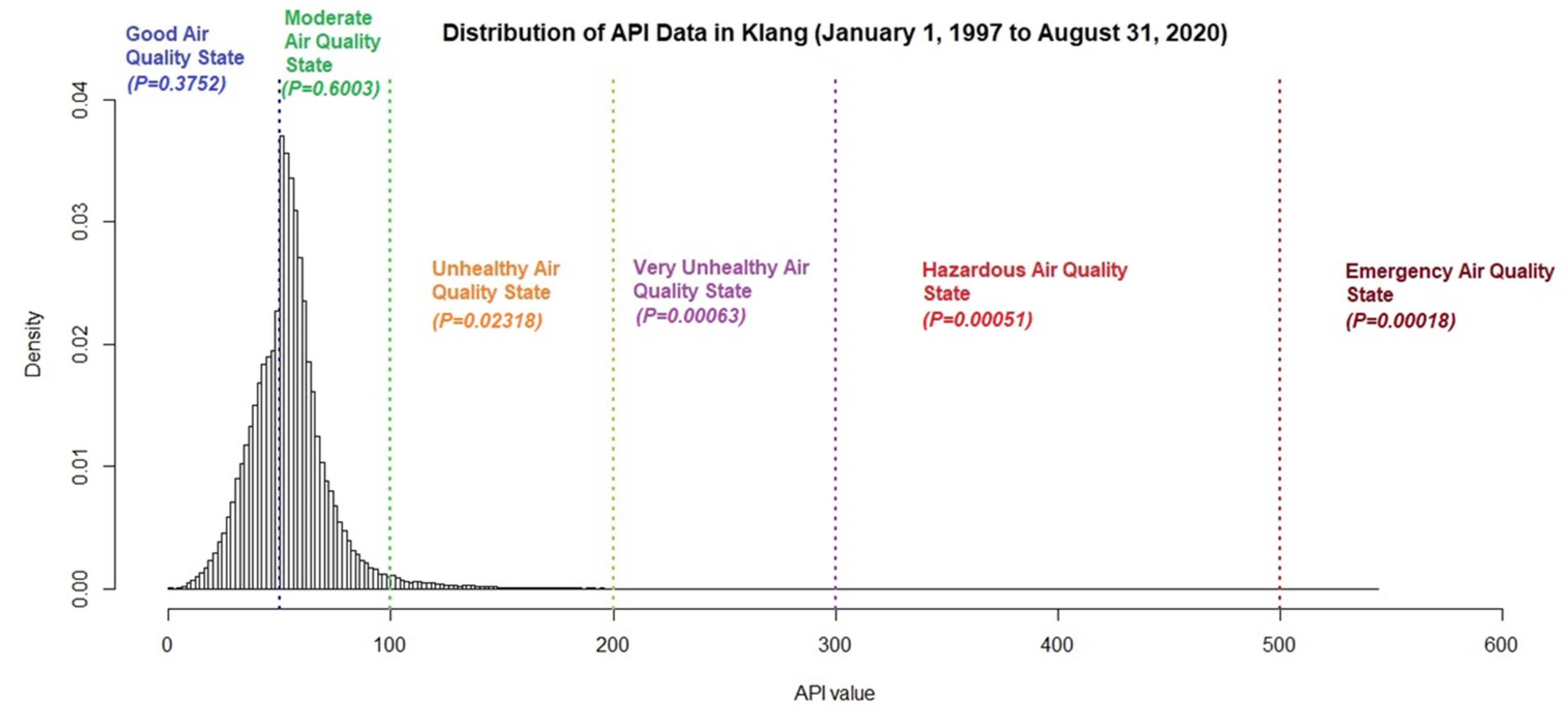
Table 2. Descriptive statistics for the air pollution data in Klang.
DataMeanMinimumMaximumStd. DeviationSkewnessKurtosis
Observed API55.221054320.9704.53765.133
Table 3. Comparison of the results of parameter estimation for the fitted GEV model.
ModelEstimated Parameter
Location   ( ξ ) Scale   ( α ) Shape   ( κ )
GEV based on L-moments1790.6612975.9360.452
GEV based on MLE1584.3592997.8201.824
GEV based on GMLE1996.1372663.2160.613
Table 4. Return level estimates corresponding to their return period.
Return PeriodReturn Level Estimation Air Pollution Severity
2 years3090.557
3 years5206.969
5 years6975.709
6 years8546.659
7 years11,319.008
8 years12,576.375
9 years13,769.592
10 years14,909.100
Publisher’s Note: MDPI stays neutral with regard to jurisdictional claims in published maps and institutional affiliations.

