Hybrid Nanofluid Radiative Mixed Convection Stagnation Point Flow Past a Vertical Flat Plate with Dufour and Soret Effects

Abstract

The widespread application of hybrid nanofluid in real applications has been accompanied by a large increase in computational and experimental research. Due to the unique characteristics of hybrid nanofluid, this study aspires to examine the steady two-dimensional mixed convection stagnation point flow of a hybrid nanofluid past a vertical plate with radiation, Dufour, and Soret effects, numerically. The formulations of the specific flow model are presented in this study. The model of fluid flow that is expressed in the form of partial differential equations is simplified into ordinary differential equations via the transformation of similarity, and then solved numerically by using the boundary value problem solver known as bvp4c in MATLAB, which implements the finite difference scheme with the Lobatto IIIa formula. Two possible numerical solutions can be executed, but only the first solution is stable and meaningful from a physical perspective when being evaluated via a stability analysis. According to the findings, it is sufficient to prevent the boundary layer separation by using 2% copper nanoparticles and considering the lesser amount of Dufour and Soret effects. The heat transfer rate was effectively upgraded by minimizing the volume fraction of copper and diminishing the Dufour effect. Stronger mixed convection would lead to maximum skin friction, mass transfer, and heat transfer rates. This important preliminary research will give engineers and scientists the insight to properly control the flow of fluids in optimizing the related complicated systems.

1. Introduction

Over the last few years, researchers and scientists have devoted a significant amount of attention to the progress made in creating sophisticated heat transfer fluids. In most industrial and technical applications, common fluids such as oil and water are employed. However, because of their poor thermal performance, the pace at which these fluids may transmit heat is restricted. As a result, to address this shortcoming, a singular type of nanosized particles has been integrated into the conventional fluid, and this fluid has been given the name “nanofluid”. In 1995, Choi [1] initially presented this fluid to the scientific community. According to various thorough reviews on nanofluid, researchers have consistently employed two nanofluid models: (i) Buongiorno [2] and (ii) Tiwari and Das [3], which have distinct mechanisms. To examine the behavior of nanofluids, Buongiorno creates a two-phase nanofluid model that considers thermophoresis and Brownian motion effects in the energy equation. Meanwhile, the nanofluid model established by Tiwari and Das is a one-phase model that specifically considers the thermophysical properties of the nanoparticles. Due to the necessity for theoretical and experimental knowledge, researchers have focused their efforts on this area in recent years. For example, Rizwana et al. [4] analyzed the unsteady oblique stagnation point flow of nanofluid with the implementation of Fourier Law to scrutinize the heat flux. Ferdows et al. [5] considered the boundary layer flow of various nanofluids such as silver–water, copper–water, alumina–water, and titania–water under the influence of a magnetic field in the non-isothermal and constant heat flux limits. The rate of entropy generation, heat, and solutal transfer of a nanofluid in an annular closure has been investigated in the presence of double-diffusive convection by Swamy et al. [6], and they observe that a shallow annulus may improve the thermal and solutal performance with minimum entropy production. Batool et al. [7] also considered the nanofluid in their investigation of fluid flow through the lid-driven cavity with the aim to improve the heat transfer process. Recently, Sankar et al. [8] explored the alumina–water nanofluid flow inside the vertical annular geometry with non-uniform heating. The augmentation of thermal transfer is facilitated through the addition of nanoparticles, but this also causes the flow strength to reduce [8]. However, despite the continuous investigations, the thermal performance of nanofluids is still limited and this then results towards the formation of hybrid nanofluid.

The discovery of hybrid nanofluid has contributed to the progress of nanotechnology and sparked researchers’ attention, motivating them to extend their experimental and numerical research. Suresh et al. [9] have experimentally explored the thermal performance of copper-alumina/water hybrid nanofluid. Their experiment noted that despite the poor thermal performance of alumina, its chemical inertness might help to preserve the stability of the fluid. Further, research on convective hybrid nanofluid flow in circular tubes was accomplished by Suresh et al. [10], at Re = 1730, the findings showed a 13.56% of increment in the Nusselt number. Moreover, in a review study conducted by Huminic and Huminic [11], it was also reported that hybrid nanofluid has great thermal performance and can improve the heat transfer in heat exchangers. This capability of hybrid nanofluid has been proven by experimental and computational studies [12,13]. Better heat transmission mechanisms are predicted to be developed using hybrid nanofluids, which are made up of a homogenous suspension of multiple nanoparticles attached by both chemical and physical bonds. Due to its usefulness in a variety of thermal applications (e.g., in pharmaceutical processes, fuel cells, and hybrid-powered engines), this novel kind of nanofluid’s primary goal is to improve the heat transmission, thermophysical, and hydrodynamic characteristics (see Shenoy et al. [14]). However, further research is needed to examine the alternative hybridizations of nanoparticles, their stability and mixing ratio, and the procedures that aid in the improvement of heat transfer. As a result of this, scientists are working incessantly to implement new hybrid nanofluids that have substantially greater thermal conductivities than typical viscous fluids (see Shenoy et al. [14] and Merkin et al. [15]). After browsing through the relevant literature, it is found that the hybrid nanofluid flow with various involvement of pertinent effects has been actively explored by several researchers, such as Abbas et al. [16,17] (for the hybrid nanofluid stagnation point flow with slip); Tulu and Ibrahim [18] (for the second-order velocity slip flow of hybrid nanofluid); Mahabaleshwar et al. [19] (for the stretching/shrinking flow); Khan et al. [20] (for the mixed convective flow); and Reddy et al. [21] (for the flow inside a heated annulus). In these mentioned studies, it seems that the nanofluid model by Tiwari and Das [3] has been mostly used in the formulations, while the hybrid nanofluid model that considers the Buongiorno [2] two-phase nanofluid model with the consideration of concentration equation is still limited in the literature.

An energy flux may be formed by concentration and temperature gradients when the mass and heat transfer happen concurrently. The Dufour (diffusion-thermo) effect refers to the energy flow that results from concentration gradients (see Rastogi and Madan [22]). Meanwhile, the Soret (thermal-diffusion) effect occurs due to the temperature gradients [23,24]. Due to their smaller-order magnitude, thermal-diffusion and diffusion-thermo processes are frequently overlooked in the heat transfer processes. However, as asserted by Seid et al. [25], these effects cannot be disregarded in flow systems that have large concentration and temperature gradients, which mostly occur in engineering processes such as in the process of chemical manufacture, material insulation, and foam combustion. Considering this fact, several researchers believed it would be beneficial to analyze the Dufour and Soret effects on a variety system of fluid flow. It is scrutinized by Salleh et al. [26] that in a specific range of velocity ratio, the heat transmission can be augmented when a stronger Soret effect is inserted, while concurrently lowering the Dufour effect. The impacts of Dufour and Soret towards the fluid flow past a vertical porous plate are investigated by Kumar et al. [27]. They report that the Soret effect increases the concentration profile but oppositely for the Dufour effect. The same conclusion has also been drawn by Jawad et al. [28] in their research on Darcy–Forchheimer radiative nanofluid flow with Marangoni convection. Meanwhile, in the study performed by Khan et al. [29] towards the non-Newtonian micropolar fluid flow of an expandable cylinder, the boost of the Dufour effect negatively impacted the temperature profile. Several other recent works of research regarding Dufour and Soret effects can be retrieved in the studies conducted by Salmi et al. [30], Yinusa et al. [31], Pal et al. [32], and Sheri et al. [33]. However, in most of these studies, the impact of Soret and Dufour effects towards the boundary layer flow separation is not reported and discussed.

Inspired by the previous studies while trying to bridge the research gap, the authors are inspired to examine the radiative mixed convection stagnation point flow of alumina-copper/water hybrid nanofluid past a vertical flat plate with Dufour and Soret effects, while extending the previous study reported by Srinivasacharya and RamReddy [34]. Several improvements and modifications that have been considered towards the model are listed as below:

• The model used by the previous study is modified towards the Tiwari and Das [3] nanofluid model.
• The fluid is upgraded to hybrid nanofluid by using the thermophysical correlations suggested by Takabi and Salehi [35] and the properties provided by Oztop and Abu-Nada [36].
• New additional effects such as the stagnation point flow, thermal radiation, and convective heated boundary condition are inserted towards the present model.
• The equations of the flow model are solved via a sophisticated solver known as bvp4c in MATLAB that could provide a better numerical solution.
• Two different alternative solutions are provided in the present study and the stability analysis has also been derived and reported to analyze the stability feature of the generated numerical solutions.
• The preferable value of parameters to control the skin friction, heat transfer, and mass transfer rates as well as the boundary layer separation process for the present model are highlighted and discussed in the findings.

Therefore, it is believed that this exploratory research is significant for the future benchmarking of real-world industrial processes and applications. Several applications of hybrid nanofluid that can be mentioned here are its use in heat exchangers and heat pipes; coolants in machining and manufacturing; generator cooling; refrigeration; solar collectors; and heating, ventilation, and air conditioning (HVAC) application [37]. It should also be noted here that the stagnation point flow is also important in many applications, for instance, in polymer extrusion, wire and plastic sheet drawing, nuclear reactor cooling, and other hydrodynamic applications [38]. Many industrial processes also consider the mixed convection flow, such as for the heating of material traveling between a feed roll and a wind-up roll or a conveyer belt, the extrusion of steel, the cooling of a large metallic plate in a bath, and liquid films in condensation processes [39]. Thus, the current results may give an insight, especially to the scientists working with nanofluids—specifically, those related to the flow with a mixed convection and stagnation point.

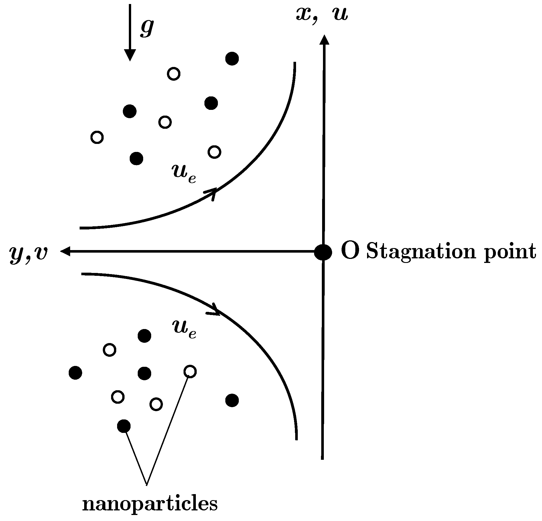
2. Mathematical Model

Generally, a vectorial version of a simple mathematical steady flow model of hybrid nanofluid may be written as [40,41]:

$$\nabla \cdot \overrightarrow{V}=0,$$

(1)

$${\rho }_{hnf}\left(\overrightarrow{V}\cdot \nabla \right)\overrightarrow{V}=-\nabla \overrightarrow{p}+{\mu }_{hnf}{\nabla }^2\overrightarrow{V},$$

(2)

$${\left(\rho C_p\right)}_{hnf}\left(\overrightarrow{V}\cdot \nabla \right)T=k_{hnf}{\nabla }^{2}T,$$

(3)

$$\left(\overrightarrow{V}\cdot \nabla \right)C=D_m{\nabla }^{2}C,$$

(4)

where $\overrightarrow{V}={\overrightarrow{u}}_i+{\overrightarrow{v}}_j$ is the velocity vector, ${\nabla }^2$ is the Laplacian operator, $\overrightarrow{p}$ is the total pressure force vector, $T$ is temperature, and $C$ is the solutal concentration for the hybrid nanofluid. Moreover, ${\mu }_{hnf}$ is the dynamic viscosity; ${\rho }_{hnf}$ is the density; $k_{hnf}$ is the thermal conductivity; ${(\rho C_p)}_{hnf}$ is the heat capacity; and ${(C_p)}_{hnf}$ is the specific heat capacity for the hybrid nanofluid.

In this study, the two-dimensional, steady, radiative, mixed convective, stagnation point flow of hybrid nanofluid (see Figure 1) is considered, where the Cartesian coordinates of the $x$-axis are assumed along the vertical plate and the $y$-axis is normal to it, with the flow being at $y\ge 0$. The velocity of the far (inviscid) flow is $u_e\left(x\right)=ax$ [42,43], where $a$ is a positive constant. It is assumed that the variable convective temperature $T_f\left(x\right)$ and variable concentration $C_w\left(x\right)$ at the plate are given as $T_f\left(x\right)=T_{\infty }+T_0\left(x/l\right)$ [44] and $C_w\left(x\right)=C_{\infty }+C_0\left(x/l\right)$ [45], where $T_0$ and $C_0$ are the characteristic temperature and concentration at the plate, $T_{\infty }$ and $C_{\infty }$ are the ambient temperature and concentration of the fluid, and $l$ is the characteristic length of the plate. Two distinct nanoparticles are considered in this study, namely, alumina and copper, diluted in the water base fluid. It is assumed that the nanoparticles have the same size and shape, and that the volume fraction considered would not result in collisional interactions. Presumably, the nanoparticles would not aggregate since they are uniformly dispersed and very small in size. Several pertinent effects such as mixed convection, convective boundary condition, thermal radiation, and Dufour and Soret effects are imposed towards the flow model.

Therefore, according to the assumptions, the appropriate equations for the present model can be constructed as follows [34,46]:

$$\frac{\partial u}{\partial x}+\frac{\partial v}{\partial y}=0,$$

(5)

$$u\frac{\partial u}{\partial x}+v\frac{\partial u}{\partial y}=u_e\frac{d{u}_e}{dx}+\frac{{\mu }_{hnf}}{{\rho }_{hnf}}\frac{{\partial }^{2}u}{\partial y^2}+{\beta }_{hnf}\left(T-T_{\infty }\right)g+{\beta }_c\left(C-C_{\infty }\right)g,$$

(6)

$$u\frac{\partial T}{\partial x}+v\frac{\partial T}{\partial y}=\frac{k_{hnf}}{{\left(\rho C_p\right)}_{hnf}}\frac{{\partial }^{2}T}{\partial y^2}-\frac{1}{{\left(\rho C_p\right)}_{hnf}}\frac{\partial q_r}{\partial y}+\frac{D_m}{C_s}\frac{k_T}{{\left(C_p\right)}_f}\frac{{\partial }^{2}C}{\partial y^2},$$

(7)

$$u\frac{\partial C}{\partial x}+v\frac{\partial C}{\partial y}=D_m\frac{{\partial }^{2}C}{\partial y^2}+\frac{D_m{k}_T}{T_m}\frac{{\partial }^{2}T}{\partial y^2},$$

(8)

subject to the boundary conditions

$$\left.\begin{array}{c}v=u=0,-k_{hnf}\frac{\partial T}{\partial y}=h_f\left(T_f-T\right),C\left(x\right)=C_w\left(x\right)\mathrm{at}y=0,\\ u\to u_e\left(x\right)=ax,T\to T_{\infty },C\to C_{\infty }\mathrm{as}y\to \infty ,\end{array}\right\}$$

(9)

where $u_e(d{u}_e/dx)$ denote the stagnation point term; ${\beta }_{hnf}(T-T_{\infty })g$ denote the mixed convection term; ${\beta }_c(C-C_{\infty })g$ denote the buoyancy ratio term; $-1/{(\rho C_p)}_{hnf}(\partial q_r/\partial y)$ denote the thermal radiation term; $(D_m{k}_T/C_s{(C_p)}_f)({\partial }^{2}C/\partial y^2)$ denote the Dufour effect term; and $(D_m{k}_T/T_m)({\partial }^{2}T/\partial y^2)$ denote the Soret effect term, in which $u$ and $v$ are the velocity along the $x$,$y$-axes; $C_s$ is the concentration susceptibility; ${\beta }_c$ is the solutal expansion coefficient; $k_T$ is the thermal diffusion ratio; $q_r$ is radiative heat flux; $g$ is the acceleration due to gravity; $T_m$ is the mean hybrid nanofluid temperature; $D_m$ is the solutal diffusivity of the medium; $h_f$ is the convective heat transfer coefficient; and ${\beta }_{hnf}$ is the thermal expansion for the hybrid nanofluid. The correlations relating to the thermophysical properties of hybrid nanofluid are presentable in

Table 1. Correlations for the thermophysical properties.

Properties	Hybrid Nanofluid
Density	${\rho }_{hnf}={\varphi }_{A{l}_2{O}_3}{\rho }_{A{l}_2{O}_3}+{\varphi }_{Cu}{\rho }_{Cu}+(1-{\varphi }_{hnf}){\rho }_f$ $\mathrm{where}{\varphi }_{hnf}={\varphi }_{A{l}_2{O}_3}+{\varphi }_{Cu}$
Heat capacity	${\left(\rho C_p\right)}_{hnf}={\varphi }_{A{l}_2{O}_3}{(\rho C_p)}_{A{l}_2{O}_3}+{\varphi }_{Cu}{(\rho C_p)}_{Cu}+\left(1-{\varphi }_{hnf}\right){(\rho C_p)}_f$
Dynamic viscosity	${\mu }_{hnf}={\mu }_f{\left(1-{\varphi }_{hnf}\right)}^{-2.5}$
Thermal conductivity	$\frac{k_{hnf}}{k_f}=\left[\frac{\left(\frac{{\varphi }_{A{l}_2{O}_3}{k}_{A{l}_2{O}_3}+{\varphi }_{Cu}{k}_{Cu}}{{\varphi }_{hnf}}\right)+2k_f+2\left({\varphi }_{A{l}_2{O}_3}{k}_{A{l}_2{O}_3}+{\varphi }_{Cu}{k}_{Cu}\right)-2{\varphi }_{hnf}{k}_f}{\left(\frac{{\varphi }_{A{l}_2{O}_3}{k}_{A{l}_2{O}_3}+{\varphi }_{Cu}{k}_{Cu}}{{\varphi }_{hnf}}\right)+2k_f-\left({\varphi }_{A{l}_2{O}_3}{k}_{A{l}_2{O}_3}+{\varphi }_{Cu}{k}_{Cu}\right)+{\varphi }_{hnf}{k}_f}\right]$
Thermal expansion	${\left(\rho \beta \right)}_{hnf}=\left(1-{\varphi }_{hnf}\right){\left(\rho \beta \right)}_f+{\varphi }_{A{l}_2{O}_3}{\rho }_{A{l}_2{O}_3}{\beta }_{A{l}_2{O}_3}+{\varphi }_{Cu}{\rho }_{Cu}{\beta }_{Cu}$

(see Takabi and Salehi [35]).

In regards to the formulations in Table 1, $\varphi$ is the nanoparticle volume fraction, such that ${\varphi }_{A{l}_2{O}_3}$ corresponds to alumina (first solid nanoparticle) volume fraction; ${\varphi }_{Cu}$ corresponds to copper (second solid nanoparticle) volume fraction; and when ${\varphi }_{A{l}_2{O}_3}={\varphi }_{Cu}=0$, the hybrid nanofluid simplifies to the classical base fluid. The subfix of $f,A{l}_2{O}_3$ and $Cu$ denotes the water-based fluid, first (alumina) nanoparticle, and second (copper) nanoparticle, correspondingly. Based on physical assumptions and the conservation of mass and energy, it is believed that these formulations are accurate and practicable, which have also been used by many researchers. The values related to the properties of the hybrid nanofluid are displayed in

Table 2. Thermophysical properties for hybrid nanofluid.

Properties	$\mathbf{Water}(H_{2}O)$	$\mathbf{Alumina}\left(\mathit{A}{\mathit{l}}_2{\mathit{O}}_3\right)$	$\mathbf{Copper}\left(\mathit{C}\mathit{u}\right)$
$\rho \left({\mathrm{kg}/\mathrm{m}}^3\right)$	997.1	3970	8933
$C_p\left(\mathrm{J}/\mathrm{kgK}\right)$	4179	765	385
$k\left(\mathrm{W}/\mathrm{mK}\right)$	0.613	40	400
$\beta \left(1/\mathrm{K}\right)$	21 × 10−5	0.85 × 10−5	1.67 × 10−5
$\mathrm{Pr}$	6.2	-	-

(see Oztop and Abu-Nada [36]).

The radiative heat flux $q_r$ may be easily described as follows, in accordance with the approximation provided by Rosseland [47] (refer also to [48,49]):

$$q_r=-\frac{4{\sigma }^{*}}{3k^{*}}\frac{\partial T^4}{\partial y},$$

(10)

where $k^{*}$ and ${\sigma }^{*}$ denote the coefficient of mean absorption and the constant of Stefan-Boltzmann, respectively. Utilizing the Taylor series while disregarding the higher-order terms, an expansion of $T^4$ about $T_{\infty }$ is carried out so that it becomes $T^4\approx 4T_{\infty }^{3}T-3T_{\infty }^4$. With this regard, Equation (7) can be reformulated as

$$u\frac{\partial T}{\partial x}+v\frac{\partial T}{\partial y}=\frac{1}{{\left(\rho C_p\right)}_{hnf}}\left(k_{hnf}+\frac{16{\sigma }^{*}{T}_{\infty }^3}{3k^{*}}\right)\frac{{\partial }^{2}T}{\partial y^2}+\frac{D_m}{C_s}\frac{k_T}{{\left(C_p\right)}_f}\frac{{\partial }^{2}C}{\partial y^2}.$$

(11)

Next, the following similarity variables are introduced towards the model equations [42,46,50]:

$$u=axf{}^{\prime }\left(\eta \right),v=-\sqrt{a{v}_f}f\left(\eta \right),\theta \left(\eta \right)=\frac{T-T_{\infty }}{T_f\left(x\right)-T_{\infty }},h\left(\eta \right)=\frac{C-C_{\infty }}{C_w\left(x\right)-C_{\infty }},\eta =y\sqrt{\frac{a}{v_f}},$$

(12)

where the prime is the differentiation towards $\eta$.

So, inserting Equation (12) into the governing Equations (6), (8) and (11), the subsequent equations are attained,

$$\frac{{\mu }_{hnf}/{\mu }_f}{{\rho }_{hnf}/{\rho }_f}f{}^{\prime }{}^{\prime }{}^{\prime }+ff{}^{\prime }{}^{\prime }-f{{}^{\prime }}^2+1+\left(\frac{{\beta }_{hnf}}{{\beta }_f}\theta +Nh\right)\lambda =0,$$

(13)

$$\frac{1}{\mathrm{Pr}}\frac{1}{{\left(\rho C_p\right)}_{hnf}/{\left(\rho C_p\right)}_f}\left(\frac{k_{hnf}}{k_f}+\frac{4}{3}Rd\right)\theta {}^{\prime }{}^{\prime }+f\theta {}^{\prime }-f{}^{\prime }\theta +Duh{}^{\prime }{}^{\prime }=0,$$

(14)

$$\frac{1}{Sc}h{}^{\prime }{}^{\prime }+fh{}^{\prime }-f{}^{\prime }h+Sr\theta {}^{\prime }{}^{\prime }=0,$$

(15)

subject to the boundary conditions

$$\left.\begin{array}{c}f\left(0\right)=0,f{}^{\prime }\left(0\right)=0,-\frac{k_{hnf}}{k_f}\theta {}^{\prime }\left(0\right)=Bi\left(1-\theta \left(0\right)\right),h\left(0\right)=1,\\ f{}^{\prime }\left(\eta \right)\to 1,\theta \left(\eta \right)\to 0,h\left(\eta \right)\to 0\mathrm{as}\eta \to \infty .\end{array}\right\}$$

(16)

Here, $\mathrm{Pr}$ is the Prandtl number, $Sc$ is the Schmidt number, $Du$ is the Dufour effect, $Sr$ is the Soret effect, $Bi$ is the Biot number, $Rd$ is the radiation parameter, $N$ is the buoyancy ratio, and $\lambda$ is the constant parameter of mixed convection, such that $\lambda <0$ is for opposing flow and $\lambda >0$ is for assisting flow, which are mathematically equated as [34,51]:

$$\left.\begin{array}{c}\mathrm{Pr}=\frac{{\left(v\rho C_p\right)}_f}{k_f},Sc=\frac{v_f}{D_m},Du=\frac{D_m{k}_T{C}_0}{C_s{\left(C_p\right)}_f{v}_f{T}_0},Sr=\frac{D_m{k}_T{T}_0}{T_m{C}_0{v}_f},\\ Bi=\frac{h_f}{k_f}\sqrt{\frac{v_f}{a}},Rd=\frac{4{\sigma }^{*}{T}_{\infty }^3}{k^{*}{k}_f},N=\frac{{\beta }_c{C}_0}{{\beta }_f{T}_0},\lambda =\frac{G{r}_x}{{\mathrm{Re}}_x^2},\end{array}\right\}$$

(17)

with $G{r}_x=g{\beta }_f\left(T_f-T_{\infty }\right)x^3/v_f^2$ being the local Grashof number and ${\mathrm{Re}}_x=u_e\left(x\right)x/v_f$ the local Reynolds number.

The following physical quantities are considered [34,46,52,53]:

$$\left.\begin{array}{c}{C}_f=\frac{{\mu }_{hnf}}{{\rho }_f{u}_e^2\left(x\right)}{\left(\frac{\partial u}{\partial y}\right)}_{y=0},S{h}_x=\frac{x}{C_w\left(x\right)-C_{\infty }}{\left(-\frac{\partial C}{\partial y}\right)}_{y=0}\\ N{u}_x=\frac{x{k}_{hnf}}{k_f\left(T_f\left(x\right)-T_{\infty }\right)}{\left(-\frac{\partial T}{\partial y}\right)}_{y=0}+\frac{x}{k_f\left(T_f\left(x\right)-T_{\infty }\right)}{\left(q_r\right)}_{y=0}\end{array}\right\}$$

(18)

which are the skin friction coefficient $C_f$, the local Nusselt number $N{u}_x$, and the Sherwood number $S{h}_x$. Using Equations (12) and (18), the quantities are reformulated as

$${\mathrm{Re}}_x^{1/2}{C}_f=\frac{{\mu }_{hnf}}{{\mu }_f}f{}^{\prime }{}^{\prime }\left(0\right),{\mathrm{Re}}_x^{-1/2}S{h}_x=-h{}^{\prime }\left(0\right),{\mathrm{Re}}_x^{-1/2}N{u}_x=-\left(\frac{k_{hnf}}{k_f}+\frac{4}{3}Rd\right)\theta {}^{\prime }\left(0\right).$$

(19)

3. Stability Analysis

It is plausible for the system of Equations (13)–(16) to generate several solutions. Hence, a stability analysis should be conducted. With reference to Merkin [54], who has carried out excellent work on boundary layer stability analysis, Equations (6)–(8) are set into the unsteady version with time $t$, as the following

$$\frac{\partial u}{\partial t}+u\frac{\partial u}{\partial x}+v\frac{\partial u}{\partial y}=u_e\frac{d{u}_e}{dx}+\frac{{\mu }_{hnf}}{{\rho }_{hnf}}\frac{{\partial }^{2}u}{\partial y^2}+{\beta }_{hnf}\left(T-T_{\infty }\right)g+{\beta }_c\left(C-C_{\infty }\right)g,$$

(20)

$$\frac{\partial T}{\partial t}+u\frac{\partial T}{\partial x}+v\frac{\partial T}{\partial y}=\frac{k_{hnf}}{{\left(\rho C_p\right)}_{hnf}}\frac{{\partial }^{2}T}{\partial y^2}-\frac{1}{{\left(\rho C_p\right)}_{hnf}}\frac{\partial q_r}{\partial y}+\frac{D_m}{C_s}\frac{k_T}{{\left(C_p\right)}_f}\frac{{\partial }^{2}C}{\partial y^2},$$

(21)

$$\frac{\partial C}{\partial t}+u\frac{\partial C}{\partial x}+v\frac{\partial C}{\partial y}=D_m\frac{{\partial }^{2}C}{\partial y^2}+\frac{D_m{k}_T}{T_m}\frac{{\partial }^{2}T}{\partial y^2}.$$

(22)

Then, the non-dimensional time variable $\tau$ is proposed, and the variables for similarity transformation are

$$\left.\begin{array}{c}u=ax\frac{\partial f}{\partial \eta }\left(\eta ,\tau \right),v=-\sqrt{a{v}_f}f\left(\eta ,\tau \right),\theta \left(\eta ,\tau \right)=\frac{T-T_{\infty }}{T_f\left(x\right)-T_{\infty }},h\left(\eta ,\tau \right)=\frac{C-C_{\infty }}{C_w\left(x\right)-C_{\infty }},\\ \eta =y\sqrt{\frac{a}{v_f}},\tau =at.\end{array}\right\}$$

(23)

Plugging Equation (23) into Equations (20)–(22), the following equations are obtained

$$\frac{{\mu }_{hnf}/{\mu }_f}{{\rho }_{hnf}/{\rho }_f}\frac{{\partial }^{3}f}{\partial {\eta }^3}+f\frac{{\partial }^{2}f}{\partial {\eta }^2}-{\left(\frac{\partial f}{\partial \eta }\right)}^2+1+\left(\frac{{\beta }_{hnf}}{{\beta }_f}\theta +Nh\right)\lambda -\frac{{\partial }^{2}f}{\partial \eta \partial \tau }=0,$$

(24)

$$\frac{1}{\mathrm{Pr}}\frac{1}{{\left(\rho C_p\right)}_{hnf}/{\left(\rho C_p\right)}_f}\left(\frac{k_{hnf}}{k_f}+\frac{4}{3}Rd\right)\frac{{\partial }^2\theta }{\partial {\eta }^2}+f\frac{\partial \theta }{\partial \eta }-\frac{\partial f}{\partial \eta }\theta +Du\frac{{\partial }^{2}h}{\partial {\eta }^2}-\frac{\partial \theta }{\partial \tau }=0,$$

(25)

$$\frac{1}{Sc}\frac{{\partial }^{2}h}{\partial {\eta }^2}+f\frac{\partial h}{\partial \eta }-\frac{\partial f}{\partial \eta }h+Sr\frac{{\partial }^2\theta }{\partial {\eta }^2}-\frac{\partial h}{\partial \tau }=0,$$

(26)

subject to the boundary conditions

$$\left.\begin{array}{c}f\left(0,\tau \right)=0,\frac{\partial f}{\partial \eta }\left(0,\tau \right)=0,-\frac{k_{hnf}}{k_f}\frac{\partial \theta }{\partial \eta }\left(0,\tau \right)=Bi\left(1-\theta \left(0,\tau \right)\right),h\left(0,\tau \right)=1,\\ \frac{\partial f}{\partial \eta }\left(\eta ,\tau \right)\to 1,\theta \left(\eta ,\tau \right)\to 0,h\left(\eta ,\tau \right)\to 0\mathrm{as}\eta \to \infty .\end{array}\right\}$$

(27)

Weidman et al. [55] pointed out that the deterioration or initial developments of a system can be used to figure out how stable a solution is. This can be achieved by considering the subsequent perturbation equations

$$\left.\begin{array}{c}f\left(\eta ,\tau \right)=f_0\left(\eta \right)+e^{-\gamma \tau }F\left(\eta ,\tau \right),\\ \theta \left(\eta ,\tau \right)={\theta }_0\left(\eta \right)+e^{-\gamma \tau }Q\left(\eta ,\tau \right),\\ h\left(\eta ,\tau \right)=h_0\left(\eta \right)+e^{-\gamma \tau }H\left(\eta ,\tau \right),\end{array}\right\}$$

(28)

where $\gamma$ is the unknown eigenvalue, and $F\left(\eta ,\tau \right)$, $Q\left(\eta ,\tau \right)$, $H\left(\eta ,\tau \right)$ are the small relatives to $f_0\left(\eta \right)$, ${\theta }_0\left(\eta \right)$, $h_0\left(\eta \right)$, respectively. Finally, the following linearized equations are yielded by inserting Equation (28) into Equations (24)–(26),

$$\frac{{\mu }_{hnf}/{\mu }_f}{{\rho }_{hnf}/{\rho }_f}F{}^{\prime }{}^{\prime }{}^{\prime }+\left(F{f}_0{}^{\prime }{}^{\prime }+f_{0}F{}^{\prime }{}^{\prime }\right)-\left(2F{}^{\prime }{f}_0{}^{\prime }\right)+\left(\frac{{\beta }_{hnf}}{{\beta }_f}Q+NH\right)\lambda +\gamma F{}^{\prime }=0,$$

(29)

$$\frac{1}{{\left(\rho C_p\right)}_{hnf}/{\left(\rho C_p\right)}_f}\left(\frac{k_{hnf}}{k_f}+\frac{4}{3}Rd\right)Q{}^{\prime }{}^{\prime }+\left(F{\theta }_0{}^{\prime }+f_{0}Q{}^{\prime }\right)-\left(F{}^{\prime }{\theta }_0+f_0{}^{\prime }Q\right)+DuH{}^{\prime }{}^{\prime }+\gamma Q=0,$$

(30)

$$\frac{1}{Sc}H{}^{\prime }{}^{\prime }+\left(F{h}_0{}^{\prime }+f_{0}H{}^{\prime }\right)-\left(F{}^{\prime }{h}_0+f_0{}^{\prime }H\right)+SrQ{}^{\prime }{}^{\prime }+\gamma H=0,$$

(31)

subject to the linearized boundary conditions

$$\left.\begin{array}{c}F\left(0\right)=0,F{}^{\prime }\left(0\right)=0,\frac{k_{hnf}}{k_f}Q{}^{\prime }\left(0\right)=BiQ\left(0\right),H\left(0\right)=0,\\ F{}^{\prime }\left(\eta \right)\to 0,Q\left(\eta \right)\to 0,H\left(\eta \right)\to 0\mathrm{as}\eta \to \infty .\end{array}\right\}$$

(32)

The unlimited set of eigenvalues ${\gamma }_1<{\gamma }_2<{\gamma }_3\dots$ is executed by solving Equations (29)–(32) via bvp4c MATLAB. According to prior research by Harris et al. [56], the potential eigenvalues may be identified by resting a far-field boundary condition. So, $F{}^{\prime }\left({\eta }_{\infty }\right)\to 0$ is chosen to be relaxed and be substituted with $F{}^{\prime }{}^{\prime }\left(0\right)=1$. The flow is only regarded as stable if the generated ${\gamma }_1$ is positive, signifying that the perturbation deteriorated over time.

4. Results and Discussion

This section includes the results and a discussion of the achieved findings. The bvp4c MATLAB solver was employed to complete the calculations. This solver operates using a finite-difference technique with Lobatto IIIa formula, which is a collocation formula [57,58]. The collocation polynomial would yield a continuous solution that is precise to the fourth-order accuracy. Initial approximations for the solutions are essential to be supplied in order to generate the possible solutions, thus, several trial-and-error processes are performed. For the present study, the validity of the findings was established by comparing them with the data that had been previously published by: Khashi’ie et al. [59], Wahid et al. [60], Ishak et al. [61], Roşca et al. [62], and Ramachandran et al. [63]. In this regard,

Table 3. Values of $f{}^{\prime }{}^{\prime }\left(0\right)$ when $N=Rd=Du=Sc=Sr={\varphi }_1={\varphi }_2=0$ and $Bi\to \infty$.

$\mathbf{Pr}$	$\mathit{\lambda }=1$		$\mathit{\lambda }=-1$
	Present	Khashi’ie et al. [59]; Ishak et al. [61]	Present	Roşca et al. [62]; Ramachandran et al. [63]
0.7	1.706322692 (1.238727738)	1.7063 (1.2387)	0.691661306 (−0.285049030)	0.6917
6.2	1.526774663 (0.613170553)	-	0.913106146 (−0.371891985)	-
7	1.517912618 (0.582400958)	1.5179 (0.5824)	0.923481290 (−0.375336817)	0.9235
20	1.448482926 (0.343640272)	1.4485 (0.3436)	1.003108154 (−0.400012699)	1.0031

Note: ( ) is for the second solution.

,

Table 4. Values of $-\theta {}^{\prime }\left(0\right)$ when $N=Rd=Du=Sc=Sr={\varphi }_1={\varphi }_2=0$ and $Bi\to \infty$.

$\mathbf{Pr}$	$\mathit{\lambda }=1$		$\mathit{\lambda }=-1$
	Present	Khashi’ie et al. [59]; Ishak et al. [61]	Present	Roşca et al. [62]; Ramachandran et al. [63]
0.7	0.764063389 (1.022631377)	0.7641 (1.0226)	0.633247080 (−0.222165242)	0.6332
7	1.722381598 (2.219194096)	1.7224 (2.2192)	1.546031855 (−1.285559433)	1.5403
20	2.457590047 (3.164608405)	2.4576 (3.1647)	2.268272410 (−2.573646060)	2.2683

Note: ( ) is for the second solution.

,

Table 5. Values of ${\mathrm{Re}}_x^{1/2}{C}_f$ when $N=Rd=Du=Sc=Sr=\lambda =0$ and $Bi\to \infty$.

$\mathit{\varphi }$	Present		Wahid et al. [60]; Khashi’ie et al. [59]
	Alumina–Water	Copper–Water	Alumina–Water	Copper–Water
0.05	1.408762990	1.553849593	1.4088	1.5538
0.10	1.602056737	1.884323749	1.6020	1.8843
0.15	1.816825555	2.236903962	1.8168	2.2369
0.20	2.058324533	2.622743101	2.0583	2.6227

and

Table 6. Values of ${\mathrm{Re}}_x^{-1/2}N{u}_x$ when $N=Rd=Du=Sc=Sr=\lambda =0$ and $Bi\to \infty$.

$\mathit{\varphi }$	Present		Wahid et al. [60]; Khashi’ie et al. [59]
	Alumina–Water	Copper–Water	Alumina–Water	Copper–Water
0.05	1.716899309	1.775765930	1.7169	1.7758
0.10	1.860326121	1.969206054	1.8603	1.9692
0.15	2.004503652	2.159313050	2.0045	2.1593
0.20	2.150196604	2.349362585	2.1502	2.3494

validate the values for certain limiting cases, and the comparison proves an excellent level of agreement between them. Thus, we believe that the numerical procedure and the findings that have been obtained are adequate and reliable. Several numerical (data) findings of the present study are also tabulated in

Table 7. Values of ${\mathrm{Re}}_x^{1/2}{C}_f$, ${\mathrm{Re}}_x^{-1/2}N{u}_x$ and ${\mathrm{Re}}_x^{-1/2}S{h}_x$ for different $Bi$ and $Sc$ when $N=Rd=Sr=1$, $Du=0.03$, $\lambda =-1$, $\mathrm{Pr}=6.2$ and ${\varphi }_1={\varphi }_2=0.01$.

$\mathit{B}\mathit{i}$	$\mathit{S}\mathit{c}$	${\mathbf{Re}}_{\mathit{x}}^{1/2}{\mathit{C}}_{\mathit{f}}$	${\mathbf{Re}}_{\mathit{x}}^{-1/2}\mathit{N}{\mathit{u}}_{\mathit{x}}$	${\mathbf{Re}}_{\mathit{x}}^{-1/2}\mathit{S}{\mathit{h}}_{\mathit{x}}$
0.1	1	0.721828291 (−0.337285448)	0.203868995 (0.220230916)	0.687806632 (−0.379048912)
0.5	1	0.568251544 (−0.236016413)	0.751675151 (1.321437252)	0.553722971 (−0.940825682)
0.7	1	0.513295773 (−0.101330845)	0.924275190 (2.265412293)	0.510747744 (−1.465072866)
0.1	0.5	0.642507875 (−0.318062728)	0.204276266 (0.216204343)	0.524234821 (−0.221922364)
0.1	0.1	0.450361082 (−0.322012008)	0.203299825 (0.208272113)	0.267859211 (−0.072123986)

for future reference.

In addition, the entire composition of alumina and copper volume fractions in this research is equivalent to 1% of alumina $({\varphi }_{A{l}_2{O}_3}={\varphi }_1=0.01)$ and 0–2% of copper $(0\le \left({\varphi }_{Cu}={\varphi }_2\right)\le 0.02).$ Meanwhile, the Prandtl number is put constant at 6.2 since water is considered as the base fluid. The availability of the dual solution is attainable, as shown in Figure 2, Figure 3, Figure 4, Figure 5, Figure 6, Figure 7, Figure 8, Figure 9, Figure 10, Figure 11, Figure 12, Figure 13, Figure 14, Figure 15, Figure 16, Figure 17, Figure 18 and Figure 19, provided that the parameters are employed within the following allotted range: mixed convection parameter $-2.1<\lambda <0$; Dufour effect $0\le Du\le 0.2$; and Soret effect (thermo-diffusion) $0\le Sr\le 1$, while the rest of the parameters remain unchanged with the following values: Biot number $Bi=0.1$, buoyancy ratio $N=1$, radiation $Rd=1$, and Schmidt number $Sc=1$. These allocations of ranges are important in generating the possible numerical solutions, especially if multiple solutions are desired to be established while exploring the critical point for boundary layer separation.

The impact of copper volume fraction ${\varphi }_2={\varphi }_{Cu}$ on the skin friction coefficient ${\mathrm{Re}}_x^{1/2}{C}_f$, local Nusselt number (heat transfer rate) ${\mathrm{Re}}_x^{-1/2}N{u}_x$, and Sherwood number (mass transfer rate) ${\mathrm{Re}}_x^{-1/2}S{h}_x$ are illustrated graphically in Figure 2, Figure 3 and Figure 4, respectively. The first solution shows that ${\mathrm{Re}}_x^{1/2}{C}_f$ and ${\mathrm{Re}}_x^{-1/2}S{h}_x$ improve when ${\varphi }_2={\varphi }_{Cu}$ increases from 0 to 0.02. Logically, the increment of the nanoparticles volume fraction would cause the viscosity of the fluid to increase and enlarge the skin friction, as well as accelerate the mass transfer rate [44,64]. However, the pattern is contradicted for ${\mathrm{Re}}_x^{-1/2}N{u}_x$ where the heat transfer rate is decreased as the volume fraction of nanoparticles increases due to the upsurge of density and conductivity rates in the hybrid nanofluid. This pattern of findings is also consistent with those reported by Zainal et al. [44]. Meanwhile, for the second solution, ${\mathrm{Re}}_x^{1/2}{C}_f$ and ${\mathrm{Re}}_x^{-1/2}N{u}_x$ give a declining pattern when ${\varphi }_2$ increases, but vice versa for ${\mathrm{Re}}_x^{-1/2}S{h}_x$. This non-unique and different pattern given by the solutions necessitates the stability analysis to be conducted to check whether the solution is stable or non-stable. The findings of the stability analysis are provided and discussed at the end of this section.

Moreover, from Figure 2, Figure 3 and Figure 4, we can also identify the occurrence point for the boundary layer separation, which is the transition of the flow phase from laminar to turbulent. This occurrence can be determined through the existence of a critical point ${\lambda }_c$ (flow separation point). Since we are only concerned with the laminar flow, the solution can only exist when $\lambda >{\lambda }_c$. Meanwhile, beyond this critical point $(\lambda <{\lambda }_c)$, no feasible solution exists implying that the flow is no longer laminar. In addition, this critical point also becomes the turning point that differentiates the first and the second solution. In Figure 2, Figure 3 and Figure 4, the critical point ${\lambda }_c$ is recognized to be eventuated at the negative value of the mixed convection parameter $\lambda$, which is at the opposing mixed convective flow region, that is at: ${\lambda }_{c1}=-1.9929$ when ${\varphi }_2={\varphi }_{Cu}=0.00$; ${\lambda }_{c2}=-1.9976$ when ${\varphi }_2={\varphi }_{Cu}=0.01$; and ${\lambda }_{c3}=-2.0016$ when ${\varphi }_2={\varphi }_{Cu}=0.02$. On a side note, the mentioned “opposing mixed convective flow” describes a situation in which the forcing convection flows in the opposite direction of thermal buoyancy, while for “assisting mixed convective flow”, it is vice versa, in which the forcing convection flows in the same direction of thermal buoyancy. From these critical points, it seems that the higher value of ${\varphi }_2={\varphi }_{Cu}$—which at most is 2% in this case—causes the magnitude of the critical point to be expanded and causes the boundary layer separation to be efficiently delayed compared to the provided lesser value $({\varphi }_2<0.02)$. Hence, to maintain the flow in a laminar state, 2% of copper volume fraction is preferable. Moreover, it is also noticed that as $\lambda$ increases, the physical quantities for the first solution also increase, and the value for the physical quantities for the second solution is lesser than the first.

Figure 5, Figure 6 and Figure 7 visualize the influence of Dufour effect $Du$ on ${\mathrm{Re}}_x^{1/2}{C}_f$, ${\mathrm{Re}}_x^{-1/2}N{u}_x$, and ${\mathrm{Re}}_x^{-1/2}S{h}_x$, respectively. By increasing $Du$ from 0.03 to 0.2, it is found that there are two patterns of findings for ${\mathrm{Re}}_x^{1/2}{C}_f$ and ${\mathrm{Re}}_x^{-1/2}S{h}_x$ from the first solutions (see Figure 5 and Figure 7), which means there exists a conflicting point that causes the pattern to change across the range of $\lambda$. Therefore, the adjustment of the physical quantities through $Du$ should also depend on the value of $\lambda$, as a different value of $Du$ has a different impact on the quantities when a different range of $\lambda$ is considered. However, it is observable that the increase in $Du$ causes the first solution of ${\mathrm{Re}}_x^{1/2}{C}_f$ and ${\mathrm{Re}}_x^{-1/2}S{h}_x$ to decrease, especially when $\lambda (<0)$ is closer to ${\lambda }_c$, while ${\mathrm{Re}}_x^{-1/2}N{u}_x$ shows a negative impact when $Du$ enlarges, but without being limited by $\lambda$. A stronger $Du$ causes the temperature of the fluid to increase (proven by Figure 15), thus, causing the decline in the heat transfer rate. Unlike the copper volume fraction parameter, the Dufour effect has different impacts on the boundary layer separation point. The increment of $Du$ does not delay the separation process but, oppositely, promotes it. Therefore, it is suggested that this parameter be reduced in order to preserve the laminar flow phase in the fluid.

Figure 8, Figure 9 and Figure 10 demonstrate the quantities of ${\mathrm{Re}}_x^{1/2}{C}_f$, ${\mathrm{Re}}_x^{-1/2}N{u}_x$, and ${\mathrm{Re}}_x^{-1/2}S{h}_x$ when varied Soret effects $Sr$ are considered. It is noticed that the first solution for ${\mathrm{Re}}_x^{1/2}{C}_f$ and ${\mathrm{Re}}_x^{-1/2}N{u}_x$ is reduced when $Sr$ increases, but the pattern is conflicted within a certain range of $\lambda$, especially when $\lambda$ moves towards the assisting flow (see Figure 8 and Figure 9). Meanwhile, a greater ${\mathrm{Re}}_x^{-1/2}S{h}_x$ is witnessed from the first solution when zero/smaller $Sr$ is considered, and there is no conflicting pattern for this quantity. Logically, the mass transfer would decay when a greater $Sr$ is considered due to the increment of concentration gradient, which is supported by Figure 19. In terms of boundary layer separation, the critical point is also plotted at the opposing mixed convective flow region of $\lambda$, such that: ${\lambda }_{c1}=-2.0738$ when $Sr=0$; ${\lambda }_{c2}=-2.0353$ when $Sr=0.5$; and ${\lambda }_{c3}=-1.9976$ when $Sr=1$. This kind of critical point placement as $Sr$ increases signifies that the flow transition is quickened and causes the turbulent flow to take over. Thus, smaller to no $Sr$ is suggested to delay the flow transition.

Moreover, instead of computing the physical quantities, the velocity $f{}^{\prime }(\eta )$, temperature $\theta (\eta )$, and concentration $h(\eta )$ profiles are also provided for different values of $\varphi$, $Du$, and $Sr$ when $\lambda =-1$ (Figure 11, Figure 12, Figure 13, Figure 14, Figure 15, Figure 16, Figure 17, Figure 18 and Figure 19). As probing towards the first solution, it is observable that the increase in $Du$ and $Sr$ causes $f{}^{\prime }(\eta )$ to decrease, but an adverse pattern is noticed for the increment of $\varphi$. This kind of pattern is aligned with the pattern provided by ${\mathrm{Re}}_x^{1/2}{C}_f$ (see Figure 2, Figure 5 and Figure 7), because as $\varphi$ increases it causes $f{}^{\prime }(\eta )$ to also increase, which, logically, as $f{}^{\prime }(\eta )$ increases, the skin friction is supposed to improve as well (proven by Figure 2) due to the high flow of the fluid that moves oppositely from the opposing mixed convection flow. The same reason is also applicable for the effects of $Du$ and $Sr$.

Figure 12 and Figure 13 exhibit the effect of ${\varphi }_2={\varphi }_{Cu}$ on $\theta (\eta )$ and $h(\eta )$. The first solution of $\theta (\eta )$ and $h(\eta )$ gives a declining result when ${\varphi }_2={\varphi }_{Cu}$ enlarges while satisfying the far-field condition, whereas the second solution gives the opposite result. The effects of $Du$ and $Sr$ on $\theta (\eta )$ and $h(\eta )$ are shown in Figure 15, Figure 16, Figure 18 and Figure 19, correspondingly. The presence of $Du$ gives a positive impact towards the first solution of $\theta (\eta )$ but differently for $Sr$. This is realistic because the Dufour and Soret effects should act in ways that are completely contradictory to one another. However, the presence of both enhances the concentration $h(\eta )$ profile that is given by the first solution. This is somehow consistent with the Sherwood number/mass transfer ${\mathrm{Re}}_x^{-1/2}S{h}_x$ findings provided in Figure 7 and Figure 10. The increment of $Du$ and $Sr$ causes ${\mathrm{Re}}_x^{-1/2}S{h}_x$ to reduce as the mass transfer process occurs ineffectively, which consequently causes the fluid to become more concentrated, as proven by Figure 16 and Figure 19.

For the stability analysis, the result is confirmed through the plot of ${\gamma }_1$ with $\lambda$ as illustrated in Figure 20. The first solution gives a positive ${\gamma }_1$; meanwhile, the second solution gives a negative ${\gamma }_1$. Hence, only the first solution is stable as the disturbance lessens with time, while the second solution is non-stable due to the disturbance growth. Even though the non-stable solution may lack physical relevance, it is still important since it is a solution to the differential equations. There may be occasions when the presence of this non-stable solution is more valued.

5. Conclusions

This study successfully examines the radiative mixed convective stagnation point flow of a hybrid nanofluid past a vertical flat plate with Dufour and Soret effects. When mixed convection and the free stream flow are in different directions, numerical findings show that two solutions exist, but a singular solution is produced when they flow in a similar direction. The flow problem can be solved only up to the critical point, which the solutions stop executing beyond that, and there is no longer any way to solve the problem. To verify the executed solutions, the stability analysis is performed. The MATLAB bvp4c solver facilitates all the numerical computations in this study. Thus, the following is a synopsis of the conclusions obtained, specifically for a static vertical surface under the influence of mixed convection stagnation point flow (first solution):

• Two solutions exist but only the first solution is stable, as evaluated through the stability analysis.
• The boundary layer separation is preventable if 2% of copper is used and lesser Dufour and Soret effects are considered.
• Heat transfer performance can be amplified by reducing the volume fraction of copper and lessening the Dufour effect.
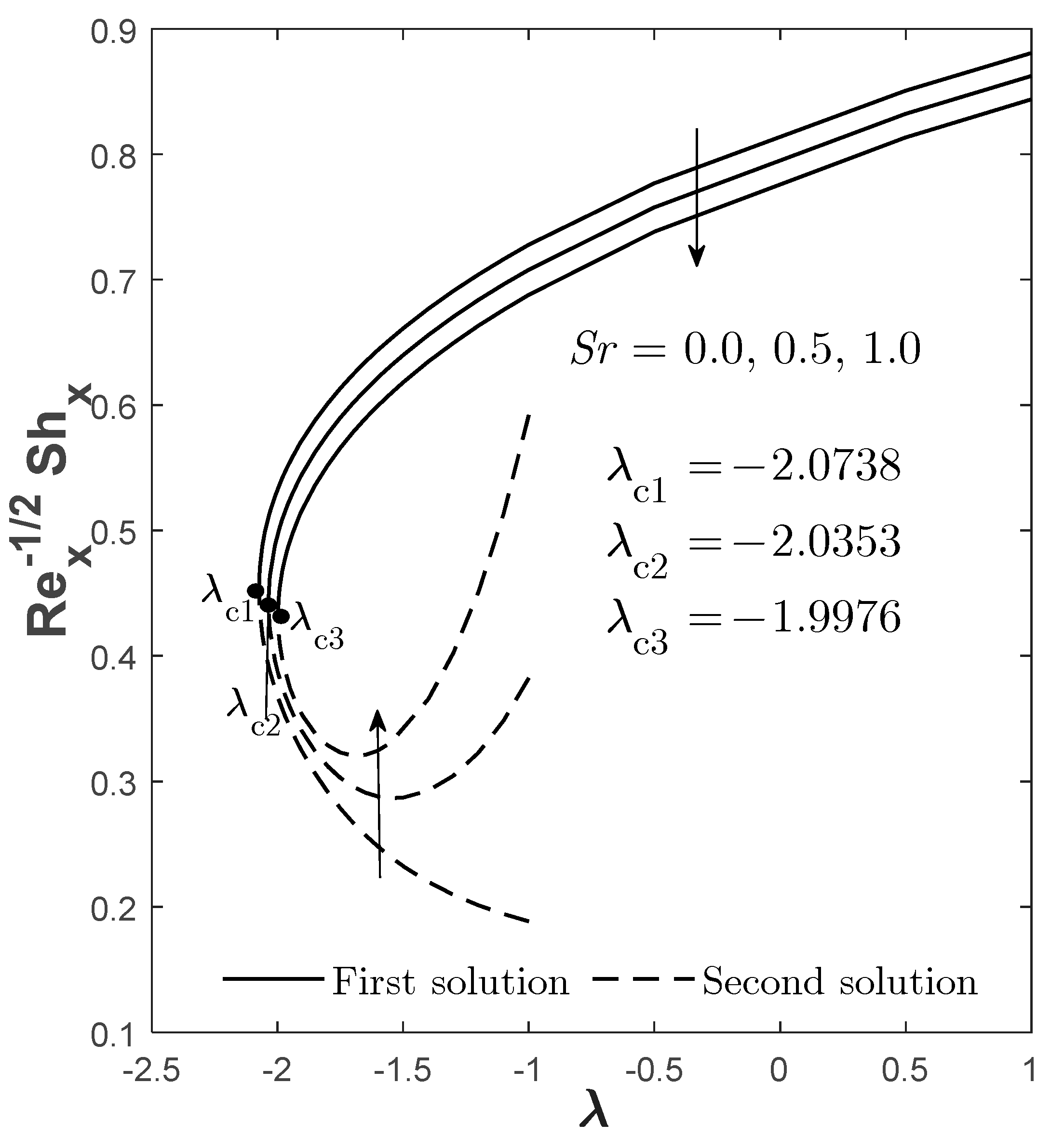
• Mass transfer rate is improvable by raising the volume fraction of copper and reducing the Soret effect.
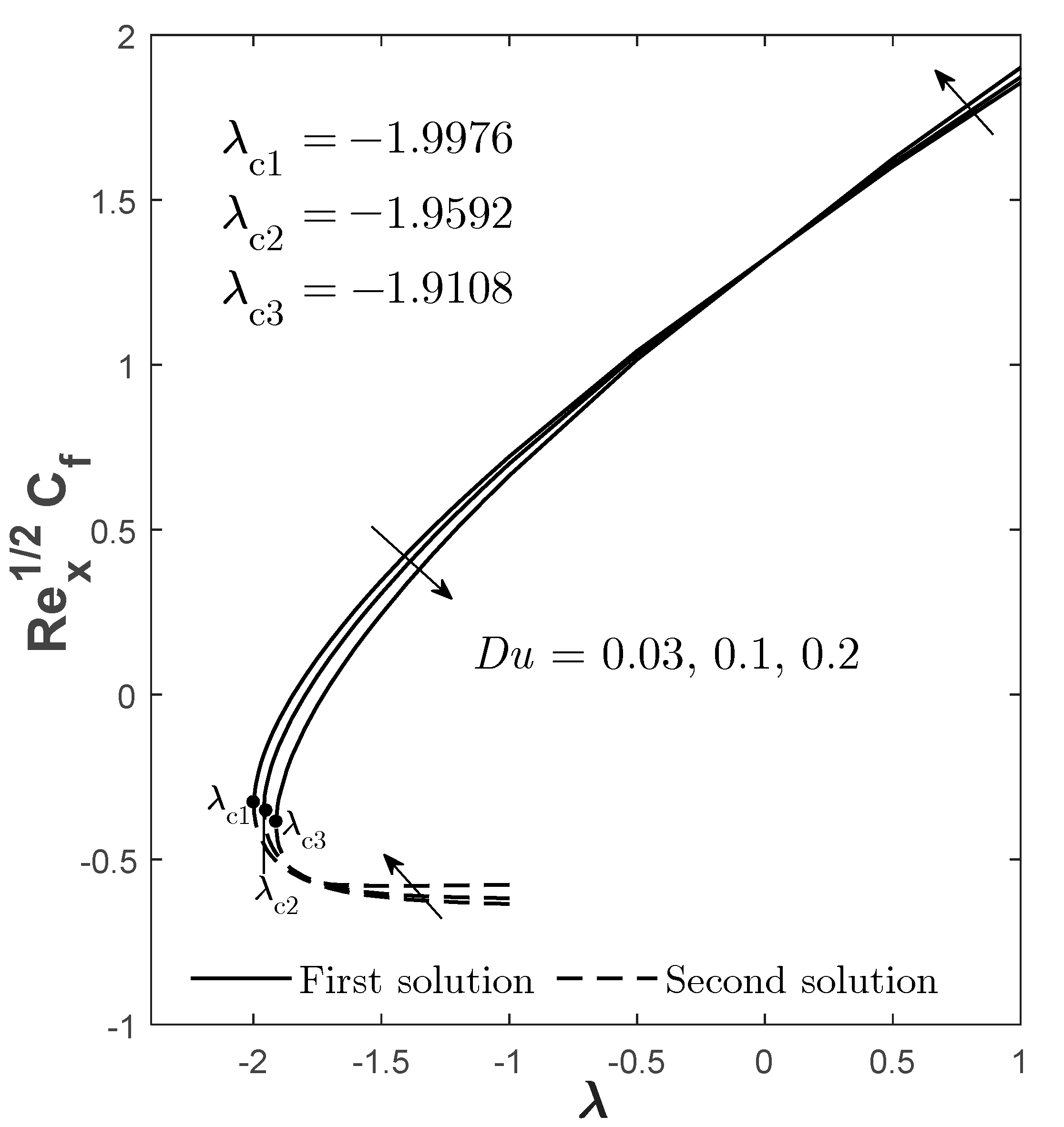
• The skin friction can be reduced by augmenting the Dufour and Soret effects during the opposing flow of mixed convection.
• The flow moves at a higher velocity when the hybrid nanofluid is concentrated but decelerated when stronger Dufour and Soret effects are inserted.
• The fluid temperature is reduceable by considering a greater copper volume fraction and Soret effect, thus, these two effects can be a coolant factor to the fluid.

However, these mentioned conclusions are specifically limited to the presented flow model. Different types of nanoparticle imposition and model geometries would lead to different findings. It is hoped that other researchers will benefit from these novel findings in determining the necessary factors to optimize the mass and heat transfer processes and identifying the proper parameters to execute all accessible solutions in controlling the flow.

References

1. Choi, S.U.S. Enhancing Thermal Conductivity of Fluids with Nanoparticles. In Proceedings of the Proceedings of the 1995 ASME International Mechanical Engineering Congress and Exposition, FED, San Francisco, CA, USA, 12–17 November 1995; Volume 231, pp. 99–106. [Google Scholar]
2. Buongiorno, J. Convective Transport in Nanofluids. J. Heat Transf. 2006, 128, 240–250. [Google Scholar] [CrossRef]
3. Tiwari, R.K.; Das, M.K. Heat Transfer Augmentation in a Two-Sided Lid-Driven Differentially Heated Square Cavity Utilizing Nanofluids. Int. J. Heat Mass Transf. 2007, 50, 2002–2018. [Google Scholar] [CrossRef]
4. Rizwana, R.; Hussain, A.; Nadeem, S. Mix Convection Non- Boundary Layer Flow of Unsteady MHD Oblique Stagnation Point Flow of Nanofluid. Int. Commun. Heat Mass Transf. 2021, 124, 105285. [Google Scholar] [CrossRef]
5. Ferdows, M.; Adesanya, S.O.; Alzahrani, F.; Yusuf, T.A. Numerical Investigation of a Boundary Layer Water-Based Nanofluid Flow with Induced Magnetic Field. Phys. Stat. Mech. Its Appl. 2021, 570, 125492. [Google Scholar] [CrossRef]
6. Swamy, H.A.K.; Sankar, M.; Reddy, N.K.; Manthari, M.S.A. Double Diffusive Convective Transport and Entropy Generation in an Annular Space Filled with Alumina-Water Nanoliquid. Eur. Phys. J. Spec. Top. 2022. [Google Scholar] [CrossRef]
7. Batool, S.; Rasool, G.; Alshammari, N.; Khan, I.; Kaneez, H.; Hamadneh, N. Numerical Analysis of Heat and Mass Transfer in Micropolar Nanofluids Flow through Lid Driven Cavity: Finite Volume Approach. Case Stud. Therm. Eng. 2022, 37, 102233. [Google Scholar] [CrossRef]
8. Sankar, M.; Swamy, H.A.K.; Do, Y.; Altmeyer, S. Thermal Effects of Nonuniform Heating in a Nanofluid-filled Annulus: Buoyant Transport versus Entropy Generation. Heat Transf. 2022, 51, 1062–1091. [Google Scholar] [CrossRef]
9. Suresh, S.; Venkitaraj, K.P.; Selvakumar, P.; Chandrasekar, M. Synthesis of Al2O3–Cu/Water Hybrid Nanofluids Using Two Step Method and Its Thermo Physical Properties. Colloids Surf. Physicochem. Eng. Asp. 2011, 388, 41–48. [Google Scholar] [CrossRef]
10. Suresh, S.; Venkitaraj, K.P.; Selvakumar, P.; Chandrasekar, M. Effect of Al2O3–Cu/Water Hybrid Nanofluid in Heat Transfer. Exp. Therm. Fluid Sci. 2012, 38, 54–60. [Google Scholar] [CrossRef]
11. Huminic, G.; Huminic, A. Hybrid Nanofluids for Heat Transfer Applications–A State-of-the-Art Review. Int. J. Heat Mass Transf. 2018, 125, 82–103. [Google Scholar] [CrossRef]
12. Chen, L.F.; Cheng, M.; Yang, D.J.; Yang, L. Enhanced Thermal Conductivity of Nanofluid by Synergistic Effect of Multi-Walled Carbon Nanotubes and Fe2O3 Nanoparticles. Appl. Mech. Mater. 2014, 548, 118–123. [Google Scholar] [CrossRef]
13. Selvakumar, P.; Suresh, S. Use of Al2O3-Cu/Water Hybrid Nanofluid in an Electronic Heat Sink. IEEE Trans. Compon. Packag. Manuf. Technol. 2012, 2, 1600–1607. [Google Scholar] [CrossRef]
14. Shenoy, A.; Sheremet, M.; Pop, I. Convective Flow and Heat Transfer from Wavy Surfaces: Viscous Fluids, Porous Media, and Nanofluids; CRC Press: Boca Raton, FL, USA; Taylor & Francis: Oxford, UK, 2016; a CRC title, part of the Taylor & Francis; ISBN 978-1-315-36763-7. [Google Scholar]
15. Merkin, J.H.; Pop, I.; Lok, Y.Y.; Groşan, T. Similarity Solutions for the Boundary Layer Flow and Heat Transfer of Viscous Fluids, Nanofluids, Porous Media, and Micropolar Fluids, 1st ed.; Elsevier: Oxford UK, 2021; ISBN 978-0-12-821188-5. [Google Scholar]
16. Abbas, N.; Malik, M.Y.; Nadeem, S. Stagnation Flow of Hybrid Nanoparticles with MHD and Slip Effects. Heat Transf.-Asian Res. 2019, 49, 180–196. [Google Scholar] [CrossRef]
17. Abbas, N.; Malik, M.Y.; Alqarni, M.S.; Nadeem, S. Study of Three Dimensional Stagnation Point Flow of Hybrid Nanofluid over an Isotropic Slip Surface. Phys. Stat. Mech. Its Appl. 2020, 554, 124020. [Google Scholar] [CrossRef]
18. Tulu, A.; Ibrahim, W. Effects of Second-Order Slip Flow and Variable Viscosity on Natural Convection Flow of CNTs−Fe3O4/Water Hybrid Nanofluids Due to Stretching Surface. Math. Probl. Eng. 2021, 2021, 8407194. [Google Scholar] [CrossRef]
19. Mahabaleshwar, U.S.; Vishalakshi, A.B.; Andersson, H.I. Hybrid Nanofluid Flow Past a Stretching/Shrinking Sheet with Thermal Radiation and Mass Transpiration. Chin. J. Phys. 2022, 75, 152–168. [Google Scholar] [CrossRef]
20. Khan, M.R.; Pan, K.; Khan, A.U.; Nadeem, S. Dual Solutions for Mixed Convection Flow of SiO2−Al2O3/Water Hybrid Nanofluid near the Stagnation Point over a Curved Surface. Phys. Stat. Mech. Its Appl. 2020, 547, 123959. [Google Scholar] [CrossRef]
21. Reddy, N.K.; Swamy, H.A.K.; Sankar, M. Buoyant Convective Flow of Different Hybrid Nanoliquids in a Non-Uniformly Heated Annulus. Eur. Phys. J. Spec. Top. 2021, 230, 1213–1225. [Google Scholar] [CrossRef]
22. Rastogi, R.P.; Madan, G.L. Dufour Effect in Liquids. J. Chem. Phys. 1965, 43, 4179–4180. [Google Scholar] [CrossRef]
23. Demirel, Y.; Gerbaud, V. Heat and Mass Transfer. In Nonequilibrium Thermodynamics; Elsevier: Amsterdam, The Netherlands, 2019; pp. 337–379. ISBN 978-0-444-64112-0. [Google Scholar]
24. Mortimer, R.G.; Eyring, H. Elementary Transition State Theory of the Soret and Dufour Effects. Proc. Natl. Acad. Sci. USA 1980, 77, 1728–1731. [Google Scholar] [CrossRef]
25. Seid, E.; Haile, E.; Walelign, T. Multiple Slip, Soret and Dufour Effects in Fluid Flow near a Vertical Stretching Sheet in the Presence of Magnetic Nanoparticles. Int. J. Thermofluids 2022, 13, 100136. [Google Scholar] [CrossRef]
26. Salleh, S.N.A.; Bachok, N.; Arifin, N.M.; Ali, F.M. Influence of Soret and Dufour on Forced Convection Flow towards a Moving Thin Needle Considering Buongiorno’s Nanofluid Model. Alex. Eng. J. 2020, 59, 3897–3906. [Google Scholar] [CrossRef]
27. Kumar, M.A.; Reddy, Y.D.; Goud, B.S.; Rao, V.S. Effects of Soret, Dufour, Hall Current and Rotation on MHD Natural Convective Heat and Mass Transfer Flow Past an Accelerated Vertical Plate through a Porous Medium. Int. J. Thermofluids 2021, 9, 100061. [Google Scholar] [CrossRef]
28. Jawad, M.; Saeed, A.; Kumam, P.; Shah, Z.; Khan, A. Analysis of Boundary Layer MHD Darcy-Forchheimer Radiative Nanofluid Flow with Soret and Dufour Effects by Means of Marangoni Convection. Case Stud. Therm. Eng. 2021, 23, 100792. [Google Scholar] [CrossRef]
29. Khan, A.A.; Abbas, N.; Nadeem, S.; Shi, Q.-H.; Malik, M.Y.; Ashraf, M.; Hussain, S. Non-Newtonian Based Micropolar Fluid Flow over Nonlinear Starching Cylinder under Soret and Dufour Numbers Effects. Int. Commun. Heat Mass Transf. 2021, 127, 105571. [Google Scholar] [CrossRef]
30. Salmi, A.; Madkhali, H.A.; Haneef, M.; Alharbi, S.O.; Malik, M.Y. Numerical Study on Thermal Enhancement in Magnetohydrodynamic Micropolar Liquid Subjected to Motile Gyrotactic Microorganisms Movement and Soret and Dufour Effects. Case Stud. Therm. Eng. 2022, 35, 102090. [Google Scholar] [CrossRef]
31. Yinusa, A.A.; Sobamowo, M.G.; Usman, M.A.; Abubakar, E.H. Exploration of Three Dimensional Squeezed Flow and Heat Transfer through a Rotating Channel with Coupled Dufour and Soret Influences. Therm. Sci. Eng. Prog. 2021, 21, 100788. [Google Scholar] [CrossRef]
32. Pal, D.; Das, B.C.; Vajravelu, K. Magneto-Soret-Dufour Thermo-Radiative Double-Diffusive Convection Heat and Mass Transfer of a Micropolar Fluid in a Porous Medium with Ohmic Dissipation and Variable Thermal Conductivity. Propuls. Power Res. 2022, 11, 154–170. [Google Scholar] [CrossRef]
33. Sheri, S.R.; Megaraju, P.; Rajashekar, M.N. Impact of Hall Current, Dufour and Soret on Transient MHD Flow Past an Inclined Porous Plate: Finite Element Method. Mater. Today Proc. 2022, 59, 1009–1021. [Google Scholar] [CrossRef]
34. Srinivasacharya, D.; RamReddy, C. Soret and Dufour Effects on Mixed Convection from an Exponentially Stretching Surface. Int. J. Nonlinear Sci. 2011, 12, 60–68. [Google Scholar]
35. Takabi, B.; Salehi, S. Augmentation of the Heat Transfer Performance of a Sinusoidal Corrugated Enclosure by Employing Hybrid Nanofluid. Adv. Mech. Eng. 2015, 6, 147059. [Google Scholar] [CrossRef]
36. Oztop, H.F.; Abu-Nada, E. Numerical Study of Natural Convection in Partially Heated Rectangular Enclosures Filled with Nanofluids. Int. J. Heat Fluid Flow 2008, 29, 1326–1336. [Google Scholar] [CrossRef]
37. Jamil, F.; Ali, H.M. Applications of Hybrid Nanofluids in Different Fields. In Hybrid Nanofluids for Convection Heat Transfer; Elsevier: Amsterdam, The Netherlands, 2020; pp. 215–254. ISBN 978-0-12-819280-1. [Google Scholar]
38. Brimmo, A.T.; Qasaimeh, M.A. Stagnation Point Flows in Analytical Chemistry and Life Sciences. RSC Adv. 2017, 7, 51206–51232. [Google Scholar] [CrossRef]
39. Tadmor, Z.; Klein, I. Engineering Principles of Plasticating Extrusion; Polymer Science and Engineering Series; Van Nostrand Reinhold Co.: New York, NY, USA, 1970. [Google Scholar]
40. Kuznetsov, A.V.; Nield, D.A. Natural Convective Boundary-Layer Flow of a Nanofluid Past a Vertical Plate. Int. J. Therm. Sci. 2010, 49, 243–247. [Google Scholar] [CrossRef]
41. Turkyilmazoglu, M. Single Phase Nanofluids in Fluid Mechanics and Their Hydrodynamic Linear Stability Analysis. Comput. Methods Programs Biomed. 2020, 187, 105171. [Google Scholar] [CrossRef]
42. Bhattacharyya, K.; Layek, G.C.; Seth, G.S. Soret and Dufour Effects on Convective Heat and Mass Transfer in Stagnation-Point Flow towards a Shrinking Surface. Phys. Scr. 2014, 89, 095203. [Google Scholar] [CrossRef]
43. Mohamed, M.K.A.; Salleh, M.Z.; Nazar, R.; Ishak, A. Numerical Investigation of Stagnation Point Flow over a Stretching Sheet with Convective Boundary Conditions. Bound. Value Probl. 2013, 2013, 4. [Google Scholar] [CrossRef]
44. Zainal, N.A.; Nazar, R.; Naganthran, K.; Pop, I. MHD Mixed Convection Stagnation Point Flow of a Hybrid Nanofluid Past a Vertical Flat Plate with Convective Boundary Condition. Chin. J. Phys. 2020, 66, 630–644. [Google Scholar] [CrossRef]
45. Prasad, K.V.; Vajravelu, K.; Vaidya, H.; Santhi, S.R. Axisymmetric Flow of a Nanofluid Past a Vertical Slender Cylinder in the Presence of a Transverse Magnetic Field. J. Nanofluids 2016, 5, 101–109. [Google Scholar] [CrossRef]
46. Devi, S.U.; Devi, S.A. Heat Transfer Enhancement of Cu-Al2O3/Water Hybrid Nanofluid Flow over a Stretching Sheet. J. Niger. Math. Soc. 2017, 36, 419–433. [Google Scholar]
47. Rosseland, S. Astrophysik auf atomtheoretischer Grundlage; Springer: Berlin, Germany, 1931; ISBN 978-3-662-26679-3. [Google Scholar]
48. Cortell Bataller, R. Radiation Effects in the Blasius Flow. Appl. Math. Comput. 2008, 198, 333–338. [Google Scholar] [CrossRef]
49. Magyari, E.; Pantokratoras, A. Note on the Effect of Thermal Radiation in the Linearized Rosseland Approximation on the Heat Transfer Characteristics of Various Boundary Layer Flows. Int. Commun. Heat Mass Transf. 2011, 38, 554–556. [Google Scholar] [CrossRef]
50. Bilal Ashraf, M.; Hayat, T.; Alsaedi, A.; Shehzad, S.A. Soret and Dufour Effects on the Mixed Convection Flow of an Oldroyd-B Fluid with Convective Boundary Conditions. Results Phys. 2016, 6, 917–924. [Google Scholar] [CrossRef]
51. Tai, B.-C.; Char, M.-I. Soret and Dufour Effects on Free Convection Flow of Non-Newtonian Fluids along a Vertical Plate Embedded in a Porous Medium with Thermal Radiation. Int. Commun. Heat Mass Transf. 2010, 37, 480–483. [Google Scholar] [CrossRef]
52. Asghar, A.; Lund, L.A.; Shah, Z.; Vrinceanu, N.; Deebani, W.; Shutaywi, M. Effect of Thermal Radiation on Three-Dimensional Magnetized Rotating Flow of a Hybrid Nanofluid. Nanomaterials 2022, 12, 1566. [Google Scholar] [CrossRef]
53. Gumber, P.; Yaseen, M.; Rawat, S.K.; Kumar, M. Heat Transfer in Micropolar Hybrid Nanofluid Flow Past a Vertical Plate in the Presence of Thermal Radiation and Suction/Injection Effects. Partial Differ. Equ. Appl. Math. 2022, 5, 100240. [Google Scholar] [CrossRef]
54. Merkin, J.H. On Dual Solutions Occurring in Mixed Convection in a Porous Medium. J. Eng. Math. 1986, 20, 171–179. [Google Scholar] [CrossRef]
55. Weidman, P.D.; Kubitschek, D.G.; Davis, A.M.J. The Effect of Transpiration on Self-Similar Boundary Layer Flow over Moving Surfaces. Int. J. Eng. Sci. 2006, 44, 730–737. [Google Scholar] [CrossRef]
56. Harris, S.D.; Ingham, D.B.; Pop, I. Mixed Convection Boundary-Layer Flow Near the Stagnation Point on a Vertical Surface in a Porous Medium: Brinkman Model with Slip. Transp. Porous Media 2009, 77, 267–285. [Google Scholar] [CrossRef]
57. Kierzenka, J.; Shampine, L.F. A BVP Solver Based on Residual Control and the Maltab PSE. ACM Trans. Math. Softw. 2001, 27, 299–316. [Google Scholar] [CrossRef]
58. Shampine, L.F.; Gladwell, I.; Thompson, S. Solving ODEs with MATLAB, 1st ed.; Cambridge University Press: Cambridge, UK, 2003; ISBN 978-0-521-82404-0. [Google Scholar]
59. Khashi’ie, N.S.; Md Arifin, N.; Pop, I. Mixed Convective Stagnation Point Flow towards a Vertical Riga Plate in Hybrid Cu-Al2O3/Water Nanofluid. Mathematics 2020, 8, 912. [Google Scholar] [CrossRef]
60. Wahid, N.S.; Arifin, N.M.; Khashi’ie, N.S.; Pop, I.; Bachok, N.; Hafidzuddin, M.E.H. Unsteady Mixed Convective Stagnation Point Flow of Hybrid Nanofluid in Porous Medium. Neural Comput. Appl. 2022, 34, 14699–14715. [Google Scholar] [CrossRef]
61. Ishak, A.; Nazar, R.; Bachok, N.; Pop, I. MHD Mixed Convection Flow near the Stagnation-Point on a Vertical Permeable Surface. Phys. Stat. Mech. Its Appl. 2010, 389, 40–46. [Google Scholar] [CrossRef]
62. Roşca, A.V.; Roşca, N.C.; Pop, I. Mixed Convection Stagnation Point Flow of a Hybrid Nanofluid Past a Vertical Flat Plate with a Second Order Velocity Model. Int. J. Numer. Methods Heat Fluid Flow 2021, 31, 75–91. [Google Scholar] [CrossRef]
63. Ramachandran, N.; Chen, T.S.; Armaly, B.F. Mixed Convection in Stagnation Flows Adjacent to Vertical Surfaces. J. Heat Transf. 1988, 110, 373–377. [Google Scholar] [CrossRef]
64. Brinkman, H.C. The Viscosity of Concentrated Suspensions and Solutions. J. Chem. Phys. 1952, 20, 571. [Google Scholar] [CrossRef]
Figure 1. Physical model.
Mathematics 10 02966 g001
Figure 2. Re x 1 / 2 C f for varied ϕ 2 when N = R d = S c = S r = 1 , D u = 0.03 , and B i = 0.1 .
Mathematics 10 02966 g002
Figure 3. Re x 1 / 2 N u x for varied ϕ 2 when N = R d = S c = S r = 1 , D u = 0.03 , and B i = 0.1 .
Mathematics 10 02966 g003
Figure 4. Re x 1 / 2 S h x for varied ϕ 2 when N = R d = S c = S r = 1 , D u = 0.03 , and B i = 0.1 .
Mathematics 10 02966 g004
Figure 5. Re x 1 / 2 C f for varied D u when N = R d = S c = S r = 1 , ϕ 2 = 0.01 , and B i = 0.1 .
Mathematics 10 02966 g005
Figure 6. Re x 1 / 2 N u x for varied D u when N = R d = S c = S r = 1 , ϕ 2 = 0.01 , and B i = 0.1 .
Mathematics 10 02966 g006
Figure 7. Re x 1 / 2 S h x for varied D u when N = R d = S c = S r = 1 , ϕ 2 = 0.01 , and B i = 0.1 .
Mathematics 10 02966 g007
Figure 8. Re x 1 / 2 C f for varied S r when N = R d = S c = 1 , ϕ 2 = 0.01 , D u = 0.03 , and B i = 0.1 .
Mathematics 10 02966 g008
Figure 9. Re x 1 / 2 N u x for varied S r when N = R d = S c = 1 , ϕ 2 = 0.01 , D u = 0.03 , and B i = 0.1 .
Mathematics 10 02966 g009
Figure 10. Re x 1 / 2 S h x for varied S r when N = R d = S c = 1 , ϕ 2 = 0.01 , D u = 0.03 , and B i = 0.1 .
Mathematics 10 02966 g010
Figure 11. Plots of f η for varied ϕ 2 when N = R d = S c = S r = 1 , λ = 1 , D u = 0.03 , and B i = 0.1 .
Mathematics 10 02966 g011
Figure 12. Plots of θ η for varied ϕ 2 when N = R d = S c = S r = 1 , λ = 1 , D u = 0.03 , and B i = 0.1 .
Mathematics 10 02966 g012
Figure 13. Plots of h η for varied ϕ 2 when N = R d = S c = S r = 1 , λ = 1 , D u = 0.03 , and B i = 0.1 .
Mathematics 10 02966 g013
Figure 14. Plots of f η for varied D u when N = R d = S c = S r = 1 , λ = 1 , ϕ 2 = 0.01 , and B i = 0.1 .
Mathematics 10 02966 g014
Figure 15. Plots of θ η for varied D u when N = R d = S c = S r = 1 , λ = 1 , ϕ 2 = 0.01 , and B i = 0.1 .
Mathematics 10 02966 g015
Figure 16. Plots of h η for varied D u when N = R d = S c = S r = 1 , λ = 1 , ϕ 2 = 0.01 , and B i = 0.1 .
Mathematics 10 02966 g016
Figure 17. Plots of f η for varied S r when N = R d = S c = 1 , D u = 0.03 , λ = 1 , ϕ 2 = 0.01 , and B i = 0.1 .
Mathematics 10 02966 g017
Figure 18. Plots of θ η for varied S r when N = R d = S c = 1 , D u = 0.03 , λ = 1 , ϕ 2 = 0.01 , and B i = 0.1 .
Mathematics 10 02966 g018
Figure 19. Plots of h η for varied S r when N = R d = S c = 1 , D u = 0.03 , λ = 1 , B i = 0.1 , and ϕ 2 = 0.01 .
Mathematics 10 02966 g019
Figure 20. Plots of γ 1 for selected λ c when N = R d = S c = S r = 1 , ϕ 2 = 0.01 , D u = 0.03 , and B i = 0.1 .
Mathematics 10 02966 g020