An Approximate Proximal Numerical Procedure Concerning the Generalized Method of Lines

Abstract

This article develops an approximate proximal approach for the generalized method of lines. We recall that for the generalized method of lines, the domain of the partial differential equation in question is discretized in lines (or in curves) and the concerning solution is developed on these lines, as functions of the boundary conditions and the domain boundary shape. Considering such a context, in the text we develop an approximate numerical procedure of proximal nature applicable to a large class of models in physics and engineering. Finally, in the last sections, we present numerical examples and results related to a Ginzburg–Landau-type equation.

1. Introduction

We start by recalling that the generalized method of lines was originally introduced in the book entitled “Topics on Functional Analysis, Calculus of Variations and Duality” [1], published in 2011.

Indeed, the present results are extensions and applications of previous ones, which have been published since 2011, in books and articles such as [1,2,3,4]. About the Sobolev spaces involved, we would mention [5,6]. Concerning the applications, related models in physics are addressed in [7,8].

We also emphasize that, in such a method, the domain of the partial differential equation in question is discretized in lines (or more generally, in curves), and the concerning solution is written on these lines as functions of boundary conditions and the domain boundary shape.

In fact, in its previous format, this method consists of an application of a kind of a partial finite differences procedure combined with the Banach fixed point theorem to obtain the relation between two adjacent lines (or curves).

In the present article, we propose an approximate approach and a related iterative procedure of proximal nature. We highlight that this is a proximal method inspired by some models concerning duality principles in D.C optimization in the calculus of variations, such as those found in Toland [9].

In the next lines and sections we develop in detail such a numerical procedure.

With such statements in mind, let $\mathrm{\Omega }\subset {\mathbb{R}}^2$ be an open, bounded and connected set where:

$$\mathrm{\Omega }=\{(x,y)\in {\mathbb{R}}^2:y_1\left(x\right)\le y\le y_2\left(x\right),a\le x\le b\}.$$

Here, we assume, $y_1,y_2:[a,b]\to \mathbb{R}$ are continuous functions.

Consider the Ginzburg–Landau-type equation, defined by:

$$\left\{\begin{array}{cc}-\epsilon {\nabla }^{2}u+\alpha u^3-\beta u=f,\hfill & \mathrm{in}\mathrm{\Omega },\hfill \\ u=0,\hfill & \mathrm{on}\partial \mathrm{\Omega },\hfill \end{array}\right.$$

(1)

where $\epsilon >0$, $\alpha >0,\beta >0$ and $f\in L^2(\mathrm{\Omega })$.

Furthermore, $u\in W_0^{1,2}(\mathrm{\Omega })$, and the equation in question must be considered in a distributional sense.

In the next section, we address the problem of approximately solving this concerning equation. We highlight that the methods and ideas exposed are applicable to a large class of similar models in physics and engineering.

2. The Numerical Method

We discretize the interval $[a,b]$ into N same measure sub-intervals, through a partition

$$P=\{x_0=a,x_1,\cdots ,x_N=b\},$$

where $x_n=a+nd,\forall n\in \{1,\cdots ,N-1\}.$ Here,

$$d=\frac{(b-a)}{N}.$$

Through such a procedure, we generate N vertical lines parallel to the Cartesian axis $0y$, so that for each line n, based on the point $x_n$, we are going to compute an approximate solution $u_n\left(y\right)$ corresponding to values of u on such a line.

Considering this procedure, the equation system obtained in partial finite differences (please see [10], for concerning models in finite differences) is given by:

$$-\epsilon \left(\frac{u_{n+1}-2u_n+u_{n-1}}{d^2}+\frac{{\partial }^2{u}_n}{\partial y^2}\right)+\alpha u_n^3-\beta u_n=f_n,$$

$\forall n\in \{1,\cdots ,N-1\},$ with the boundary conditions:

$$u_0=0,$$

and,

$$u_N=0.$$

Let $K>0$ be an appropriate constant to be specified.

In a proximal approach, considering an initial solution:

$$\left\{{\left(u_0\right)}_n\right\},$$

we redefine the system of equations in question as below indicated.

$$-\epsilon \left(\frac{u_{n+1}-2u_n+u_{n-1}}{d^2}+\frac{{\partial }^2{u}_n}{\partial y^2}\right)+\alpha u_n^3-\beta u_n+K{u}_n-K{\left(u_0\right)}_n=f_n,$$

$\forall n\in \{1,\cdots ,N-1\},$ with the boundary conditions:

$$u_0=0,$$

and,

$$u_N=0.$$

Hence, we may denote:

$$u_{n+1}-\left(2+K\frac{d^2}{\epsilon }\right)u_n+u_{n-1}+T\left(u_n\right)+{\tilde{f}}_n\frac{d^2}{\epsilon }=0,$$

where,

$$T\left(u_n\right)=\left(-\alpha u_n^3+\beta u_n\right)\frac{d^2}{\epsilon }+\frac{{\partial }^2{u}_n}{\partial y^2}{d}^2,$$

and ${\tilde{f}}_n=K{\left(u_0\right)}_n+f_n,$$\forall n\in \{1,\cdots ,N-1\}.$

In particular, for $n=1$, we obtain:

$$u_2-\left(2+K\frac{d^2}{\epsilon }\right)u_1+T\left(u_1\right)+{\tilde{f}}_1\frac{d^2}{\epsilon }=0,$$

so that,

$$u_1=a_1{u}_2+b_{1}T\left(u_2\right)+c_1+E_1,$$

where,

$$a_1=\frac{1}{2+K\frac{d^2}{\epsilon }},$$

$$b_1=a_1,$$

and,

$$c_1=a_1\widetilde{f_1}\frac{d^2}{\epsilon }$$

and the error $E_1$, proportional to $1/K$, is given by:

$$E_1=b_1(T\left(u_1\right)-T\left(u_2\right)).$$

Now, reasoning inductively, having,

$$u_{n-1}=a_{n-1}{u}_n+b_{n-1}T\left(u_n\right)+c_{n-1}+E_{n-1}$$

for the line n, we have,

$$\begin{array}{ccc}& & u_{n+1}-\left(2+K\frac{d^2}{\epsilon }\right)u_n+a_{n-1}{u}_n+b_{n-1}T\left(u_n\right)+c_{n-1}+E_{n-1}\hfill \\ & & +T\left(u_n\right)+{\tilde{f}}_n\frac{d^2}{\epsilon }=0,\hfill \end{array}$$

(2)

so that,

$$u_n=a_n{u}_{n+1}+b_{n}T\left(u_{n+1}\right)+c_n+E_n,$$

where,

$$a_n=\frac{1}{2+K\frac{d^2}{\epsilon }-a_{n-1}},$$

$$b_n=a_n(b_{n-1}+1),$$

and,

$$c_n=a_n\left(c_{n-1}+{\tilde{f}}_n\frac{d^2}{\epsilon }\right)$$

and the error $E_n$, is given by:

$$E_n=a_n{E}_{n-1}+b_n(T\left(u_n\right)-T\left(u_{n+1}\right)),$$

$\forall n\in \{1,\cdots ,N-1\}.$

In particular, for $n=N-1$, we have $u_N=0$ so that,

$$\begin{array}{ccc}\hfill u_{N-1}& \approx & a_{N-1}{u}_N+b_{N-1}T\left(u_N\right)+c_{N-1}\hfill \\ & \approx & a_{N-1}{u}_N+b_{N-1}\frac{{\partial }^2{u}_{N-1}}{\partial y^2}{d}^2+b_{N-1}(-\alpha u_N^3+\beta u_N)\frac{d^2}{\epsilon }+c_{N-1}\hfill \\ & =& b_{N-1}\frac{{\partial }^2{u}_{N-1}}{\partial y^2}{d}^2+c_{N-1}.\hfill \end{array}$$

(3)

This last equation is an ODE from which we may easily obtain $u_{N-1}$ with the boundary conditions

$$u_{N-1}\left(y_1\left(x_{N-1}\right)\right)=u_{N-1}\left(y_2\left(x_{N-1}\right)\right)=0.$$

Having $u_{N-1}$, we may obtain $u_{N-2}$ though the equation:

$$\begin{array}{ccc}\hfill u_{N-2}& \approx & a_{N-2}{u}_{N-1}+b_{N-2}T\left(u_{N-1}\right)+c_{N-2}\hfill \\ & \approx & a_{N-2}{u}_{N-1}+b_{N-2}\frac{{\partial }^2{u}_{N-2}}{\partial y^2}{d}^2+b_{N-2}(-\alpha u_{N-1}^3+\beta u_{N-1})\frac{d^2}{\epsilon }+c_{N-2},\hfill \end{array}$$

(4)

with the boundary conditions:

$$u_{N-2}\left(y_1\left(x_{N-2}\right)\right)=u_{N-2}\left(y_2\left(x_{N-2}\right)\right)=0.$$

And so on, up to finding $u_1.$

The next step is to replace $\left\{{\left(u_0\right)}_n\right\}$ by $\left\{u_n\right\}$ and then to repeat the process until an appropriate convergence criterion is satisfied.

The problem is then approximately solved.

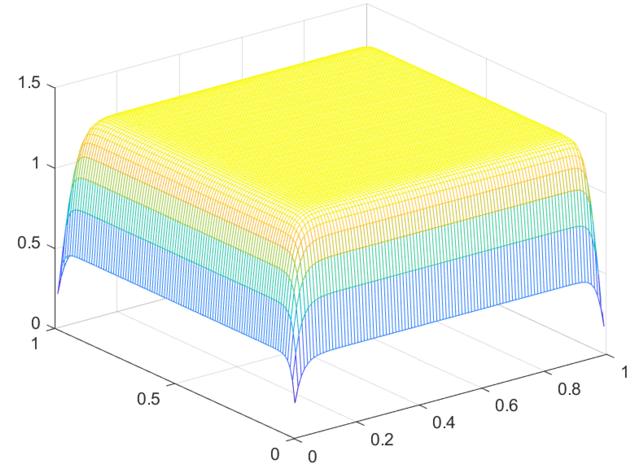
3. A Numerical Example

We present numerical results for $\mathrm{\Omega }=[0,1]\times [0,1],$$\alpha =\beta =1$, $f\equiv 1$ in $\mathrm{\Omega }$, $N=100$, $K=50$ and for:

$$\epsilon =0.1,0.01\mathrm{and}0.001.$$

For such values of $\epsilon$, please see Figure 1, Figure 2 and Figure 3, respectively.

Remark 1.

We observe that as $\epsilon >0$ decreases to the value $0.001$, the solution approaches the constant value $1.3247$ along the domain, up to the satisfaction of boundary conditions. This is expected, since this value is an approximate solution of equation $u^3-u-1=0.$

4. A General Proximal Explicit Approach

Based on the algorithm presented in the last section, we develop a software in MATHEMATICA in order to approximately solve the following equation.

$$\left\{\begin{array}{cc}-\epsilon \left(\frac{{\partial }^{2}u}{\partial r^2}+\frac{1}{r}\frac{\partial u}{\partial r}+\frac{1}{r^2}\frac{{\partial }^{2}u}{\partial {\theta }^2}\right)+\alpha u^3-\beta u=f,\hfill & \mathrm{in}\mathrm{\Omega },\hfill \\ u=0,\hfill & \mathrm{on}\partial {\mathrm{\Omega }}_1,\hfill \\ u=u_f\left(\theta \right),\hfill & \mathrm{on}\partial {\Gamma }_2.\hfill \end{array}\right.$$

(5)

Here:

$$\mathrm{\Omega }=\{(r,\theta )\in {\mathbb{R}}^2:1\le r\le 2,0\le \theta \le 2\pi \},$$

$$\partial {\mathrm{\Omega }}_1=\{(1,\theta )\in {\mathbb{R}}^2:0\le \theta \le 2\pi \},$$

$$\partial {\mathrm{\Omega }}_2=\{(2,\theta )\in {\mathbb{R}}^2:0\le \theta \le 2\pi \},$$

$\alpha =\beta =1$, $K=10$, $N=100$ and $f\equiv 1,\mathrm{on}\mathrm{\Omega }.$

At this point we present such a software in MATHEMATICA.

******************************************

• $m8=100;$
• $d=1.0/m8;$
• $K=10.0;$
• $e1=0.01;$
• $A=1.0;$
• $B=1.0;$
• For[i = 1, i < m8 + 1, i++,
  uo[i] = 0.0];
• For[k = 1, k < 150, k++,
  Print[k];
  a[1] = 1/(2.0 + $K*d^2/e1$);
  b[1] = a[1];
  c[1] = a[1]*(K*uo[1] + 1.0)*$d^2/e1$;
  For[i = 2, i < m8, i++,
  a[i] = $1/(2.0+K*d^2/e1-a[i-1]);$
  b[i] = a[i]*(b[i - 1] + 1);
  c[i] = a[i]*(c[i - 1] + $(K*uo\left[i\right]+1.0)*d^2/e1)$];
• u[m8] = uf[x]; d1 = 1.0;
• For[i = 1, i < m8, i++,
  t[m8 - i] = 1 + (m8 - i)*d;
  A1 = (a[m8 - i]*u[m8 - i + 1] +
  b[m8 - i]*(-A*$u{[m8-i+1]}^3$ + B*u[m8 - i + 1])*$d^2/e1*d{1}^2$ +
  c[m8 - i] +
  $d^2*d{1}^2$*b[m8 - i]*(D[u[m8 - i + 1], x, 2]/$t{[m8-i]}^2$) +
  $d{1}^2*1/t[m8-i]$*b[m8 - i]* $d^2$ (uo[m8 - i + 1] - uo[m8 - i])/d)/(1.0);
  A1 = Expand[A1];
  A1 = Series[ A1, {uf[x], 0, 3}, {uf’[x], 0, 1}, {uf”[x], 0, 1}, {uf”’[x], 0, 0}, {uf””[x], 0, 0}];
  A1 = Normal[A1];
  u[m8 - i] = Expand[A1]];
  For[i = 1, i < m8 + 1, i++,
  uo[i] = u[i]]; d1 = 1.0;
  Print[Expand[u[m8/2]]]]

************************************

For such a general approach, for $\epsilon =0.1$, we have obtained the following lines (here x stands for $\theta$).

$$\begin{array}{ccc}\hfill u\left[10\right]\left(x\right)& =& 0.4780+0.0122u_f\left[x\right]-0.0115u_f{\left[x\right]}^2+0.0083u_f{\left[x\right]}^3+0.00069u_f^{\prime \prime }\left[x\right]\hfill \\ & & -0.0014u_f\left[x\right]\left(u_f^{\prime \prime }\right)\left[x\right]+0.0016uf{\left[x\right]}^2{u}_f^{\prime \prime }\left[x\right]-0.00092u_f{\left[x\right]}^3{u}_f^{\prime \prime }\left[x\right]\hfill \end{array}$$

(6)

$$\begin{array}{ccc}\hfill u\left[20\right]\left(x\right)& =& 0.7919+0.0241u_f\left[x\right]-0.0225u_f{\left[x\right]}^2+0.0163u_f{\left[x\right]}^3+0.0012u_f^{\prime \prime }\left[x\right]\hfill \\ & & -0.0025u_f\left[x\right]\left(u_f^{\prime \prime }\right)\left[x\right]+0.0030u_f{\left[x\right]}^2\left(u_f^{\prime \prime }\right)\left[x\right]-0.0018u_f{\left[x\right]}^3\left(u_f^{\prime \prime }\right)\left[x\right].\hfill \end{array}$$

(7)

$$\begin{array}{ccc}\hfill u\left[30\right]\left(x\right)& =& 0.9823+0.0404u_f\left[x\right]-0.0375u_f{\left[x\right]}^2+0.0266u_f{\left[x\right]}^3+0.00180\left(u_f^{\prime \prime }\right)\left[x\right]\hfill \\ & & -0.00362u_f\left[x\right]\left(u_f^{\prime \prime }\right)\left[x\right]+0.0043u_f{\left[x\right]}^2\left(u{f}^{\prime \prime }\right)\left[x\right]-0.0028u_f{\left[x\right]}^3\left(u{f}^{\prime \prime }\right)\left[x\right]\hfill \end{array}$$

(8)

$$\begin{array}{ccc}\hfill u\left[40\right]\left(x\right)& =& 1.0888+0.0698u_f\left[x\right]-0.0632u_f{\left[x\right]}^2+0.0433u_f{\left[x\right]}^3+0.0026\left(u_f^{\prime \prime }\right)\left[x\right]\hfill \\ & & -0.0051u_f\left[x\right]\left(u_f^{\prime \prime }\right)\left[x\right]+0.0061u_f{\left[x\right]}^2\left(u_f^{\prime \prime }\right)\left[x\right]-0.0043u_f{\left[x\right]}^3\left(u_f^{\prime \prime }\right)\left[x\right]\hfill \end{array}$$

(9)

$$\begin{array}{ccc}\hfill u\left[50\right]\left(x\right)& =& 1.1316+0.1277u_f\left[x\right]-0.1101u_f{\left[x\right]}^2+0.0695u_f{\left[x\right]}^3+0.0037\left(u_f^{\prime \prime }\right)\left[x\right]\hfill \\ & & -0.0073u_f\left[x\right]\left(u_f^{\prime \prime }\right)\left[x\right]+0.0084u_f{\left[x\right]}^2\left(u_f^{\prime \prime }\right)\left[x\right]-0.0062u_f{\left[x\right]}^3\left(u_f^{\prime \prime }\right)\left[x\right]\hfill \end{array}$$

(10)

$$\begin{array}{ccc}\hfill u\left[60\right]\left(x\right)& =& 1.1104+0.2389u_f\left[x\right]-0.1866u_f{\left[x\right]}^2+0.0988u_f{\left[x\right]}^3+0.0053\left(u_f^{\prime \prime }\right)\left[x\right]\hfill \\ & & -0.0099u_f\left[x\right]\left(u_f^{\prime \prime }\right)\left[x\right]+0.0105u_f{\left[x\right]}^2\left(u_f^{\prime \prime }\right)\left[x\right]-0.0075u_f{\left[x\right]}^3\left(u_f^{\prime \prime }\right])\left[x\right]\hfill \end{array}$$

(11)

$$\begin{array}{ccc}\hfill u\left[70\right]\left(x\right)& =& 1.0050+0.4298u_f\left[x\right]-0.273813u_f{\left[x\right]}^2+0.0949u_f{\left[x\right]}^3+0.0070\left(u_f^{\prime \prime }\right)\left[x\right]\hfill \\ & & -0.0116u_f\left[x\right]\left(u_f^{\prime \prime }\right)\left[x\right]+0.0102u_f{\left[x\right]}^2\left(u_f^{\prime \prime }\right)\left[x\right]-0.0061u_f{\left[x\right]}^3\left(u_f^{\prime \prime }\right)\left[x\right]\hfill \end{array}$$

(12)

$$\begin{array}{ccc}\hfill u\left[80\right]\left(x\right)& =& 0.7838+0.6855u_f\left[x\right]-0.2892u_f{\left[x\right]}^2+0.0161u_f{\left[x\right]}^3+0.0075\left(u_f^{\prime \prime }\right)\left[x\right]\hfill \\ & & -0.0098u_f\left[x\right]\left(u_f^{\prime \prime }\right)\left[x\right]+0.0063084uf{\left[x\right]}^2\left(u{f}^{\prime \prime }\right)\left[x\right]-0.0027u_f{\left[x\right]}^3\left(u_f^{\prime \prime }\right)\left[x\right]\hfill \end{array}$$

(13)

$$\begin{array}{ccc}\hfill u\left[90\right]\left(x\right)& =& 0.4359+0.9077u_f\left[x\right]-0.1621u_f{\left[x\right]}^2-0.0563u_f{\left[x\right]}^3+0.0051\left(u_f^{\prime \prime }\right)\left[x\right]\hfill \\ & & -0.0047u_f\left[x\right]\left(u_f^{\prime \prime }\right)\left[x\right]+0.0023u_f{\left[x\right]}^2\left(u_f^{\prime \prime }\right)\left[x\right]-0.00098u_f{\left[x\right]}^3\left(u_f^{\prime \prime }\right)\left[x\right]\hfill \end{array}$$

(14)

For $\epsilon =0.01$, we have obtained the following line expressions.

$$\begin{array}{ccc}\hfill u\left[10\right]\left(x\right)& =& 1.0057+2.07*{10}^{-11}{u}_f\left[x\right]-1.85*{10}^{-11}{u}_f{\left[x\right]}^2+1.13*{10}^{-11}{u}_f{\left[x\right]}^3\hfill \\ & & +4.70*{10}^{-13}\left(u_f^{\prime \prime }\right)\left[x\right]-8.44*{10}^{-13}{u}_f\left[x\right]\left(u_f^{\prime \prime }\right)\left[x\right]\hfill \\ & & +7.85*{10}^{-13}{u}_f{\left[x\right]}^2\left(u_f^{\prime \prime }\right)\left[x\right]-6.96*{10}^{-14}{u}_f{\left[x\right]}^3\left(u_f^{\prime \prime }\right)\left[x\right]\hfill \end{array}$$

(15)

$$\begin{array}{ccc}\hfill u\left[20\right]\left(x\right)& =& 1.2512+2.13*{10}^{-10}{u}_f\left[x\right]-1.90*{10}^{-10}{u}_f{\left[x\right]}^2+1.16*{10}^{-10}{u}_f{\left[x\right]}^3\hfill \\ & & +3.94*{10}^{-12}\left(u_f^{\prime \prime }\right)\left[x\right]-7.09*{10}^{-12}{u}_f\left[x\right]\left(u{f}^{\prime \prime }\right)\left[x\right]+6.61*{10}^{-12}\hfill \\ & & u_f{\left[x\right]}^2\left(u_f^{\prime \prime }\right)\left[x\right]-7.17*{10}^{-13}{u}_f{\left[x\right]}^3\left(u_f^{\prime \prime }\right)\left[x\right]\hfill \end{array}$$

(16)

$$\begin{array}{ccc}\hfill u\left[30\right]\left(x\right)& =& 1.3078+3.80*{10}^{-9}uf\left[x\right]-3.39*{10}^{-9}{u}_f{\left[x\right]}^2+2.07*{10}^{-9}{u}_f{\left[x\right]}^3\hfill \\ & & +5.65*{10}^{-11}\left(u_f^{\prime \prime }\right)\left[x\right]-1.018*{10}^{-10}{u}_f\left[x\right]\left(u_f^{\prime \prime }\right)\left[x\right]\hfill \\ & & +9.52*{10}^{-11}{u}_f{\left[x\right]}^2\left(u_f^{\prime \prime }\right)\left[x\right]-1.27*{10}^{-11}uf{\left[x\right]}^3\left(u_f^{\prime \prime }\right)\left[x\right]\hfill \end{array}$$

(17)

$$\begin{array}{ccc}\hfill u\left[40\right]\left(x\right)& =& 1.3208+7.82*{10}^{-8}{u}_f\left[x\right]-6.98*{10}^{-8}{u}_f{\left[x\right]}^2+4.27*{10}^{-8}{u}_f{\left[x\right]}^3\hfill \\ & & +9.27*{10}^{-10}\left(u_f^{\prime \prime }\right)\left[x\right]-1.67*{10}^{-9}{u}_f\left[x\right]\left(u_f^{\prime \prime }\right)\left[x\right]\hfill \\ & & +1.57*{10}^{-}9u_f{\left[x\right]}^2\left(u_f^{\prime \prime }\right)\left[x\right]-2.62*{10}^{-10}{u}_f{\left[x\right]}^3\left(u_f^{\prime \prime }\right)\left[x\right]\hfill \end{array}$$

(18)

$$\begin{array}{ccc}\hfill u\left[50\right]\left(x\right)& =& 1.3238+1.67*{10}^{-6}{u}_f\left[x\right]-1.49*{10}^{-6}{u}_f{\left[x\right]}^2+9.15*{10}^{-7}uf{\left[x\right]}^3\hfill \\ & & +1.54*{10}^{-8}\left(u_f^{\prime \prime }\right)\left[x\right]-2.79*{10}^{-8}{u}_f\left[x\right]\left(u_f^{\prime \prime }\right)\left[x\right]\hfill \\ & & +2.64*{10}^{-8}{u}_f{\left[x\right]}^2\left(u_f^{\prime \prime }\right)\left[x\right]-5.62*{10}^{-9}{u}_f{\left[x\right]}^3\left(u_f^{\prime \prime }\right)\left[x\right]\hfill \end{array}$$

(19)

$$\begin{array}{ccc}\hfill u\left[60\right]\left(x\right)& =& 1.32449+0.000036u_f\left[x\right]-0.000032u_f{\left[x\right]}^2+0.000019u_f{\left[x\right]}^3\hfill \\ & & +2.51*{10}^{-7}\left(u_f^{\prime \prime }\right)\left[x\right]-4.57*{10}^{-7}{u}_f\left[x\right]\left(u_f^{\prime \prime }\right)\left[x\right]\hfill \\ & & +4.36*{10}^{-7}{u}_f{\left[x\right]}^2\left(u_f^{\prime \prime }\right)\left[x\right]-1.21*{10}^{-7}{u}_f{\left[x\right]}^3\left(u_f^{\prime \prime }\right)\left[x\right]\hfill \end{array}$$

(20)

$$\begin{array}{ccc}\hfill u\left[70\right]\left(x\right)& =& 1.32425+0.00079u_f\left[x\right]-0.00070u_f{\left[x\right]}^2+0.00043u_f{\left[x\right]}^3\hfill \\ & & +3.89*{10}^{-6}\left(u_f^{\prime \prime }\right)\left[x\right]-7.12*{10}^{-6}{u}_f\left[x\right]\left(u_f^{\prime \prime }\right)\left[x\right]\hfill \\ & & +6.89*{10}^{-6}{u}_f{\left[x\right]}^2\left(u_f^{\prime \prime }\right)\left[x\right]-2.64*{10}^{-6}{u}_f{\left[x\right]}^3\left(u_f^{\prime \prime }\right)\left[x\right]\hfill \end{array}$$

(21)

$$\begin{array}{ccc}\hfill u\left[80\right]\left(x\right)& =& 1.31561+0.017u_f\left[x\right]-0.015u_f{\left[x\right]}^2+0.009u_f{\left[x\right]}^3\hfill \\ & & +0.000053\left(u_f^{\prime \prime }\right)\left[x\right]-0.000098u_f\left[x\right]\left(u_f^{\prime \prime }\right)\left[x\right]\hfill \\ & & +0.000095u_f{\left[x\right]}^2\left(u_f^{\prime \prime }\right)\left[x\right]-0.000051u_f{\left[x\right]}^3\left(u_f^{\prime \prime }\right)\left[x\right]\hfill \end{array}$$

(22)

$$\begin{array}{ccc}\hfill u\left[90\right]\left(x\right)& =& 1.14766+0.296u_f\left[x\right]-0.1991u_f{\left[x\right]}^2+0.0638u_f{\left[x\right]}^3\hfill \\ & & +0.00044\left(u_f^{\prime \prime }\right)\left[x\right]-0.00067u_f\left[x\right]\left(u_f^{\prime \prime }\right)\left[x\right]\hfill \\ & & +0.00046u_f{\left[x\right]}^2\left(u_f^{\prime \prime }\right)\left[x\right]-0.00018u_f{\left[x\right]}^3\left(u_f^{\prime \prime }\right)\left[x\right]\hfill \end{array}$$

(23)

Remark 2.

We observe that as $\epsilon >0$ decreases to the value $0.01$, the solution approaches the constant value $1.3247$ along the domain, up to the satisfaction of boundary conditions. This is expected since this value is an approximate solution of equation $u^3-u-1=0.$

5. Conclusions

In this article, we develop an approximate numerical procedure related to the generalized method of lines. Such a procedure is of proximal nature and involves a parameter $K>0$, which minimizes the concerning numerical error of the initial approximation.

We have presented numerical results concerning a Ginzburg–Landau-type equation. The results obtained are consisting with those expected for such a mathematical model.

In the last section, we present a software in MATHEMATICA for approximately solving a large class of similar systems of partial differential equations.

Finally, for a future research, we intend to extend the results for the Navier–Stokes system in fluid mechanics and related time-dependent models in physics and engineering.

References

1. Botelho, F. Topics on Functional Analysis, Calculus of Variations and Duality; Academic Publications: Sofia, Bulgaria, 2011. [Google Scholar]
2. Botelho, F. Existence of Solution for the Ginzburg-Landau System, a Related Optimal Control Problem and Its Computation by the Generalized Method of Lines. Appl. Math. Comput. 2012, 218, 11976–11989. [Google Scholar] [CrossRef]
3. Botelho, F. Functional Analysis and Applied Optimization in Banach Spaces; Springer: Cham, Switzerland, 2014. [Google Scholar]
4. Botelho, F.S. Functional Analysis, Calculus of Variations and Numerical Methods in Physics and Engineering; CRC Taylor and Francis: Boca Raton, FL, USA, 2020. [Google Scholar]
5. Adams, R.A. Sobolev Spaces; Academic Press: New York, NY, USA, 1975. [Google Scholar]
6. Adams, R.A.; Fournier, J.F. Sobolev Spaces, 2nd ed.; Elsevier: New York, NY, USA, 2003. [Google Scholar]
7. Annet, J.F. Superconductivity, Superfluids and Condensates, 2nd ed.; Oxford Master Series in Condensed Matter Physics; Oxford University Press: Oxford, UK, 2010; Reprint. [Google Scholar]
8. Landau, L.D.; Lifschits, E.M. Course of Theoretical Physics, Volume 5—Statistical Physics, Part 1; Elsevier, Butterworth-Heinemann: Oxford, UK, 2008; Reprint. [Google Scholar]
9. Toland, J.F. A duality principle for non-convex optimisation and the calculus of variations. Arch. Rath. Mech. Anal. 1979, 71, 41–61. [Google Scholar] [CrossRef]
10. Strikwerda, J.C. Finite Difference Schemes and Partial Differential Equations, 2nd ed.; SIAM: Philadelphia, PA, USA, 2004. [Google Scholar]
Figure 1. Solution u for ε = 0.1 .
Mathematics 10 02950 g001
Figure 2. Solution u for ε = 0.01 .
Mathematics 10 02950 g002
Figure 3. Solution u for ε = 0.001 .
Mathematics 10 02950 g003
Publisher’s Note: MDPI stays neutral with regard to jurisdictional claims in published maps and institutional affiliations.