
Combining a Population-Based Approach with Multiple Linear Models for Continuous and Discrete Optimization Problems

 ,
,  ,
,  ,
,
Abstract
:1. Introduction
- Robust hybrid architecture to tackle discrete and continuous optimization problems.
- A key issue in population-based approaches is tackled: Adapting population size on run-time.
- Scalability (module 1), multiple movement operators from different algorithms can be employed in order to carry out intensification and diversification.
- Scalability (modules 3), incorporation of multiple machine learning methods in order o carry out regression and guide the search.
2. Related Work
3. Proposed Hybrid Approach
3.1. General Description
- Step 1:
- Set initial parameters for the population-based method.
- Step 2:
- Set population sizes to be used as schemes.
- Step 3:
- Set initial probabilities to be selected for each scheme.
- Step 4:
- Select a scheme to perform and generate the initial population.
- Step 5:
- Perform SHO: diversification movement operators.
- Step 6:
- All the dynamic data generated in 5 is stored and sorted.
- Step 7:
- Perform SHO: intensification movement operators.
- Step 8:
- All the dynamic data generated in 7 is stored and sorted.
- Step 9:
- if amount of iterations has been carried out: the selection mechanism will be choosing the next scheme to perform.
- Step 10:
- if amount of iterations has been carried out: the data is processed, knowledge is generated, and probabilities are updated influenced by the learning-model feedback.
- Step 11:
- if the termination criteria are not met, the search keeps being carried out, return to Step 5.
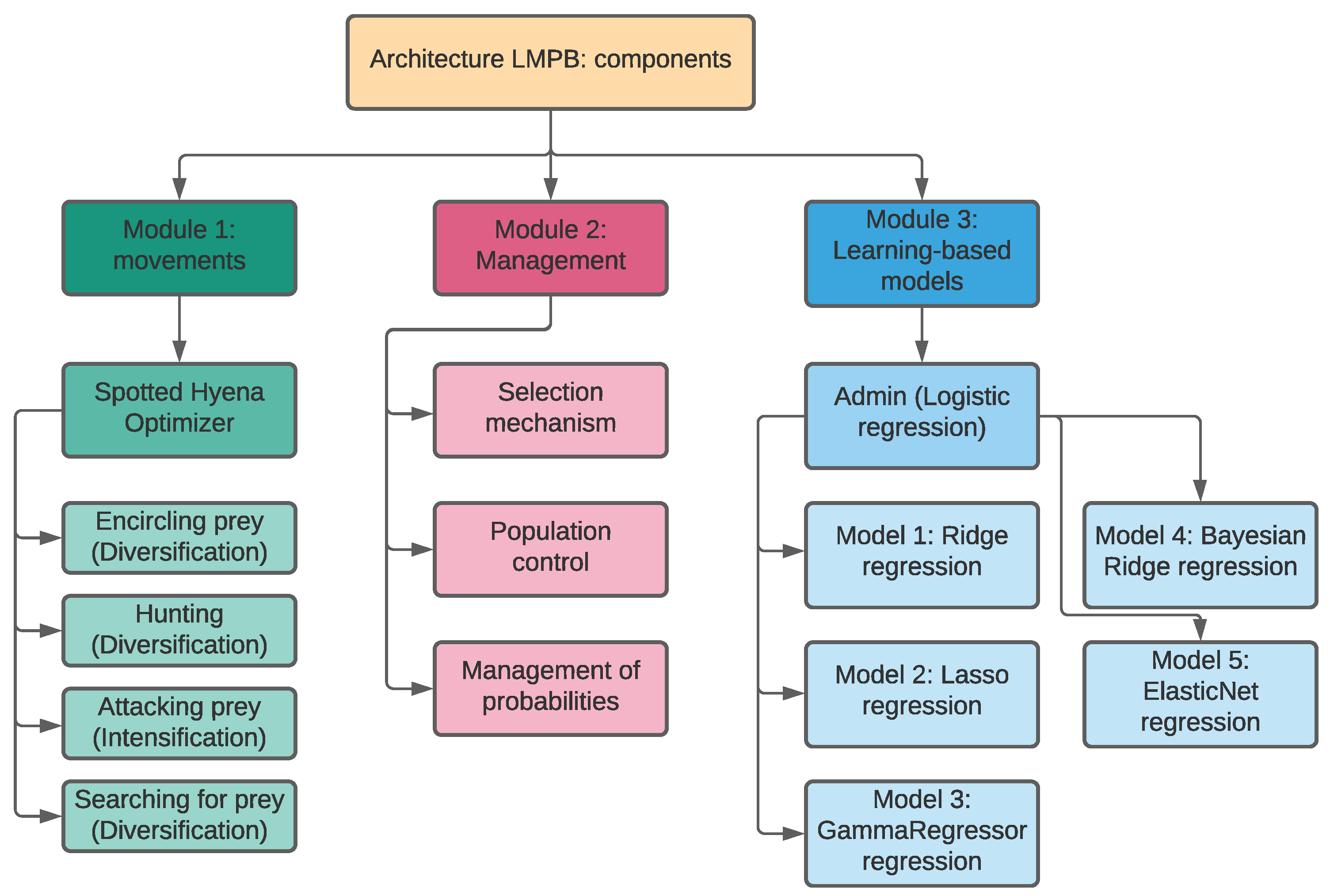
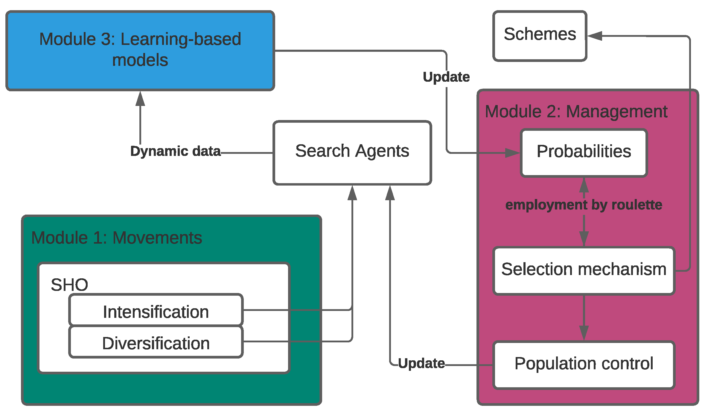
3.2. Proposed Modules
3.2.1. Module 1: Movements
3.2.2. Module 2: Management
3.2.3. Module 3: Learning-Based Methods
3.3. Proposed Algorithm
| Algorithm 1Proposed Architecture |
|
| Algorithm 2Learning Model |
|
4. Experimental Results
4.1. Continuous Optimization Problem
- if
- 0 if
- if
4.1.1. Algorithms Used and Results Comparison
4.1.2. Overall Discussion
- Exploitation analysis: unimodal functions are suitable for benchmarking this issue, the good results achieved can be interpreted that LMPB successfully performed in terms of exploiting optimum values.
- Exploration analysis: multimodal functions are suitable for benchmarking this issue, the competitive performance has proved its merits in terms of exploration and local minima avoidance.
4.2. Discrete Optimization Problem
4.2.1. Algorithms Used and Results Comparison
4.2.2. Overall Discussion
5. Conclusions and Future Work
Author Contributions
Funding
Institutional Review Board Statement
Informed Consent Statement
Data Availability Statement
Conflicts of Interest
References
- Yang, Y.; Zhang, Y.; Meng, X. A data-driven approach for optimizing the EV charging stations network. IEEE Access 2020, 8, 118572–118592. [Google Scholar] [CrossRef]
- Wu, Z.; Hu, J.; Ai, X.; Yang, G. Data-driven approaches for optimizing EV aggregator power profile in energy and reserve market. Int. J. Electr. Power Energy Syst. 2021, 129, 106808. [Google Scholar] [CrossRef]
- Wei, Y.; Zhang, X.; Shi, Y.; Xia, L.; Pan, S.; Wu, J.; Han, M.; Zhao, X. A review of data-driven approaches for prediction and classification of building energy consumption. Renew. Sustain. Energy Rev. 2018, 82, 1027–1047. [Google Scholar] [CrossRef]
- Khajehzadeh, M.; Taha, M.R.; El-Shafie, A.; Eslami, M. A survey on meta-heuristic global optimization algorithms. Res. J. Appl. Sci. Eng. Technol. 2011, 3, 569–578. [Google Scholar]
- Stork, J.; Eiben, A.E.; Bartz-Beielstein, T. A new taxonomy of global optimization algorithms. Nat. Comput. 2020, 21, 1–24. [Google Scholar] [CrossRef]
- Searle, S.R.; Gruber, M.H. Linear Models; John Wiley & Sons: Hoboken, NJ, USA, 2016. [Google Scholar]
- Hastie, T.J.; Pregibon, D. Generalized linear models. In Statistical Models in S; Routledge: London, UK, 2017; pp. 195–247. [Google Scholar]
- Pedregosa, F.; Varoquaux, G.; Gramfort, A.; Michel, V.; Thirion, B.; Grisel, O.; Blondel, M.; Prettenhofer, P.; Weiss, R.; Dubourg, V.; et al. Scikit-learn: Machine learning in Python. J. Mach. Learn. Res. 2011, 12, 2825–2830. [Google Scholar]
- Dhiman, G.; Kumar, V. Spotted hyena optimizer: A novel bio-inspired based metaheuristic technique for engineering applications. Adv. Eng. Softw. 2017, 114, 48–70. [Google Scholar] [CrossRef]
- Luo, Q.; Li, J.; Zhou, Y.; Liao, L. Using spotted hyena optimizer for training feedforward neural networks. Cogn. Syst. Res. 2021, 65, 1–16. [Google Scholar] [CrossRef]
- Vega, E.; Soto, R.; Crawford, B.; Peña, J.; Castro, C. A learning-based hybrid framework for dynamic balancing of exploration-exploitation: Combining regression analysis and metaheuristics. Mathematics 2021, 9, 1976. [Google Scholar] [CrossRef]
- Glover, F. Future paths for integer programming and links to artificial intelligence. Comput. Oper. Res. 1986, 13, 533–549. [Google Scholar] [CrossRef]
- Kirkpatrick, S. Optimization by simulated annealing: Quantitative studies. J. Stat. Phys. 1984, 34, 975–986. [Google Scholar] [CrossRef]
- Talbi, E.G. Combining metaheuristics with mathematical programming, constraint programming and machine learning. Ann. Oper. Res. 2016, 240, 171–215. [Google Scholar] [CrossRef]
- Song, H.; Triguero, I.; Özcan, E. A review on the self and dual interactions between machine learning and optimisation. Prog. Artif. Intell. 2019, 8, 143–165. [Google Scholar] [CrossRef]
- Talbi, E.G. Machine learning into metaheuristics: A survey and taxonomy. ACM Comput. Surv. 2021, 54, 1–32. [Google Scholar] [CrossRef]
- Jourdan, L.; Dhaenens, C.; Talbi, E.G. Using datamining techniques to help metaheuristics: A short survey. In International Workshop on Hybrid Metaheuristics; Springer: Berlin/Heidelberg, Germany, 2006; pp. 57–69. [Google Scholar]
- Jin, Y. A comprehensive survey of fitness approximation in evolutionary computation. Soft Comput. 2005, 9, 3–12. [Google Scholar] [CrossRef]
- Hong, T.P.; Wang, H.S.; Chen, W.C. Simultaneously applying multiple mutation operators in genetic algorithms. J. Heuristics 2000, 6, 439–455. [Google Scholar] [CrossRef]
- Ramsey, C.L.; Grefenstette, J.J. Case-Based Initialization of Genetic Algorithms. In Proceedings of the 5th International Conference on Genetic Algorithms, Urbana-Champaign, IL, USA, 1 June 1993; pp. 84–91. [Google Scholar]
- Dalboni, F.L.; Ochi, L.S.; Drummond, L.M.A. On improving evolutionary algorithms by using data mining for the oil collector vehicle routing problem. In Proceedings of the International Network Optimization Conference, Evry/Paris, France, 27–29 October 2003; pp. 182–188. [Google Scholar]
- Santos, H.G.; Ochi, L.S.; Marinho, E.H.; Drummond, L.M.D.A. Combining an evolutionary algorithm with data mining to solve a single-vehicle routing problem. Neurocomputing 2006, 70, 70–77. [Google Scholar] [CrossRef]
- Calvet, L.; de Armas, J.; Masip, D.; Juan, A.A. Learnheuristics: Hybridizing metaheuristics with machine learning for optimization with dynamic inputs. Open Math. 2017, 15, 261–280. [Google Scholar] [CrossRef]
- Jong, K.D. Parameter setting in EAs: A 30 year perspective. In Parameter Setting in Evolutionary Algorithms; Springer: Berlin/Heidelberg, Gemrany, 2007; pp. 1–18. [Google Scholar]
- Karimi-Mamaghan, M.; Mohammadi, M.; Meyer, P.; Karimi-Mamaghan, A.M.; Talbi, E.G. Machine Learning at the service of Meta-heuristics for solving Combinatorial Optimization Problems: A state-of-the-art. Eur. J. Oper. Res. 2022, 296, 393–422. [Google Scholar] [CrossRef]
- Talbi, E.G. Metaheuristics: From Design to Implementation; John Wiley & Sons: Hoboken, NJ, USA, 2009; Volume 74. [Google Scholar]
- Zennaki, M.; Ech-Cherif, A. A new machine learning based approach for tuning metaheuristics for the solution of hard combinatorial optimization problems. J. Appl. Sci. 2010, 10, 1991–2000. [Google Scholar] [CrossRef]
- Trindade, Á.R.; Campelo, F. Tuning metaheuristics by sequential optimisation of regression models. Appl. Soft Comput. 2019, 85, 105829. [Google Scholar] [CrossRef]
- Caserta, M.; Rico, E.Q. A cross entropy-Lagrangean hybrid algorithm for the multi-item capacitated lot-sizing problem with setup times. Comput. Oper. Res. 2009, 36, 530–548. [Google Scholar] [CrossRef]
- Soto, R.; Crawford, B.; Vega, E.; Gómez, A.; Gómez-Pulido, J.A. Solving the Set Covering Problem Using Spotted Hyena Optimizer and Autonomous Search. In Advances and Trends in Artificial Intelligence. From Theory to Practice; IEA/AIE 2019; Wotawa, F., Friedrich, G., Pill, I., Koitz-Hristov, R., Ali, M., Eds.; Lecture Notes in Computer Science; Springer: Cham, Switzerland, 2019; Volume 11606. [Google Scholar]
- Soto, R.; Crawford, B.; González, F.; Vega, E.; Castro, C.; Paredes, F. Solving the Manufacturing Cell Design Problem Using Human BehaviorBased Algorithm Supported by Autonomous Search. IEEE Access 2019, 7, 132228–132239. [Google Scholar] [CrossRef]
- Egwim, C.N.; Egunjobi, O.O.; Gomes, A.; Alaka, H. A Comparative Study on Machine Learning Algorithms for Assessing Energy Efficiency of Buildings. In Proceedings of the Joint European Conference on Machine Learning and Knowledge Discovery in Databases, Online, 13–17 September 2021; Springer: Cham, Switzerland, 2021; pp. 546–566. [Google Scholar]
- Menard, S. Applied Logistic Regression Analysis; Sage: Newcastle upon Tyne, UK, 2002; Volume 106. [Google Scholar]
- Tibshirani, R. Regression shrinkage and selection via the lasso. J. R. Stat. Soc. Ser. 1996, 58, 267–288. [Google Scholar] [CrossRef]
- McDonald, G.C. Ridge regression. Wiley Interdiscip. Rev. Comput. Stat. 2009, 1, 93–100. [Google Scholar] [CrossRef]
- Akwimbi, J. Modelling The Growth of Pension Funds Using Generalized Linear Model (gamma Regression). Ph.D. Thesis, University of Nairobi, Nairobi, Kenya, 2014. [Google Scholar]
- Yu, L.; Ma, X.; Wu, W.; Wang, Y.; Zeng, B. A novel elastic net-based NGBMC (1, n) model with multi-objective optimization for nonlinear time series forecasting. Commun. Nonlinear Sci. Numer. Simul. 2021, 96, 105696. [Google Scholar] [CrossRef]
- Gelman, A.; Carlin, J.B.; Stern, H.S.; Rubin, D.B. Bayesian Data Analysis; Chapman and Hall/CRC: Boca Raton, FL, USA, 1995. [Google Scholar]
- Digalakis, J.; Margaritis, K. On benchmarking functions for genetic algorithms. Int. J. Comput. Math 2001, 77, 481–506. [Google Scholar] [CrossRef]
- Yang, X. Firefly algorithm, stochastic test functions and design optimisation. Int. J. Bio-Inspired Comput. 2010, 2, 78–84. [Google Scholar] [CrossRef]
- Mirjalili, S.; Lewis, A. The Whale Optimization Algorithm. Adv. Eng. Softw. 2016, 95, 51–67. [Google Scholar] [CrossRef]
- Cortés-Toro, E.M.; Crawford, B.; Gómez-Pulido, J.A.; Soto, R.; Lanza-Gutiérrez, J.M. A New Metaheuristic Inspired by the Vapour-Liquid Equilibrium for Continuous Optimization. Appl. Sci. 2018, 8, 2080. [Google Scholar] [CrossRef]
- Mirjalili, S.; Mirjalili, S.M.; Lewis, A. Grey Wolf Optimizer. Adv. Eng. Softw. 2014, 69, 46–61. [Google Scholar] [CrossRef]
- Kennedy, J.; Eberhart, R. Particle swarm optimization. In Proceedings of the IEEE International Conference on Neural Networks, Perth, Australia, 27 November–1 December 1995; pp. 1942–1948. [Google Scholar]
- Rashedi, E.; Nezamabadi-Pour, H.; Saryazdi, S. GSA: A Gravitational Search Algorithm. Inf. Sci. 2009, 179, 2232–2248. [Google Scholar] [CrossRef]
- Storn, R.; Price, K. Differential Evolution—A Simple and Efficient Heuristic for global Optimization over Continuous Spaces. J. Glob. Optim. 1997, 11, 341–359. [Google Scholar] [CrossRef]
- Xu, J.; Yan, F. Hybrid Nelder–Mead algorithm and dragonfly algorithm for function optimization and the training of a multilayer perceptron. Arab. J. Sci. Eng. 2019, 44, 3473–3487. [Google Scholar] [CrossRef]
- Pisinger, D. The quadratic knapsack problem—A survey. Discrete applied mathematics. Discret. Appl. Math. 2007, 155, 623–648. [Google Scholar] [CrossRef]
- Horowitz, E.; Sahni, S. Computing partitions with applications to the knapsack problem. J. ACM 1974, 21, 277–292. [Google Scholar] [CrossRef]
- Mirjalili, S.; Lewis, A. S-shaped versus v-shaped transfer functions for binary particle swarm optimization. Swarm Evol. Comput. 2013, 9, 1–14. [Google Scholar] [CrossRef]
- Lanza-Gutierrez, J.M.; Crawford, B.; Soto, R.; Berrios, N.; Gomez-Pulido, J.A.; Paredes, F. Analyzing the effects of binarization techniques when solving the set covering problem through swarm optimization. Expert Syst. Appl. 2017, 70, 67–82. [Google Scholar] [CrossRef]
- Khemakhem, M.; Haddar, B.; Chebil, K.; Hanafi, S. A Filter-and-Fan Metaheuristic for the 0–1 Multidimensional Knapsack Problem. Int. J. Appl. Metaheuristic Comput. 2012, 3, 43–63. [Google Scholar] [CrossRef]
- Chih, M. Three pseudo-utility ratio-inspired particle swarm optimization with local search for multidimensional knapsack problem. Swarm Evol. Comput. 2018, 39, 279–296. [Google Scholar] [CrossRef]
- Haddar, B.; Khemakhem, M.; Hanafi, S.; Wilbaut, C. A hybrid quantum particle swarm optimization for the multidimensional knapsack problem. Eng. Appl. Artif. Intell. 2016, 55, 1–13. [Google Scholar] [CrossRef]
- Lemus-Romani, J.; Becerra-Rozas, M.; Crawford, B.; Soto, R.; Cisternas-Caneo, F.; Vega, E.; García, J. A novel learning-based binarization scheme selector for swarm algorithms solving combinatorial problems. Mathematics 2021, 9, 2887. [Google Scholar] [CrossRef]


| ID | Amount of Agents |
|---|---|
| scheme 1 | 20 |
| scheme 2 | 30 |
| scheme 3 | 40 |
| scheme 4 | 50 |
| ID | Probability to Be Selected |
|---|---|
| scheme 1 | 0.25 |
| scheme 2 | 0.25 |
| scheme 3 | 0.25 |
| scheme 4 | 0.25 |
| ID | Probability to Be Selected |
|---|---|
| scheme 1 | 0.20 |
| scheme 2 | 0.20 |
| scheme 3 | 0.40 |
| scheme 4 | 0.20 |
| Parameters | Values |
|---|---|
| Search agents | Scheme (20, 30, 40, 50) |
| Control parameter (h) | [5, 0] |
| M constant | [0.5, 1] |
| Number of generations | 5000 |
| 50 | |
| 1000 |
| Function | Search Subsets | Opt | Sol |
|---|---|---|---|
| (x) | 0 | ||
| (x) | 0 | ||
| (x) | 0 | ||
| (x) | 0 | ||
| (x) | −12596.487 | ||
| (x) | 0 | ||
| (x) | 0 | ||
| (x) | 0 | ||
| (x) | 0 | ||
| (x) | 1 | ||
| (x) | −1.0316285 | (0.08983, −0.7126) and (−0.08983, 0.7126) | |
| (x) | for and for | 0.397887 | (−3.142, 12.275), (3.142, 2.275), and (9.425, 2.425) |
| (x) | 3 | (0, −1) | |
| (x) | −3.86 | (0.114, 0.556, 0.852) | |
| (x) | −3.32 | (0.201, 0.150, 0.477, 0.275, 0.275, 0.377, 0.657) |
| i | |||||||
|---|---|---|---|---|---|---|---|
| 1 | 3 | 10 | 30 | 1 | 0.3689 | 0.1170 | 0.2673 |
| 2 | 0.1 | 10 | 35 | 1.2 | 0.4699 | 0.4387 | 0.7470 |
| 3 | 3 | 10 | 30 | 3 | 0.1091 | 0.8732 | 0.5547 |
| 4 | 0.1 | 10 | 30 | 3.2 | 0.03815 | 0.5743 | 0.8828 |
| i | |||||||||||||
|---|---|---|---|---|---|---|---|---|---|---|---|---|---|
| 1 | 10 | 3 | 17 | 3.5 | 1.7 | 8 | 1 | 0.131 | 0.169 | 0.556 | 0.012 | 0.828 | 0.588 |
| 2 | 0.05 | 10 | 17 | 0.1 | 8 | 14 | 1.2 | 0.232 | 0.413 | 0.830 | 0.373 | 0.100 | 0.999 |
| 3 | 3 | 3.5 | 1.7 | 10 | 17 | 8 | 3 | 0.234 | 0.141 | 0.352 | 0.288 | 0.304 | 0.665 |
| 4 | 17 | 8 | 0.05 | 10 | 0.1 | 14 | 3.2 | 0.404 | 0.882 | 0.873 | 0.574 | 0.109 | 0.038 |
| F | LMPB | WOA | DE | GSA | PSO | VLE | INMDA | |||||||
|---|---|---|---|---|---|---|---|---|---|---|---|---|---|---|
| Avg | StdDev | Avg | StdDev | Avg | StdDev | Avg | StdDev | Avg | StdDev | Avg | StdDev | Avg | StdDev | |
| 0.0907 | 2.0386 | 0.0000 | 0.0000 | 0.0000 | 0.0000 | 0.0000 | ||||||||
| 0.0346 | 0.5293 | 0.0000 | 0.0000 | 0.1941 | 0.0000 | 0.0000 | ||||||||
| 0.0000 | 0.0000 | 70.126 | 22.119 | 5.2020 | 0.7986 | 0.0000 | 0.0000 | |||||||
| 28.5342 | 70.0454 | 27.866 | 0.7636 | 0.0000 | 0.0000 | 67.543 | 62.225 | 96.718 | 60.116 | 79.199 | 37.400 | 0.0000 | 0.0000 | |
| F | LMPB | WOA | DE | GSA | PSO | VLE | INMDA | |||||||
|---|---|---|---|---|---|---|---|---|---|---|---|---|---|---|
| Avg | StdDev | Avg | StdDev | Avg | StdDev | Avg | StdDev | Avg | StdDev | Avg | StdDev | Avg | StdDev | |
| −914.1975 | 4974.5174 | 68.705 | −2245.1500 | 2.8400 | ||||||||||
| 0.1865 | 5.2889 | 0.0000 | 0.0000 | 69.200 | 38.800 | 25.968 | 7.4701 | 46.704 | 11.629 | 34.5830 | 17.8860 | 0.0000 | 0.0000 | |
| 7.6581 | 9.7217 | 7.4043 | 9.8976 | 0.23628 | 0.27602 | 0.50901 | 3.1704 | 3.9211 | 0.0000 | |||||
| 0.0056 | 0.1538 | 0.0000 | 0.0000 | 27.702 | 5.0403 | 0.5074 | 0.5041 | 0.0000 | 0.0000 | |||||
| 1.8286 | 0.3397 | 0.2149 | 1.7996 | 0.95114 | 0.2369 | 0.2877 | 0.0000 | 0.0000 | ||||||
| F | LMPB | WOA | DE | GSA | PSO | VLE | INMDA | |||||||
|---|---|---|---|---|---|---|---|---|---|---|---|---|---|---|
| Avg | StdDev | Avg | StdDev | Avg | StdDev | Avg | StdDev | Avg | StdDev | Avg | StdDev | Avg | StdDev | |
| 11.6858 | 7.8237 | 2.1120 | 2.4986 | 0.99800 | 5.8598 | 3.8313 | 3.6272 | 2.5608 | 0.99800 | N/A | N/A | |||
| 0.0001 | 0.0022 | −1.0316 | −1.0316 | −1.0316 | −1.0315 | N/A | N/A | |||||||
| −1.3549 | 0.2814 | 0.39791 | 0.39789 | 0.39789 | 0.0000 | 0.39789 | 0.0000 | 0.39815 | N/A | N/A | ||||
| 0.0001 | 0.0022 | 3.0000 | 3.0000 | 3.0000 | 3.0000 | 3.0097 | N/A | N/A | ||||||
| −1.4299 | 0.7508 | −3.8562 | N/A | N/A | −3.8628 | −3.8628 | −3.8628 | N/A | N/A | |||||
| −0.8621 | 0.4242 | −2.9811 | 0.37665 | N/A | N/A | −3.3178 | −3.2663 | −3.3179 | N/A | N/A | ||||
| F | Opt | LMPB | |||||||||
|---|---|---|---|---|---|---|---|---|---|---|---|
| Best | Worst | Avg | StdDev | Avg Time (s) | Best | Worst | Avg | StdDev | Avg Time (s) | ||
| 0 | 0 | 28.2786 | 0.0907 | 2.0386 | 150.1993 | 0 | 0 | 0 | 0 | 50.2377 | |
| 0 | 0 | 14.7092 | 0.0346 | 0.5293 | 190.9703 | 0 | 0 | 0 | 0 | 80.7524 | |
| 0 | 0 | 0 | 0 | 0 | 986.8423 | 0 | 0 | 0 | 0 | 96.3627 | |
| 0 | 0 | 29.4957 | 28.5342 | 70.0454 | 296.1747 | 71.0024 | |||||
| −12569.487 | −12569.487 | 9016.3258 | −914.1975 | 4974.5174 | 250.7817 | 0.0014 | 110.3354 | ||||
| 0 | 0 | 1.8934 | 0.1865 | 1.2189 | 217.4014 | 0 | 0 | 0 | 0 | 60.6482 | |
| 0 | 0 | 20.0001 | 7.6581 | 9.7217 | 427.1252 | 0 | 24.9122 | ||||
| 0 | 0 | 7.3880 | 0.0056 | 0.1538 | 255.7067 | 0 | 0 | 0 | 0 | 21.7758 | |
| 0 | 1.8290 | 1.8290 | 1.8290 | 0 | 2223.4575 | 1.8285 | 1.8286 | 1.8286 | 24.9172 | ||
| 1 | 6.9407 | 12.7187 | 11.6858 | 7.8237 | 901.5922 | 1 | 1 | 1 | 0 | 17.5661 | |
| −1.0316 | 0 | 0.0233 | 0.0001 | 0.0022 | 142.0010 | 0 | 0 | 0 | 0 | 7.5244 | |
| 0.3979 | −1.1395 | −1.5122 | −1.3549 | 0.2814 | 23.0392 | 1.1905 | 2.0325 | 1.5436 | 0.4223 | 4.5528 | |
| 3 | 0.0012 | 0 | 0.0001 | 0.0022 | 129.0010 | 32.6845 | 32.6845 | 32.6845 | 3.6846 | ||
| −3.86 | −2.0080 | −0.0554 | −1.4299 | 0.7508 | 229.6161 | −2.0081 | −2.0080 | −2.0081 | 7.1120 | ||
| −3.32 | −1.1676 | −0.0056 | −0.8621 | 0.4242 | 330.3406 | −2.1676 | −2.1676 | −2.1676 | 0 | 8.1145 | |
| F | Opt | LMPB | SHO-IRace | ||||||||
|---|---|---|---|---|---|---|---|---|---|---|---|
| Best | Worst | Avg | StdDev | Avg Time (s) | Best | Worst | Avg | StdDev | Avg Time (s) | ||
| 0 | 0 | 28.2786 | 0.0907 | 2.0386 | 150.1993 | 0 | 86.4729 | 0.1002 | 2.1974 | 130.2574 | |
| 0 | 0 | 14.7092 | 0.0346 | 0.5293 | 190.9703 | 0 | 22.2119 | 0.0362 | 0.5566 | 181.1410 | |
| 0 | 0 | 0 | 0 | 0 | 986.8423 | 0 | 2118.0295 | 97.4849 | 352.2949 | 882.2675 | |
| 0 | 0 | 29.4957 | 28.5342 | 70.0454 | 296.1747 | 0 | 188.6322 | 28.5221 | 69.3946 | 271.6308 | |
| −12569.487 | −12569.487 | 9016.3258 | −914.1975 | 4974.5174 | 250.7817 | −12569.4862 | 9016.3365 | −925.5051 | 4981.0787 | 229.1431 | |
| 0 | 0 | 1.8934 | 0.1865 | 1.2189 | 217.4014 | 0 | 2382.5545 | 0.2687 | 13.1434 | 163.7028 | |
| 0 | 0 | 20.0001 | 7.6581 | 9.7217 | 427.1252 | 22.2358 | 7.3976 | 9.6549 | 325.4619 | ||
| 0 | 0 | 7.3880 | 0.0056 | 0.1538 | 255.7067 | 0 | 3.4690 | 0.0593 | 0.4755 | 195.3925 | |
| 0 | 1.8290 | 1.8290 | 1.8290 | 0 | 2223.4575 | 35.5837 | 1766.7315 | 526.3003 | 410.1304 | 2060.7682 | |
| 1 | 6.9407 | 12.7187 | 11.6858 | 7.8237 | 901.5922 | 12.7186 | 498.9434 | 13.1147 | 9.6306 | 855.9498 | |
| −1.0316 | 0 | 0.0233 | 0.0001 | 0.0022 | 142.0010 | 0 | 0.1745 | 0.0001 | 0.0021 | 120.5488 | |
| 0.3979 | −1.1395 | −1.5122 | −1.3549 | 0.2814 | 23.0392 | −1.1395 | −1.6328 | −1.4191 | 0.2372 | 21.7540 | |
| 3 | 0.0012 | 0 | 0.0001 | 0.0022 | 129.0010 | 32.6846 | 635.1801 | 255.2925 | 237.1631 | 204.8439 | |
| −3.86 | −2.0080 | −0.0554 | −1.4299 | 0.7508 | 229.6161 | −2.0080 | 0.0467 | -1.2319 | 0.7848 | 183.3399 | |
| −3.32 | −1.1676 | −0.0056 | −0.8621 | 0.4242 | 330.3406 | −2.0080 | −1.6155 | −0.8480 | 0.4529 | 313.5484 | |
| ID | Test Problem | Optimal Solution | n | m |
|---|---|---|---|---|
| mknapcb1 | 5.100.00 | 24381 | 100 | 5 |
| 5.100.01 | 24274 | 100 | 5 | |
| 5.100.02 | 23551 | 100 | 5 | |
| 5.100.03 | 23534 | 100 | 5 | |
| 5.100.04 | 23991 | 100 | 5 | |
| mknapcb2 | 5.250.00 | 59312 | 250 | 5 |
| 5.250.01 | 61472 | 250 | 5 | |
| 5.250.02 | 62130 | 250 | 5 | |
| 5.250.03 | 59463 | 250 | 5 | |
| 5.250.04 | 58951 | 250 | 5 | |
| mknapcb3 | 5.500.00 | 120148 | 500 | 5 |
| 5.500.01 | 117879 | 500 | 5 | |
| 5.500.02 | 121131 | 500 | 5 | |
| 5.500.03 | 120804 | 500 | 5 | |
| 5.500.04 | 122319 | 500 | 5 | |
| mknapcb4 | 10.100.00 | 23064 | 100 | 10 |
| 10.100.01 | 22801 | 100 | 10 | |
| 10.100.02 | 22131 | 100 | 10 | |
| 10.100.03 | 22772 | 100 | 10 | |
| 10.100.04 | 22751 | 100 | 10 | |
| mknapcb5 | 10.250.00 | 59187 | 250 | 10 |
| 10.250.01 | 58781 | 250 | 10 | |
| 10.250.02 | 58097 | 250 | 10 | |
| 10.250.03 | 61000 | 250 | 10 | |
| 10.250.04 | 58092 | 250 | 10 | |
| mknapcb6 | 10.500.00 | 117821 | 500 | 10 |
| 10.500.01 | 119249 | 500 | 10 | |
| 10.500.02 | 119215 | 500 | 10 | |
| 10.500.03 | 118829 | 500 | 10 | |
| 10.500.04 | 116530 | 500 | 10 |
| LMPB | QPSO | 3R—PSO | F & F | |||||||||||
|---|---|---|---|---|---|---|---|---|---|---|---|---|---|---|
| ID | Test Problem | Opt | Best | Avg | RPD (%) | Best | Avg | RPD (%) | Best | Avg | RPD (%) | Best | Avg | RPD (%) |
| 5.100.00 | 24381 | 24381 | 18193.2647 | 0.00 | 24381 | 24381 | 0.00 | 24381 | 24381 | 0.00 | 24381 | N/A | 0.00 | |
| 5.100.01 | 24274 | 24274 | 17674.1159 | 0.00 | 24274 | 24274 | 0.00 | 24274 | 24274 | 0.00 | 24274 | N/A | 0.00 | |
| 5.100.02 | 23551 | 23551 | 17860.9433 | 0.00 | 23551 | 23551 | 0.00 | 23538 | 23538 | 0.06 | 23551 | N/A | 0.00 | |
| 5.100.03 | 23534 | 23534 | 19692.4754 | 0.00 | 23534 | 23534 | 0.00 | 23534 | 23508 | 0.00 | 23534 | N/A | 0.00 | |
| mknapcb1 | 5.100.04 | 23991 | 23991 | 17863.3812 | 0.00 | 23991 | 23991 | 0.00 | 23991 | 23961 | 0.00 | 23991 | N/A | 0.00 |
| 5.250.00 | 59312 | 59312 | 46587.9561 | 0.00 | 59312 | 59312 | 0.00 | N/A | N/A | N/A | 59312 | N/A | 0.00 | |
| 5.250.01 | 61472 | 61472 | 47299.2074 | 0.00 | 61472 | 61470 | 0.00 | N/A | N/A | N/A | 61468 | N/A | 0.01 | |
| 5.250.02 | 62130 | 62130 | 49261.7206 | 0.00 | 62130 | 62130 | 0.00 | N/A | N/A | N/A | 62130 | N/A | 0.00 | |
| 5.250.03 | 59463 | 59463 | 46365.1888 | 0.00 | 59427 | 59427 | 0.06 | N/A | N/A | N/A | 59436 | N/A | 0.05 | |
| mknapcb2 | 5.250.04 | 58951 | 58951 | 47005.2385 | 0.00 | 58951 | 58951 | 0.00 | N/A | N/A | N/A | 58951 | N/A | 0.00 |
| 5.500.00 | 120148 | 101980 | 88110.0778 | 15.12 | 120130 | 120105 | 0.01 | 120141 | 102101 | 0.01 | 120134 | N/A | 0.01 | |
| 5.500.01 | 117879 | 99901 | 90506.6091 | 15.25 | 117844 | 117834 | 0.03 | 117864 | 117825 | 0.01 | 117864 | N/A | 0.01 | |
| 5.500.02 | 121131 | 102559 | 91014.0520 | 15.33 | 121112 | 121092 | 0.02 | 121129 | 121103 | 0.00 | 121131 | N/A | 0.00 | |
| 5.500.03 | 120804 | 100864 | 91796.0122 | 16.50 | 120804 | 120740 | 0.00 | 120804 | 120722 | 0.00 | 120794 | N/A | 0.01 | |
| mknapcb3 | 5.500.04 | 122319 | 102520 | 91771.7789 | 16.18 | 122319 | 122300 | 0.00 | 122319 | 122310 | 0.00 | 122319 | N/A | 0.00 |
| 10.100.00 | 23064 | 23064 | 22275.5321 | 0.00 | 23064 | 23064 | 0.00 | 23064 | 23050 | 0.00 | 23064 | N/A | 0.00 | |
| 10.100.01 | 22801 | 22801 | 21295.6074 | 0.00 | 22801 | 22801 | 0.00 | 22801 | 22752 | 0.00 | 22801 | N/A | 0.00 | |
| 10.100.02 | 22131 | 22131 | 20486.6556 | 0.00 | 22131 | 22131 | 0.00 | 22131 | 22119 | 0.00 | 22131 | N/A | 0.00 | |
| 10.100.03 | 22772 | 22772 | 18785.5884 | 0.00 | 22772 | 22772 | 0.00 | 22772 | 22744 | 0.00 | 22772 | N/A | 0.00 | |
| mknapcb4 | 10.100.04 | 22751 | 22751 | 22604.2587 | 0.00 | 22751 | 22751 | 0.00 | 22751 | 22651 | 0.00 | 22751 | N/A | 0.00 |
| 10.250.00 | 59187 | 59187 | 55818.9961 | 0.00 | 59182 | 59173 | 0.01 | N/A | N/A | N/A | 59164 | N/A | 0.04 | |
| 10.250.01 | 58781 | 58781 | 55302.6930 | 0.00 | 58781 | 58733 | 0.00 | N/A | N/A | N/A | 58693 | N/A | 0.15 | |
| 10.250.02 | 58097 | 58097 | 52907.7982 | 0.00 | 58097 | 58096 | 0.00 | N/A | N/A | N/A | 58094 | N/A | 0.01 | |
| 10.250.03 | 61000 | 61000 | 57342.3073 | 0.00 | 61000 | 60986 | 0.00 | N/A | N/A | N/A | 60972 | N/A | 0.05 | |
| mknapcb5 | 10.250.04 | 58092 | 58092 | 55037.2680 | 0.00 | 58092 | 58092 | 0.00 | N/A | N/A | N/A | 58092 | N/A | 0.00 |
| 10.500.00 | 117821 | 103226 | 93309.3655 | 12.38 | 117744 | 117733 | 0.07 | 117790 | 117699 | 0.03 | 117734 | N/A | 0.07 | |
| 10.500.01 | 119249 | 105088 | 96823.8780 | 11.87 | 119177 | 119148 | 0.06 | 119155 | 119125 | 0.08 | 119181 | N/A | 0.06 | |
| 10.500.02 | 119215 | 104870 | 96151.9076 | 12.03 | 119215 | 119146 | 0.00 | 119211 | 119094 | 0.00 | 119194 | N/A | 0.02 | |
| 10.500.03 | 118829 | 104308 | 95338.5665 | 12.22 | 118775 | 118747 | 0.05 | 118813 | 118754 | 0.01 | 118784 | N/A | 0.04 | |
| mknapcb6 | 10.500.04 | 116530 | 101380 | 92260.2844 | 13.00 | 116502 | 116449 | 0.02 | 116470 | 116509 | 0.05 | 116471 | N/A | 0.05 |
| LMPB | SHO-IRace | ||||||||||||
|---|---|---|---|---|---|---|---|---|---|---|---|---|---|
| ID | Opt | Best | Worst | Avg | StdDev | RPD (%) | Avg Time (s) | Best | Worst | Avg | StdDev | RPD (%) | Avg Time (s) |
| 5.100.00 | 24381 | 24381 | 17595 | 18193.2647 | 689.3522 | 0.00 | 4669.6999 | 20661 | 17595 | 18269.0889 | 719.6834 | 15.25 | 5872.1652 |
| 5.100.01 | 24274 | 24274 | 17401 | 17674.1159 | 522.1186 | 0.00 | 5697.6984 | 19792 | 17401 | 17680.8992 | 536.9595 | 18.46 | 5553.4974 |
| 5.100.02 | 23551 | 23551 | 17692 | 17860.9433 | 395.5785 | 0.00 | 4292.5007 | 20119 | 17692 | 17956.3902 | 485.5376 | 14.57 | 4467.5135 |
| 5.100.03 | 23534 | 23534 | 19685 | 19692.4754 | 49.3286 | 0.00 | 5347.2370 | 20703 | 19685 | 19692.8931 | 74.2092 | 12.02 | 3854.0709 |
| 5.100.04 | 23991 | 23991 | 17744 | 17863.3812 | 320.1172 | 0.00 | 5747.0107 | 19525 | 17744 | 17840.1698 | 265.9275 | 18.61 | 4897.6560 |
| 5.250.00 | 59312 | 59312 | 46049 | 46587.9561 | 858.5338 | 0.00 | 8670.5223 | 50256 | 46049 | 46612.2596 | 903.5159 | 15.26 | 6656.1823 |
| 5.250.01 | 61472 | 61472 | 46890 | 47299.2074 | 749.7909 | 0.00 | 7810.9763 | 51527 | 46890 | 47277.6690 | 738.8178 | 16.17 | 6568.5947 |
| 5.250.02 | 62130 | 62130 | 49237 | 49261.7206 | 163.3191 | 0.00 | 5671.1701 | 50292 | 49237 | 49257.9839 | 117.6427 | 19.05 | 4843.4766 |
| 5.250.03 | 59463 | 59463 | 42804 | 46365.1888 | 2137.5436 | 0.00 | 16606.7606 | 50890 | 42804 | 46275.6829 | 2190.8037 | 14.41 | 15333.6760 |
| 5.250.04 | 58951 | 58951 | 46870 | 47005.2385 | 369.0429 | 0.00 | 6987.2142 | 49893 | 46870 | 46979.8645 | 348.9194 | 15.36 | 6414.6560 |
| 5.500.00 | 120148 | 101980 | 73168 | 88110.0778 | 11544.9826 | 15.12 | 31594.7054 | 101400 | 73168 | 89634.3614 | 10969.3236 | 15.60 | 40985.2208 |
| 5.500.01 | 117879 | 99901 | 71265 | 90506.6091 | 11400.2546 | 15.25 | 41155.1138 | 99123 | 71265 | 90470.8571 | 11432.0737 | 15.91 | 41596.6308 |
| 5.500.02 | 121131 | 102559 | 74678 | 91014.0520 | 12735.6287 | 15.33 | 33245.1504 | 103579 | 74678 | 94113.1442 | 11512.8562 | 14.49 | 39693.0396 |
| 5.500.03 | 120804 | 100864 | 74715 | 91769.0122 | 10609.5044 | 16.50 | 44675.9107 | 101572 | 74715 | 91395.0128 | 10851.0576 | 15.92 | 39272.9026 |
| 5.500.04 | 122319 | 102520 | 74537 | 91771.7789 | 10591.1422 | 16.18 | 42645.1608 | 102057 | 74537 | 90647.5024 | 11272.3193 | 16.56 | 43738.2077 |
| 10.100.00 | 23064 | 23064 | 17298 | 22275.5321 | 670.6074 | 0.00 | 7179.9602 | 19751 | 17298 | 17766.0012 | 587.7123 | 14.36 | 8278.5790 |
| 10.100.01 | 22801 | 22801 | 17352 | 21295.5074 | 44.2336 | 0.00 | 6618.0995 | 19081 | 17352 | 17470.8750 | 284.2832 | 16.31 | 4660.8592 |
| 10.100.02 | 22131 | 22131 | 15699 | 20486.6556 | 948.5033 | 0.00 | 8081.3328 | 19342 | 15699 | 16531.9192 | 901.2227 | 12.60 | 5975.8820 |
| 10.100.03 | 22772 | 22772 | 18817 | 19795.5884 | 469.0794 | 0.00 | 6866.3064 | 20017 | 18817 | 18861.1892 | 148.7656 | 12.09 | 5070.9132 |
| 10.100.04 | 22751 | 22751 | 17564 | 22604.2587 | 436.9923 | 0.00 | 6945.8575 | 19667 | 17564 | 17804.0787 | 443.9254 | 13.55 | 5626.2527 |
| 10.250.00 | 59187 | 59187 | 48086 | 55818.9961 | 11675.8756 | 0.00 | 9550.5818 | 52250 | 48086 | 48545.8764 | 815.5280 | 11.72 | 7242.5197 |
| 10.250.01 | 58781 | 58781 | 43173 | 55302.6930 | 5750.7501 | 0.00 | 13587.1938 | 50869 | 43173 | 46824.4194 | 3789.4850 | 13.46 | 8701.9378 |
| 10.250.02 | 58097 | 58097 | 45538 | 52907.7982 | 10827.5062 | 0.00 | 15849.1611 | 50261 | 45538 | 46420.7704 | 1018.7772 | 13.48 | 13069.1670 |
| 10.250.03 | 61000 | 61000 | 47587 | 57342.3073 | 10802.1653 | 0.00 | 11107.4894 | 52286 | 47587 | 48855.7066 | 1996.1527 | 14.28 | 6072.3390 |
| 10.250.04 | 58092 | 58092 | 47703 | 55037.2680 | 11251.2648 | 0.00 | 9075.8829 | 51403 | 47703 | 48273.0614 | 868.3146 | 11.51 | 7042.7040 |
| 10.500.00 | 117821 | 103226 | 74746 | 93309.3655 | 13265.1931 | 12.38 | 33763.7203 | 103608 | 74746 | 91656.5522 | 13723.0371 | 12.06 | 30478.6163 |
| 10.500.01 | 119249 | 105088 | 76531 | 96823.8780 | 12237.0902 | 11.87 | 38343.9976 | 104996 | 76531 | 97534.9325 | 11834.3923 | 11.95 | 42585.3414 |
| 10.500.02 | 119215 | 104870 | 74620 | 96151.9076 | 11857.6879 | 12.03 | 46075.8874 | 105329 | 74620 | 95092.7730 | 12464.6680 | 11.64 | 37875.6117 |
| 10.500.03 | 118829 | 104308 | 74845 | 95338.5665 | 11119.6133 | 12.22 | 47983.9497 | 103663 | 74845 | 94803.7957 | 11431.0257 | 12.76 | 43169.6069 |
| 10.500.04 | 116530 | 101380 | 74441 | 92260.2844 | 10578.1152 | 13.00 | 43098.1306 | 101869 | 74441 | 92366.4123 | 10647.4900 | 12.58 | 43326.2896 |
| LMPB | SHO | ||||||||||||
|---|---|---|---|---|---|---|---|---|---|---|---|---|---|
| ID | Opt | Best | Worst | Avg | StdDev | RPD (%) | Avg Time (s) | Best | Worst | Avg | StdDev | RPD (%) | Avg Time (s) |
| 5.100.00 | 24381 | 24381 | 17595 | 18193.2647 | 689.3522 | 0.00 | 4669.6999 | 17950 | 16391 | 17109.1000 | 658.0524 | 26.36 | 210.4372 |
| 5.100.01 | 24274 | 24274 | 17401 | 17674.1159 | 522.1186 | 0.00 | 5697.6984 | 17854 | 16486 | 17055.0500 | 541.3379 | 26.44 | 181.5390 |
| 5.100.02 | 23551 | 23551 | 17692 | 17860.9433 | 395.5785 | 0.00 | 4292.5007 | 17886 | 16256 | 17297.0000 | 639.4370 | 24.05 | 150.7572 |
| 5.100.03 | 23534 | 23534 | 19685 | 19692.4754 | 49.3286 | 0.00 | 5347.2370 | 18445 | 17889 | 17963.2500 | 161.9119 | 21.62 | 190.4938 |
| 5.100.04 | 23991 | 23991 | 17744 | 17863.3812 | 320.1172 | 0.00 | 5747.0107 | 17678 | 17430 | 17528.4000 | 105.7115 | 26.31 | 140.3210 |
| 5.250.00 | 59312 | 59312 | 46049 | 46587.9561 | 858.5338 | 0.00 | 8670.5223 | 44891 | 44453 | 44596.0000 | 143.7212 | 24.31 | 1230.0471 |
| 5.250.01 | 61472 | 61472 | 46890 | 47299.2074 | 749.7909 | 0.00 | 7810.9763 | 45928 | 44306 | 45047.0000 | 480.1600 | 25.28 | 848.3955 |
| 5.250.02 | 62130 | 62130 | 49237 | 49261.7206 | 163.3191 | 0.00 | 5671.1701 | 42563 | 42520 | 42522.1500 | 9.3716 | 31.49 | 1292.4814 |
| 5.250.03 | 59463 | 59463 | 42804 | 46365.1888 | 2137.5436 | 0.00 | 16606.7606 | 46782 | 46038 | 46257.8500 | 272.5830 | 21.32 | 15333.6760 |
| 5.250.04 | 58951 | 58951 | 46870 | 47005.2385 | 369.0429 | 0.00 | 6987.2142 | 45445 | 43815 | 44565.4000 | 446.6804 | 22.91 | 1076.0837 |
| 5.500.00 | 120148 | 101980 | 73168 | 88110.0778 | 11544.9826 | 15.12 | 31594.7054 | 91110 | 89807 | 90131.7000 | 417.4011 | 24.16 | 2191.6924 |
| 5.500.01 | 117879 | 99901 | 71265 | 90506.6091 | 11400.2546 | 15.25 | 41155.1138 | 91701 | 89479 | 90880.9500 | 521.3980 | 22.20 | 2157.1687 |
| 5.500.02 | 121131 | 102559 | 74678 | 91014.0520 | 12735.6287 | 15.33 | 33245.1504 | 92436 | 91702 | 91753.8500 | 169.8229 | 23.68 | 2873.9049 |
| 5.500.03 | 120804 | 100864 | 74715 | 91769.0122 | 10609.5044 | 16.50 | 44675.9107 | 93638 | 91512 | 93040.6500 | 487.9807 | 22.48 | 2986.8021 |
| 5.500.04 | 122319 | 102520 | 74537 | 91771.7789 | 10591.1422 | 16.18 | 42645.1608 | 90328 | 87825 | 90077.7000 | 750.9000 | 26.15 | 2664.4909 |
| 10.100.00 | 23064 | 23064 | 17298 | 22275.5321 | 670.6074 | 0.00 | 7179.9602 | 19626 | 18043 | 19071.1000 | 576.5332 | 14.90 | 112.5756 |
| 10.100.01 | 22801 | 22801 | 17352 | 21295.5074 | 44.2336 | 0.00 | 6618.0995 | 17546 | 16036 | 17085.5500 | 377.4207 | 23.04 | 99.3756 |
| 10.100.02 | 22131 | 22131 | 15699 | 20486.6556 | 948.5033 | 0.00 | 8081.3328 | 18057 | 17012 | 17309.7000 | 337.4800 | 18.40 | 120.5140 |
| 10.100.03 | 22772 | 22772 | 18817 | 19795.5884 | 469.0794 | 0.00 | 6866.3064 | 20024 | 18755 | 19178.6000 | 401.2019 | 12.06 | 99.6616 |
| 10.100.04 | 22751 | 22751 | 17564 | 22604.2587 | 436.9923 | 0.00 | 6945.8575 | 18651 | 18099 | 18185.0000 | 171.6164 | 18.02 | 97.3623 |
| 10.250.00 | 59187 | 59187 | 48086 | 55818.9961 | 11675.8756 | 0.00 | 9550.5818 | 45143 | 44493 | 44914.5000 | 310.0302 | 23.72 | 566.9247 |
| 10.250.01 | 58781 | 58781 | 43173 | 55302.6930 | 5750.7501 | 0.00 | 13587.1938 | 48090 | 47356 | 47735.0500 | 297.7889 | 18.18 | 590.0571 |
| 10.250.02 | 58097 | 58097 | 45538 | 52907.7982 | 10827.5062 | 0.00 | 15849.1611 | 47536 | 45938 | 47088.3000 | 421.6500 | 18.17 | 492.0703 |
| 10.250.03 | 61000 | 61000 | 47587 | 57342.3073 | 10802.1653 | 0.00 | 11107.4894 | 47968 | 46884 | 47176.6500 | 330.7825 | 21.36 | 589.1354 |
| 10.250.04 | 58092 | 58092 | 47703 | 55037.2680 | 11251.2648 | 0.00 | 9075.8829 | 47139 | 44895 | 46559.7500 | 854.3255 | 18.85 | 933.7649 |
| 10.500.00 | 117821 | 103226 | 74746 | 93309.3655 | 13265.1931 | 12.38 | 33763.7203 | 90995 | 89690 | 90281.8000 | 381.1162 | 22.76 | 2665.9732 |
| 10.500.01 | 119249 | 105088 | 76531 | 96823.8780 | 12237.0902 | 11.87 | 38343.9976 | 90207 | 87691 | 89507.1500 | 602.0926 | 24.35 | 3015.1351 |
| 10.500.02 | 119215 | 104870 | 74620 | 96151.9076 | 11857.6879 | 12.03 | 46075.8874 | 94196 | 91359 | 92369.0500 | 615.9669 | 20.98 | 2569.8929 |
| 10.500.03 | 118829 | 104308 | 74845 | 95338.5665 | 11119.6133 | 12.22 | 47983.9497 | 94549 | 91796 | 93328.1000 | 614.4442 | 20.44 | 2707.8142 |
| 10.500.04 | 116530 | 101380 | 74441 | 92260.2844 | 10578.1152 | 13.00 | 43098.1306 | 91234 | 89336 | 90872.6500 | 450.8905 | 21.70 | 2465.6711 |
| LMPB | TS | ||||||||||||
|---|---|---|---|---|---|---|---|---|---|---|---|---|---|
| ID | Opt | Best | Worst | Avg | StdDev | RPD (%) | Avg Time (s) | Best | Worst | Avg | StdDev | RPD (%) | Avg Time (s) |
| 5.100.00 | 24381 | 24381 | 17595 | 18193.2647 | 689.3522 | 0.00 | 4669.6999 | 17920 | 14646 | 17200.2660 | 441.6150 | 26.50 | 9.2408 |
| 5.100.01 | 24274 | 24274 | 17401 | 17674.1159 | 522.1185 | 0.00 | 5697.6984 | 17895 | 15281 | 17209.6480 | 764.0746 | 26.28 | 8.1997 |
| 5.100.02 | 23551 | 23551 | 17692 | 17860.9432 | 395.5784 | 0.00 | 4292.5006 | 17557 | 15473 | 16471.3200 | 537.5266 | 25.45 | 9.0440 |
| 5.100.03 | 23534 | 23534 | 19685 | 19692.4753 | 49.3286 | 0.00 | 5347.2370 | 18153 | 14953 | 18068.7160 | 764.7306 | 22.86 | 6.9277 |
| 5.100.04 | 23991 | 23991 | 17744 | 17863.3811 | 320.1171 | 0.00 | 5747.0107 | 17599 | 15722 | 17760.1780 | 245.7550 | 26.64 | 8.1933 |
| 5.250.00 | 59312 | 59312 | 46049 | 46587.9560 | 858.5338 | 0.00 | 8670.5223 | 45431 | 41916 | 45392.1620 | 297.6204 | 23.40 | 51.9413 |
| 5.250.01 | 61472 | 61472 | 46890 | 47299.2073 | 749.7908 | 0.00 | 7810.9763 | 44651 | 39048 | 42666.3920 | 1629.9833 | 27.36 | 90.8240 |
| 5.250.02 | 62130 | 62130 | 49237 | 49261.7205 | 163.3190 | 0.00 | 5671.1700 | 44587 | 42244 | 43400.5440 | 710.5724 | 28.24 | 55.6142 |
| 5.250.03 | 59463 | 59463 | 42804 | 46365.1887 | 2137.5435 | 0.00 | 16606.7606 | 46510 | 40376 | 46108.0680 | 1191.6083 | 21.78 | 73.4146 |
| 5.250.04 | 58951 | 58951 | 46870 | 47005.2385 | 369.0429 | 0.00 | 6987.2141 | 43622 | 41511 | 43578.5660 | 235.7575 | 26.00 | 83.7176 |
| 5.500.00 | 120148 | 101980 | 73168 | 88110.0777 | 11544.9826 | 15.12 | 31594.7054 | 89365 | 85199 | 88040.6580 | 1055.1352 | 25.62 | 657.7096 |
| 5.500.01 | 117879 | 99901 | 71265 | 90506.6090 | 11400.2546 | 15.25 | 41155.1138 | 91192 | 87326 | 90738.1740 | 1051.4631 | 22.64 | 380.6708 |
| 5.500.02 | 121131 | 102559 | 74678 | 91014.0520 | 12735.6287 | 15.33 | 33245.1504 | 92155 | 87168 | 90280.1500 | 2329.0822 | 23.92 | 448.3687 |
| 5.500.03 | 120804 | 100864 | 74715 | 91769.0122 | 10609.5044 | 16.50 | 44675.9107 | 92344 | 88444 | 91129.6820 | 993.0370 | 23.56 | 417.6390 |
| 5.500.04 | 122319 | 102520 | 74537 | 91771.7788 | 10591.1422 | 16.18 | 42645.1608 | 86955 | 80832 | 85634.6120 | 985.2763 | 28.91 | 326.0826 |
| 10.100.00 | 23064 | 23064 | 17298 | 32275.5320 | 24670.6074 | 0.00 | 7179.9601 | 19365 | 17117 | 19292.6880 | 607.9159 | 16.04 | 4.2649 |
| 10.100.01 | 22801 | 22801 | 17352 | 31295.5074 | 24044.2336 | 0.00 | 6618.0994 | 18535 | 16420 | 17955.4980 | 714.6238 | 18.71 | 5.3840 |
| 10.100.02 | 22131 | 22131 | 15699 | 30486.6555 | 23948.5033 | 0.00 | 8081.3327 | 17523 | 14835 | 16785.3360 | 484.2500 | 20.82 | 3.3187 |
| 10.100.03 | 22772 | 22772 | 18817 | 32795.5884 | 24469.0794 | 0.00 | 6866.3063 | 18229 | 18179 | 18190.5000 | 21.0416 | 19.95 | 4.3792 |
| 10.100.04 | 22751 | 22751 | 17564 | 32604.2586 | 24436.9923 | 0.00 | 6945.8575 | 18833 | 17619 | 18463.4220 | 277.1007 | 17.22 | 4.9251 |
| 10.250.00 | 59187 | 59187 | 48086 | 55818.9960 | 11675.8756 | 0.00 | 9550.5818 | 44135 | 40025 | 43711.1320 | 933.0496 | 25.43 | 39.0509 |
| 10.250.01 | 58781 | 58781 | 43173 | 55302.6930 | 10750.7501 | 0.00 | 13587.1938 | 46438 | 42427 | 45226.7400 | 943.0535 | 21.00 | 47.0854 |
| 10.250.02 | 58097 | 58097 | 45538 | 52907.7982 | 10827.5062 | 0.00 | 15849.1611 | 44080 | 41890 | 43428.4520 | 463.4027 | 24.13 | 40.9750 |
| 10.250.03 | 61000 | 61000 | 47587 | 57342.3073 | 10802.1653 | 0.00 | 11107.4894 | 46377 | 45074 | 46255.3360 | 258.9354 | 23.97 | 43.8730 |
| 10.250.04 | 58092 | 58092 | 47703 | 55037.2679 | 11251.2648 | 0.00 | 9075.8829 | 43049 | 38232 | 42366.8760 | 981.8458 | 25.90 | 42.2721 |
| 10.500.00 | 117821 | 103226 | 74746 | 93309.3654 | 13265.1931 | 12.38 | 33763.7203 | 90919 | 89123 | 90331.2340 | 447.7161 | 22.83 | 178.1260 |
| 10.500.01 | 119249 | 105088 | 76531 | 96823.8780 | 12237.0902 | 11.87 | 38343.9976 | 91968 | 85869 | 91923.8820 | 1797.3181 | 22.88 | 231.8760 |
| 10.500.02 | 119215 | 104870 | 74620 | 96151.9075 | 11857.6879 | 12.03 | 46075.8874 | 95984 | 92567 | 95468.6580 | 1811.0270 | 19.49 | 270.4680 |
| 10.500.03 | 118829 | 104308 | 74845 | 95338.5664 | 11119.6133 | 12.22 | 47983.9497 | 91297 | 85080 | 90911.8560 | 1131.8605 | 23.17 | 197.9920 |
| 10.500.04 | 116530 | 101380 | 74441 | 92260.2844 | 10578.1152 | 13.00 | 43098.1306 | 92792 | 88027 | 93015.9780 | 1423.4816 | 20.37 | 342.9408 |
| LMPB | SA | ||||||||||||
|---|---|---|---|---|---|---|---|---|---|---|---|---|---|
| ID | Opt | Best | Worst | Avg | StdDev | RPD (%) | Avg Time (s) | Best | Worst | Avg | StdDev | RPD (%) | Avg Time (s) |
| 5.100.00 | 24381 | 24381 | 17595 | 18193.2647 | 689.3522 | 0.00 | 4669.6999 | 16645 | 15750 | 16488.2857 | 257.5163 | 31.73 | 15.5006 |
| 5.100.01 | 24274 | 24274 | 17401 | 17674.1159 | 522.1185 | 0.00 | 5697.6984 | 16732 | 15574 | 16061.4381 | 560.7617 | 31.07 | 15.0110 |
| 5.100.02 | 23551 | 23551 | 17692 | 17860.9432 | 395.5784 | 0.00 | 4292.5006 | 14663 | 13380 | 14398.9333 | 378.2078 | 37.74 | 9.1421 |
| 5.100.03 | 23534 | 23534 | 19685 | 19692.4753 | 49.3286 | 0.00 | 5347.2370 | 17033 | 14747 | 16594.0540 | 730.5726 | 27.62 | 10.4877 |
| 5.100.04 | 23991 | 23991 | 17744 | 17863.3811 | 320.1171 | 0.00 | 5747.0107 | 17106 | 16307 | 16974.1016 | 296.6305 | 28.70 | 12.3591 |
| 5.250.00 | 59312 | 59312 | 46049 | 46587.9560 | 858.5338 | 0.00 | 8670.5223 | 44861 | 43230 | 44563.9048 | 518.9806 | 24.36 | 76.2560 |
| 5.250.01 | 61472 | 61472 | 46890 | 47299.2073 | 749.7908 | 0.00 | 7810.9763 | 41902 | 41321 | 41646.1333 | 249.8855 | 31.84 | 65.4760 |
| 5.250.02 | 62130 | 62130 | 49237 | 49261.7205 | 163.3190 | 0.00 | 5671.1700 | 43316 | 40636 | 42807.8381 | 791.1798 | 30.28 | 54.3458 |
| 5.250.03 | 59463 | 59463 | 42804 | 46365.1887 | 2137.5435 | 0.00 | 16606.7606 | 48112 | 41941 | 46223.6159 | 2115.7624 | 19.09 | 72.0230 |
| 5.250.04 | 58951 | 58951 | 46870 | 47005.2385 | 369.0429 | 0.00 | 6987.2141 | 44235 | 42284 | 44005.2921 | 447.8486 | 24.96 | 91.7240 |
| 5.500.00 | 120148 | 101980 | 73168 | 88110.0777 | 11544.9826 | 15.12 | 31594.7054 | 91226 | 87931 | 90928.0222 | 669.9465 | 24.07 | 333.4513 |
| 5.500.01 | 117879 | 99901 | 71265 | 90506.6090 | 11400.2546 | 15.25 | 41155.1138 | 90749 | 88213 | 90514.8825 | 512.7554 | 23.02 | 365.0060 |
| 5.500.02 | 121131 | 102559 | 74678 | 91014.0520 | 12735.6287 | 15.33 | 33245.1504 | 88397 | 86003 | 87795.4984 | 701.4480 | 27.02 | 219.4263 |
| 5.500.03 | 120804 | 100864 | 74715 | 91769.0122 | 10609.5044 | 16.50 | 44675.9107 | 89615 | 88855 | 89479.8889 | 290.5674 | 25.82 | 289.9401 |
| 5.500.04 | 122319 | 102520 | 74537 | 91771.7788 | 10591.1422 | 16.18 | 42645.1608 | 87974 | 84700 | 87449.4000 | 952.0907 | 28.08 | 393.7943 |
| 10.100.00 | 23064 | 23064 | 17298 | 32275.5320 | 24670.6074 | 0.00 | 7179.9601 | 18645 | 17245 | 18052.5873 | 629.0033 | 19.16 | 7.8250 |
| 10.100.01 | 22801 | 22801 | 17352 | 31295.5074 | 24044.2336 | 0.00 | 6618.0994 | 18841 | 17515 | 18615.5016 | 423.9138 | 17.37 | 10.6280 |
| 10.100.02 | 22131 | 22131 | 15699 | 30486.6555 | 23948.5033 | 0.00 | 8081.3327 | 17465 | 16575 | 17456.6349 | 70.7870 | 21.08 | 8.9347 |
| 10.100.03 | 22772 | 22772 | 18817 | 32795.5884 | 24469.0794 | 0.00 | 6866.3063 | 18152 | 15786 | 17972.5873 | 402.4176 | 20.29 | 8.8359 |
| 10.100.04 | 22751 | 22751 | 17564 | 32604.2586 | 24436.9923 | 0.00 | 6945.8575 | 18705 | 17431 | 18372.9206 | 553.1250 | 17.78 | 8.9342 |
| 10.250.00 | 59187 | 59187 | 48086 | 55818.9960 | 11675.8756 | 0.00 | 9550.5818 | 43280 | 39946 | 42544.8889 | 940.8290 | 26.88 | 31.3592 |
| 10.250.01 | 58781 | 58781 | 43173 | 55302.6930 | 10750.7501 | 0.00 | 13587.1938 | 46785 | 43999 | 46371.5143 | 752.3758 | 20.41 | 56.4902 |
| 10.250.02 | 58097 | 58097 | 45538 | 52907.7982 | 10827.5062 | 0.00 | 15849.1611 | 43558 | 42288 | 43386.3968 | 320.3015 | 25.03 | 46.1420 |
| 10.250.03 | 61000 | 61000 | 47587 | 57342.3073 | 10802.1653 | 0.00 | 11107.4894 | 42822 | 40426 | 42461.4381 | 766.1158 | 29.80 | 51.4840 |
| 10.250.04 | 58092 | 58092 | 47703 | 55037.2679 | 11251.2648 | 0.00 | 9075.8829 | 41685 | 40537 | 41224.6794 | 456.9968 | 28.24 | 82.5832 |
| 10.500.00 | 117821 | 103226 | 74746 | 93309.3654 | 13265.1931 | 12.38 | 33763.7203 | 90741 | 87278 | 90169.9238 | 720.1538 | 22.98 | 139.6827 |
| 10.500.01 | 119249 | 105088 | 76531 | 96823.8780 | 12237.0902 | 11.87 | 38343.9976 | 89316 | 87726 | 89057.6190 | 400.3709 | 25.10 | 171.5081 |
| 10.500.02 | 119215 | 104870 | 74620 | 96151.9075 | 11857.6879 | 12.03 | 46075.8874 | 91262 | 89985 | 91043.4254 | 445.0307 | 23.45 | 205.4551 |
| 10.500.03 | 118829 | 104308 | 74845 | 95338.5664 | 11119.6133 | 12.22 | 47983.9497 | 90655 | 89157 | 90110.2825 | 511.5386 | 23.71 | 175.9941 |
| 10.500.04 | 116530 | 101380 | 74441 | 92260.2844 | 10578.1152 | 13.00 | 43098.1306 | 91587 | 88839 | 91338.3778 | 528.3976 | 21.40 | 349.4433 |
Publisher’s Note: MDPI stays neutral with regard to jurisdictional claims in published maps and institutional affiliations. |
© 2022 by the authors. Licensee MDPI, Basel, Switzerland. This article is an open access article distributed under the terms and conditions of the Creative Commons Attribution (CC BY) license (https://creativecommons.org/licenses/by/4.0/).
Share and Cite
Vega, E.; Soto, R.; Contreras, P.; Crawford, B.; Peña, J.; Castro, C. Combining a Population-Based Approach with Multiple Linear Models for Continuous and Discrete Optimization Problems. Mathematics 2022, 10, 2920. https://doi.org/10.3390/math10162920
Vega E, Soto R, Contreras P, Crawford B, Peña J, Castro C. Combining a Population-Based Approach with Multiple Linear Models for Continuous and Discrete Optimization Problems. Mathematics. 2022; 10(16):2920. https://doi.org/10.3390/math10162920
Chicago/Turabian StyleVega, Emanuel, Ricardo Soto, Pablo Contreras, Broderick Crawford, Javier Peña, and Carlos Castro. 2022. "Combining a Population-Based Approach with Multiple Linear Models for Continuous and Discrete Optimization Problems" Mathematics 10, no. 16: 2920. https://doi.org/10.3390/math10162920
APA StyleVega, E., Soto, R., Contreras, P., Crawford, B., Peña, J., & Castro, C. (2022). Combining a Population-Based Approach with Multiple Linear Models for Continuous and Discrete Optimization Problems. Mathematics, 10(16), 2920. https://doi.org/10.3390/math10162920