Dynamics Analysis of a Predator–Prey Model with Hunting Cooperative and Nonlinear Stochastic Disturbance

Abstract

This paper proposes a stochastic predator–prey model with hunting cooperation and nonlinear stochastic disturbance, and focuses on the effects of nonlinear white noise and hunting cooperation on the populations. First, we present the thresholds $R_1$ and $R_2$ for extinction and persistence in mean of the predator. When $R_1$ is less than 0, the predator population is extinct; when $R_2$ is greater than 0, the predator population is persistent in mean. Moreover, by establishing suitable Lyapunov functions, we investigate the threshold $R_0$ for the existence of a unique ergodic stationary distribution. At last, we carry out the numerical simulations. The results show that white noise is harmful to the populations and hunting cooperation is beneficial to the predator population.

1. Introduction

Since the famous differential system of marine fisheries was proposed by two mathematicians, Lotka [1] and Volterra [2], a large number of population systems, such as the predator–prey system, have been proposed. For the description of predation rate, scholars have widely proposed a series of functional responses, such as Holling I–III [3,4,5], Crowley–Martin [6], Beddington–Deangelis [7], etc. Moreover, Cosner [8] proposed a functional response $\frac{pxy}{1+hpxy}$ to describe the hunting cooperation behavior of predators in 1999. There are many kinds of single population growth models, such as logistic growth [9,10], the Gomportz model [11], or the linear growth rate [12].

When a prey encounters a predator, it will produce anti-predator responses, such as camouflage [13,14,15], seeking refuge [16,17,18], etc. Faced with these anti-predation responses, predators also look for ways to restrain them, such as hunting cooperation. Hunting cooperation is a widespread phenomenon in nature. For example, lions hunt faster animals in a cooperative way [19,20]; wolves cooperate to take down creatures larger than themselves [21]. Many scholars have studied how hunting cooperation affects the dynamic behavior of the predator–prey model. The authors of [22] studied a diffusion prey–predator model with hunting cooperation; the results showed that the predators of the hunting cooperation model cause different bifurcations and the bistable phenomenon. Moreover, [23] also indicated that the hunting cooperation model causes bifurcations. A three-species food chain model with hunting cooperation was proposed in [24]. Ref. [25] investigated a stochastic predator–prey model with hunting cooperation and the conditions for the existence of a unique ergodic stationary distribution were given. These results suggest that hunting cooperation plays a vital role in describing the relationship between prey and predator.

Combined with the above observations, this paper considers a predator–prey model, associating the prey with a linear mass-action type functional response and the predator with hunting cooperation

$$\left\{\begin{array}{cc}\hfill \mathrm{d}x\left(t\right)=& \left[r_0-d_{0}x\left(t\right)-\frac{\left(\alpha +\beta y\left(t\right)\right)x\left(t\right)y\left(t\right)}{1+\delta (\alpha +\beta y(t\left)\right)x\left(t\right)}\right]\mathrm{d}t,\hfill \\ \hfill \mathrm{d}y\left(t\right)=& \left[\frac{k(\alpha +\beta y(t\left)\right)x\left(t\right)y\left(t\right)}{1+\delta (\alpha +\beta y(t\left)\right)x\left(t\right)}-dy\left(t\right)\right]\mathrm{d}t,\hfill \end{array}\right.$$

(1)

where $x\left(t\right)$ and $y\left(t\right)$ denote the densities of prey and predator, respectively. In addition, other parameters are revealed in

Table 1. Biological significance of each parameter.

Parameters	Biological Significance
$r_0$	The birth rate of prey.
$d_0$	The natural death rate of prey.
d	The natural death rate of predator.
$\alpha$	The attack rate per predator to prey.
$\delta$	The predator’s handing time of prey.
k	Conversion efficiency.
$\beta$	Parameter of predator in hunting cooperation.

. All the parameter values are regarded as non-negative.

Ecosystems are unavoidably affected by some indeterminate environmental disturbances, such as changeable weather, unexpected natural disaster, etc. These can be viewed as white noise. Therefore, many scholars introduce random disturbance into their deterministic model [26,27,28,29,30]. When the perturbation form adopted by these scholars are ${\sigma }_{1}x$ and ${\sigma }_{2}y$, then the dynamic behavior of the model is studied under the condition. Moreover, Qi et al. [25] and Liu et al. [31] proposed a stochastic predator–prey model with nonlinear perturbation of the form $x({\sigma }_{11}+{\sigma }_{12}x)$ and $y({\sigma }_{21}+{\sigma }_{22}y)$. This kind of disturbance can be dependent on the squaring of the state variables x and y. If ${\sigma }_{12}={\sigma }_{22}=0$, some research results can be changed, such as the existence of a unique ergodic stationary distribution condition. Therefore, a predator–prey model with cooperative hunting behavior and nonlinear perturbation is considered in this paper

$$\left\{\begin{array}{cc}\hfill \mathrm{d}x\left(t\right)=& \left[r_0-d_{0}x\left(t\right)-\frac{\left(\alpha +\beta y\left(t\right)\right)x\left(t\right)y\left(t\right)}{1+\delta (\alpha +\beta y(t\left)\right)x\left(t\right)}\right]\mathrm{d}t+x\left(t\right)({\sigma }_{11}+{\sigma }_{12}x\left(t\right))\mathrm{d}{W}_1\left(t\right),\hfill \\ \hfill \mathrm{d}y\left(t\right)=& \left[\frac{k(\alpha +\beta y(t\left)\right)x\left(t\right)y\left(t\right)}{1+\delta (\alpha +\beta y(t\left)\right)x\left(t\right)}-dy\left(t\right)\right]\mathrm{d}t+y\left(t\right)({\sigma }_{21}+{\sigma }_{22}y\left(t\right))\mathrm{d}{W}_2\left(t\right),\hfill \end{array}\right.$$

(2)

with the initial value

$$x\left(0\right),y\left(0\right)>0.$$

(3)

All parameter meanings of model $\left(2\right)$ are the same as those of model $\left(1\right)$. $W_1\left(t\right)$ and $W_2\left(t\right)$ are independent standard Brownian motions. ${\sigma }_{ij}$$(i,j=1,2)$ represent the intensities of the white noise on the prey and predator, respectively.

The feature of model $\left(2\right)$ is to be introduced into hunting cooperation and nonlinear stochastic interference, where the prey population aligns with the linear growth rate. Then the purpose of this paper is to study the effects of hunting cooperation and nonlinear stochastic disturbance on the dynamics of the model. In contrast to the model of hunting cooperation in the deterministic environment, we consider the effect of environmental perturbations on the predator–prey model. In comparison with [25], in addition to the stationary distribution, sufficient conditions for extinction and persistence in mean are also considered in the stochastic environment. Thus this improves the results of some related research work.

The frame of this paper is shown below. In Section 2, we introduce some basic lemmas and the well-posedness of model $\left(2\right)$. In Section 3, we prove the main results of the paper, including extinction and persistence in mean. Furthermore, Section 4 concentrates on the unique ergodic stationary distribution of model $\left(2\right)$. Several numerical simulations are given in Section 5.

2. Preliminaries

Lemma 1

([32]). For any initial value $\left(3\right)$, the solution $\left(x\right(t),y(t\left)\right)$ of model $\left(2\right)$ fulfills

$$\underset{t\to \infty }{lim}\frac{x\left(s\right)}{t}=0,\underset{t\to \infty }{lim}\frac{y\left(s\right)}{t}=0a.s.$$

Furthermore,

$$\underset{t\to \infty }{lim}\frac{{\int }_0^{t}x\left(s\right)\mathrm{d}{W}_1\left(s\right)}{t}=0,\underset{t\to \infty }{lim}\frac{{\int }_0^{t}y\left(s\right)\mathrm{d}{W}_2\left(s\right)}{t}=0a.s.$$

Lemma 2

([33]). Set

$$T\left(y\right)=C_1{y}^2-C_2{y}^{2+\rho },$$

where y, ρ, $C_1$, $C_2>0$. Then we have $\overline{y}={\left(\frac{2}{2+\rho }\right)}^{\frac{1}{\rho }}{\left(\frac{C_1}{C_2}\right)}^{\frac{1}{\rho }}$ such that $T^{\prime }\left(y\right)=0$, and it has the following property

$$\underset{y>0}{sup}T\left(y\right)=\overline{y}={\left(\frac{2}{2+\rho }\right)}^{\frac{2}{\rho }}{\left(\frac{C_1}{C_2}\right)}^{\frac{2}{\rho }}\left(\frac{2}{2+\rho }\right)C_1.$$

Lemma 3.

For $p>0$, ${\mathbb{R}}_{+}^n=\left\{x\in {\mathbb{R}}_{+}^n:x_i>0,1\le i\le n\right\}$, $n\in {\mathbb{R}}_{+}^n$, we have

$$n^{(1-\frac{p}{2})\bigwedge 0}{\left|x\right|}^p\le {\Sigma }_{i=1}^n{x}_i^p\le n^{(1-\frac{p}{2})\bigvee 0}{\left|x\right|}^p.$$

Theorem 1.

For any given $\left(3\right)$, a unique positive solution $\left(x\right(t),y(t\left)\right)$ of model $\left(2\right)$ exists on $t\ge 0$, and the solution will remain in ${\mathbb{R}}_{+}^2$ with probability one.

Proof of Theorem 1. 

Obviously, the coefficients of model $\left(2\right)$ satisfy the local Lipschitz condition. Therefore, for any given $\left(3\right)$$\in {\mathbb{R}}_{+}^2$, model $\left(2\right)$ has a unique solution in $[0,{\tau }_{\xi })$, where ${\tau }_{\xi }$ represents the time of the explosion. To indicate the global property of this solution, we need to prove ${\tau }_{\xi }=\infty$. Let $l_0\ge 0$ be sufficient for any initial value $\left(3\right)$ lying within $\left[\frac{1}{l_0},l_0\right]$. For each $l\ge l_0$, define the stopping time:

$${\tau }_l=inf\left\{t\in [0,{\tau }_{\xi }):min\left\{x\left(t\right),y\left(t\right)\right\}\le \frac{1}{l}ormax\left\{x\left(t\right),y\left(t\right)\right\}\ge l\right\}.$$

where $inf\varnothing =\infty$. Obviously, ${\tau }_l$ is increasing as $l\to \infty$. Let ${\tau }_{\infty }={lim}_{l\to \infty }{\tau }_l$, so ${\tau }_{\infty }\le {\tau }_l$ a.s. Next, we only need to prove ${\tau }_{\infty }=\infty$ a.s. If ${\tau }_{\infty }>\infty$, then there are two constants $T>0$ and $ϵ\in (0,1)$ such that

$$\begin{array}{c}\hfill \mathbb{P}\{{\tau }_{\infty }\le T\}>ϵ.\end{array}$$

Then, there exists an integer $l_1\ge l_0$ such that $\mathbb{P}\{{\tau }_l\le T\}\ge ϵ,l\ge l_1.$ Constructing a $C^2-$function V: ${\mathbb{R}}_{+}^2\to {\mathbb{R}}_{+},$

$$V=x-1-lnx+(y-1-lny)+\frac{x^p}{p}+\frac{y^p}{p},$$

where $p\in (0,1)$. In view of Itô’s formula, we obtain

$$\mathrm{d}V(x,y)=LV(x,y)\mathrm{d}t+\left(x-1+x^p\right)({\sigma }_{11}+{\sigma }_{12}x)\mathrm{d}{W}_1\left(t\right)+\left(y-1+y^p\right)({\sigma }_{21}+{\sigma }_{22}y)\mathrm{d}{W}_2\left(t\right),$$

(4)

where

$$\begin{array}{ccc}\hfill LV(x,y)& =& \left(1-\frac{1}{x}+x^{p-1}\right)\left[r_0-d_{0}x-\frac{(\alpha +\beta y)xy}{1+\delta (\alpha +\beta y)x}\right]+\frac{1}{2}{({\sigma }_{11}+{\sigma }_{12}x)}^2\hfill \\ & & +\left(1-\frac{1}{y}+y^{p-1}\right)\left[\frac{k(\alpha +\beta y)xy}{1+\delta (\alpha +\beta y)x}-dy\right]+\frac{1}{2}{({\sigma }_{21}+{\sigma }_{22}y)}^2\hfill \\ & & +\frac{(p-1)x^p}{2}{({\sigma }_{11}+{\sigma }_{12}x)}^2+\frac{(p-1)y^p}{2}{({\sigma }_{21}+{\sigma }_{22}y)}^2\hfill \\ & =& r_0-d_{0}x-\frac{(\alpha +\beta y)xy}{1+\delta (\alpha +\beta y)x}-\frac{1}{x}{r}_0+d_0+\frac{(\alpha +\beta y)y}{1+\delta (\alpha +\beta y)x}\hfill \\ & & +\frac{k(\alpha +\beta y)xy}{1+\delta (\alpha +\beta y)x}-dy-\frac{k(\alpha +\beta y)x}{1+\delta (\alpha +\beta y)x}+d+\frac{1}{2}{\sigma }_{11}^2\hfill \\ & & +\frac{1}{2}{\sigma }_{12}^2{x}^2+{\sigma }_{11}{\sigma }_{22}x+\frac{1}{2}{\sigma }_{21}^2+\frac{1}{2}{\sigma }_{22}^2{y}^2+{\sigma }_{21}{\sigma }_{22}y\hfill \\ & & +r_0{x}^{p-1}-d_0{x}^p-\frac{(\alpha +\beta y)x^{p}y}{1+\delta (\alpha +\beta y)x}+\frac{k(\alpha +\beta y)x{y}^p}{1+\delta (\alpha +\beta y)x}-d{y}^p\hfill \\ & & -\frac{(1-p){\sigma }_{11}^2{x}^p}{2}-(1-p){\sigma }_{11}{\sigma }_{12}{x}^{p+1}-\frac{(1-p){\sigma }_{12}^2{x}^{p+2}}{2}\hfill \\ & & -\frac{(1-p){\sigma }_{21}^2{y}^p}{2}-(1-p){\sigma }_{21}{\sigma }_{22}{y}^{p+1}-\frac{(1-p){\sigma }_{22}^2{y}^{p+2}}{2}\hfill \\ & \le & r_0-d_{0}x-\frac{1}{x}{r}_0+d_0+\frac{(\alpha +\beta y)y}{1+\delta (\alpha +\beta y)x}-dy-\frac{k(\alpha +\beta y)x}{1+\delta (\alpha +\beta y)x}\hfill \\ & & +d+\frac{1}{2}{\sigma }_{11}^2+\frac{1}{2}{\sigma }_{12}^2{x}^2+{\sigma }_{11}{\sigma }_{22}x+\frac{1}{2}{\sigma }_{21}^2+\frac{1}{2}{\sigma }_{22}^2{y}^2+{\sigma }_{21}{\sigma }_{22}y\hfill \\ & & +r_0{x}^{p-1}-d_0{x}^p+\frac{k(\alpha +\beta y)x{y}^p}{1+\delta (\alpha +\beta y)x}-d{y}^p\hfill \\ & & -\frac{(1-p){\sigma }_{11}^2{x}^p}{2}-(1-p){\sigma }_{11}{\sigma }_{12}{x}^{p+1}-\frac{(1-p){\sigma }_{12}^2{x}^{p+2}}{2}\hfill \\ & & -\frac{(1-p){\sigma }_{21}^2{y}^p}{2}-(1-p){\sigma }_{21}{\sigma }_{22}{y}^{p+1}-\frac{(1-p){\sigma }_{22}^2{y}^{p+2}}{2}\hfill \\ & \le & r_0+d_0+\alpha y+\beta y^2+d+\frac{1}{2}{\sigma }_{11}^2+\frac{1}{2}{\sigma }_{12}^2{x}^2+{\sigma }_{11}{\sigma }_{12}x\hfill \\ & & +\frac{1}{2}{\sigma }_{21}^2+\frac{1}{2}{\sigma }_{22}^2{y}^2+{\sigma }_{21}{\sigma }_{22}y+r_0{x}^{p-1}-d_0{x}^p+\frac{k}{\delta }{y}^p\hfill \\ & & -\frac{(1-p){\sigma }_{11}^2{x}^p}{2}-(1-p){\sigma }_{11}{\sigma }_{12}{x}^{p+1}-\frac{(1-p){\sigma }_{12}^2{x}^{p+2}}{2}\hfill \\ & & -\frac{(1-p){\sigma }_{21}^2{y}^p}{2}-(1-p){\sigma }_{21}{\sigma }_{22}{y}^{p+1}-\frac{(1-p){\sigma }_{22}^2{y}^{p+2}}{2}\hfill \\ & \le & r_0+d_0+d+\frac{1}{2}{\sigma }_{11}^2+\frac{1}{2}{\sigma }_{21}^2+h,\hfill \end{array}$$

where

$$\begin{array}{ccc}\hfill h& =& \underset{(x,y\in {\mathbb{R}}_{+}^2)}{sup}\left\{\alpha y+\beta y^2+\frac{1}{2}{\sigma }_{12}^2{x}^2+{\sigma }_{11}{\sigma }_{12}x+\frac{1}{2}{\sigma }_{22}^2{y}^2+{\sigma }_{21}{\sigma }_{22}y+r_0{x}^{p-1}\right.\hfill \\ & & -d_0{x}^p+\frac{k}{\delta }{y}^p-\frac{(1-p){\sigma }_{11}^2{x}^p}{2}-(1-p){\sigma }_{11}{\sigma }_{12}{x}^{p+1}-\frac{(1-p){\sigma }_{12}^2{x}^{p+2}}{2}\hfill \\ & & \left.-\frac{(1-p){\sigma }_{21}^2{y}^p}{2}-(1-p){\sigma }_{21}{\sigma }_{22}{y}^{p+1}-\frac{(1-p){\sigma }_{22}^2{y}^{p+2}}{2}\right\},\hfill \end{array}$$

hence,

$$\begin{array}{ccc}\hfill LV& =& r_0+d_0+d+\frac{1}{2}{\sigma }_{11}^2+\frac{1}{2}{\sigma }_{21}^2+h\hfill \\ & :=& \mathbb{W},\hfill \end{array}$$

where $\mathbb{W}$ is a positive number.

Thus, we obtain

$$\begin{array}{c}\hfill \mathrm{d}V\le \mathbb{W}\mathrm{d}t+\left(x-1+x^p\right)({\sigma }_{11}+{\sigma }_{12}x)\mathrm{d}{W}_1\left(t\right)+\left(y-1+y^p\right)({\sigma }_{21}+{\sigma }_{22}y)\mathrm{d}{W}_2\left(t\right).\end{array}$$

(5)

Taking integral on the $\left(5\right)$ from 0 to ${\tau }_l\wedge T$ and taking expectation, then

$$\begin{array}{cc}\hfill EV(x({\tau }_l\wedge T),y({\tau }_l\wedge T))\le & V(x\left(0\right),y\left(0\right))+\mathbb{W}E({\tau }_l\wedge T).\hfill \\ \hfill \le & V\left(x\right(0),y(0\left)\right)+\mathbb{W}T\hfill \end{array}$$

Let ${\mathrm{\Omega }}_l=\{{\tau }_l\le T\}$ for $l\ge l_1$, according to $\mathbb{P}\{{\tau }_{\infty }\le T\}>ϵ$, we obtain $\mathbb{P}\left({\mathrm{\Omega }}_l\right)\ge ϵ$. For each $\omega \in {\mathrm{\Omega }}_l$, it follows that $x({\tau }_l,\omega )$ or $y({\tau }_l,\omega )$ equals either l or $\frac{1}{l}$, and we obtain

$$\begin{array}{ccc}\hfill V(x({\tau }_l\wedge T),y({\tau }_l\wedge T))& \ge & min\left\{l-1-lnl+\frac{l^p}{p},\frac{1}{l}-1+lnl+\frac{1}{p{l}^p}\right\}\hfill \\ & \ge & min\left\{l-1-lnl,\frac{1}{l}-1+lnl\right\}.\hfill \end{array}$$

Therefore,

$$\begin{array}{ccc}\hfill V\left(x\right(0),y(0\left)\right)+\mathbb{W}T& \ge & E(E_{{\mathrm{\Omega }}_l}x({\tau }_l\wedge T),y({\tau }_l\wedge T))\hfill \\ & \ge & ϵmin\left\{l-1-lnl,\frac{1}{l}-1+lnl\right\},\hfill \end{array}$$

where $E_{{\mathrm{\Omega }}_l}$ is the indicator function of ${\mathrm{\Omega }}_l$, let $l\to \infty$; we obtain the contradiction. For the construction and calculation of V functions, see [34]. The proof is completed. □

Lemma 4.

For any given $\left(3\right)$, there admits a constant $\omega >0$, such that the solution (x(t),y(t)) of model $\left(2\right)$ satisfies

$$x\left(t\right)+\frac{1}{k}y\left(t\right)\le \omega .$$

Proof of Lemma 4. 

Define

$$Z\left(t\right)=x\left(t\right)+\frac{1}{k}y\left(t\right).$$

Applying Itô’s formula yields

$$\begin{array}{ccc}\hfill \mathrm{d}Z\left(t\right)& =& \left[r_0-d_{0}x-\frac{1}{k}dy\right]\mathrm{d}t+x({\sigma }_{11}+{\sigma }_{12}x)\mathrm{d}{W}_1\left(t\right)+\frac{1}{k}y({\sigma }_{21}+{\sigma }_{22}y)\mathrm{d}{W}_2\left(t\right)\hfill \\ & \le & \left[r_0-q\left(x+\frac{1}{k}y\right)\right]\mathrm{d}t+x({\sigma }_{11}+{\sigma }_{12}x)\mathrm{d}{W}_1\left(t\right)+\frac{1}{k}y({\sigma }_{21}+{\sigma }_{22}y)\mathrm{d}{W}_2\left(t\right)\hfill \\ & =& (r_0-qZ\left(t\right))\mathrm{d}t+x({\sigma }_{11}+{\sigma }_{12}x)\mathrm{d}{W}_1\left(t\right)+\frac{1}{k}y({\sigma }_{21}+{\sigma }_{22}y)\mathrm{d}{W}_2\left(t\right),\hfill \end{array}$$

where $q=min\left\{d_0,d\right\}.$ We derive

$$\begin{array}{ccc}\hfill Z\left(t\right)& \le & \frac{r_0}{q}+e^{-qt}\left(Z\left(0\right)-\frac{r_0}{q}\right)+{\int }_0^t{e}^{-q(t-s)}x\left(s\right)({\sigma }_{11}+{\sigma }_{12}x\left(s\right))\mathrm{d}{W}_1\left(s\right)\hfill \end{array}$$

$$\begin{array}{ccc}& & +\frac{1}{k}{\int }_0^t{e}^{-q(t-s)}y\left(s\right)({\sigma }_{21}+{\sigma }_{22}y\left(s\right))\mathrm{d}{W}_2\left(s\right)\hfill \\ & :=& H\left(t\right).\hfill \end{array}$$

Here

$$O\left(t\right)=Z\left(0\right)+O_1\left(t\right)-O_2\left(t\right)+\widehat{O}\left(t\right),$$

where

$$O_1\left(t\right)=\frac{r_0}{q}\left(1-e^{-qt}\right),$$

$$O_2\left(t\right)=Z\left(0\right)\left(1-e^{-qt}\right),$$

$$\widehat{O}\left(t\right)={\int }_0^t{e}^{-q(t-s)}x\left(s\right)({\sigma }_{11}+{\sigma }_{12}x\left(s\right))\mathrm{d}{W}_1\left(s\right)+\frac{1}{k}{\int }_0^t{e}^{-q(t-s)}y\left(s\right)({\sigma }_{21}+{\sigma }_{22}y\left(s\right))\mathrm{d}{W}_2\left(s\right).$$

$O_1\left(t\right)$ and $O_2\left(t\right)$ are continuous adapted increasing processes on $t\ge 0$ with $O_1\left(0\right)=O_2\left(0\right)=0$. $\widehat{O}\left(t\right)$ is a real-valued continuous local martingale with $\widehat{O}\left(0\right)=0$. Then

$$\underset{t\to \infty }{lim}{O}_1\left(t\right)=\frac{r_0}{q}<\infty a.s.$$

This suggests that there is a positive constant $\omega$ such that

$$Z\left(t\right)=x\left(t\right)+\frac{1}{k}y\left(t\right)\le \omega a.s.$$

for all $t\ge 0$. □

Theorem 2.

For any given $\left(3\right)$$\in {\mathbb{R}}_{+}^2$, the solution (x(t),y(t)) of model $\left(2\right)$ is stochastically ultimate boundedness.

Proof of Theorem 2.

Define

$$V(x,y)=x^{\frac{1}{2}}+y^{\frac{1}{2}}.$$

Applying Itô’s formula yields

$$\mathrm{d}V(x,y)=LV(x,y)\mathrm{d}t+\frac{1}{2}{x}^{\frac{1}{2}}({\sigma }_{11}+{\sigma }_{12}x)\mathrm{d}{W}_1\left(t\right)+\frac{1}{2}{y}^{\frac{1}{2}}({\sigma }_{21}+{\sigma }_{22}y)\mathrm{d}{W}_2\left(t\right),$$

where

$$\begin{array}{ccc}\hfill LV(x,y)& =& \frac{1}{2}{x}^{-\frac{1}{2}}\left[r_0-d_{0}x-\frac{(\alpha +\beta y)xy}{1+\delta (\alpha +\beta y)x}\right]-\frac{1}{8}{x}^{\frac{1}{2}}{({\sigma }_{11}+{\sigma }_{12}x)}^2\hfill \\ & & +\frac{1}{2}{y}^{\frac{1}{2}}\left[\frac{k(\alpha +\beta y)x}{1+\delta (\alpha +\beta y)x}-d\right]-\frac{1}{8}{y}^{\frac{1}{2}}{({\sigma }_{21}+{\sigma }_{22}y)}^2\hfill \\ & =& \frac{1}{2}{x}^{-\frac{1}{2}}{r}_0-\frac{1}{2}{x}^{\frac{1}{2}}{d}_0-\frac{1}{2}{x}^{\frac{1}{2}}\frac{(\alpha +\beta y)y}{1+\delta (\alpha +\beta y)x}+\frac{1}{2}{y}^{\frac{1}{2}}\left[\frac{k(\alpha +\beta y)x}{1+\delta (\alpha +\beta y)x}-d\right]\hfill \\ & & -\frac{1}{8}{x}^{\frac{1}{2}}({\sigma }_{11}^2+{\sigma }_{12}^2{x}^2+2{\sigma }_{11}{\sigma }_{12}x)-\frac{1}{8}{y}^{\frac{1}{2}}({\sigma }_{21}^2+{\sigma }_{22}^2{y}^2+2{\sigma }_{21}{\sigma }_{22}y)\hfill \\ & \le & \frac{1}{2}{x}^{-\frac{1}{2}}{r}_0-\frac{1}{4}{\sigma }_{11}{\sigma }_{12}{x}^{\frac{3}{2}}-\frac{1}{2}{x}^{\frac{1}{2}}\left(d_0-2\right)+\frac{1}{2}\left(\frac{k}{\delta }-d-\frac{{\sigma }_{21}^2}{4}+2\right)y^{\frac{1}{2}}\hfill \\ & & -\frac{1}{4}{\sigma }_{21}{\sigma }_{22}{y}^{\frac{3}{2}}-V(x,y)\hfill \\ & =& P_0-V(x,y),\hfill \end{array}$$

where $P_0$ is a positive constant, denoted as

$$\begin{array}{ccc}\hfill P_0& =& \underset{(x,y\in {\mathbb{R}}_{+}^2)}{max}\left\{-\frac{1}{4}{\sigma }_{11}{\sigma }_{12}{x}^{\frac{3}{2}}-\frac{1}{2}\left(d_0-2\right)x^{\frac{1}{2}}+\frac{1}{2}\left(\frac{k}{\delta }-d-\frac{{\sigma }_{21}^2}{4}+2\right)y^{\frac{1}{2}}\right.\hfill \\ & & \left.-\frac{1}{4}{\sigma }_{21}{\sigma }_{22}{y}^{\frac{3}{2}}+\frac{1}{2}{x}^{-\frac{1}{2}}{r}_0\right\}.\hfill \end{array}$$

Thus,

$$\mathrm{d}V(x,y)\le \left(P_0-V(x,y)\right)\mathrm{d}t+\frac{1}{2}{x}^{\frac{1}{2}}({\sigma }_{11}+{\sigma }_{12}x)\mathrm{d}{W}_1\left(t\right)+\frac{1}{2}{y}^{\frac{1}{2}}({\sigma }_{21}+{\sigma }_{22}y)\mathrm{d}{W}_2\left(t\right).$$

Utilizing Itô’s formula to $e^{t}V(x,y)$ results in,

$$\mathrm{d}\left(e^{t}V(x,y)\right)\le e^t{P}_0\mathrm{d}t+\frac{1}{2}{e}^t{x}^{\frac{1}{2}}({\sigma }_{11}+{\sigma }_{12}x)\mathrm{d}{W}_1\left(t\right)+\frac{1}{2}{e}^t{y}^{\frac{1}{2}}({\sigma }_{21}+{\sigma }_{22}y)\mathrm{d}{W}_2\left(t\right).$$

Then, we obtain

$$e^t\mathbb{E}V(x,y)\le V(x\left(0\right),y\left(0\right))+P_0(e^t-1),$$

which indicates that

$$\underset{t\to \infty }{lim\; sup}\mathbb{E}(x,y)\le P_0.$$

According to Lemma 3, one has

$$2^{\frac{3}{4}\bigwedge 0}{\left|(x,y)\right|}^{\frac{1}{2}}\le x^{\frac{1}{2}}+y^{\frac{1}{2}}=V(x,y).$$

Therefore, for any $ϵ>0$, set $\chi =\frac{P^2}{{ϵ}^2}$, according to Chebyshev inequality, we have

$$\mathbb{P}\left\{\left|\right(x,y\left)\right|>\chi \right\}\le \frac{{\mathbb{E}\left|(x,y)\right|}^{\frac{1}{2}}}{\sqrt{\chi }},$$

thus,

$$\underset{t\to \infty }{lim\; sup}\mathbb{P}\left\{\left|\right(x,y\left)\right|>\chi \right\}\le ϵ.$$

The proof is finished. □

3. Extinction and Persistence in Mean

Theorem 3.

If $R_1=\frac{k}{\delta }-d-\frac{1}{2}{\sigma }_{21}^2<0$, then the predator goes to extinct, that is

$$\underset{t\to \infty }{lim}y\left(t\right)=0,a.s.$$

Proof of Theorem 3. 

In view of Itô’s formula, we derive

$$\begin{array}{lll}\mathrm{d}lny& =& \left[\frac{k(\alpha +\beta y)x}{1+\delta (\alpha +\beta y)x}-d-\frac{1}{2}{({\sigma }_{21}+{\sigma }_{22}y)}^2\right]\mathrm{d}t+({\sigma }_{21}+{\sigma }_{22}y)\mathrm{d}{W}_2\left(t\right)\\ & \le & \left[\frac{k}{\delta }-d-\frac{1}{2}{\sigma }_{21}^2\right]\mathrm{d}t+{\sigma }_{21}\mathrm{d}{W}_2\left(t\right)+{\sigma }_{22}y\mathrm{d}{W}_2\left(t\right).\end{array}$$

(6)

Integrating the both sides of $\left(6\right)$ results in

$$\begin{array}{ccc}\hfill \frac{lny\left(t\right)-lny\left(0\right)}{t}& \le & \frac{k}{\delta }-d-\frac{1}{2}{\sigma }_{21}^2+\frac{{\sigma }_{21}{W}_2\left(t\right)}{t}+\frac{{\sigma }_{22}}{t}{\int }_0^{t}y\left(s\right)\mathrm{d}{W}_2\left(s\right).\hfill \end{array}$$

(7)

Taking the upper limit of equation $\left(7\right)$, by calculating when $R_1<0$, we yield

$$\begin{array}{ccc}\hfill \underset{t\to \infty }{lim\; sup}\frac{lny\left(t\right)}{t}& \le & \frac{k}{\delta }-d-\frac{1}{2}{\sigma }_{21}^2<0.\hfill \end{array}$$

(8)

This completes the proof. □

Remark 1.

From the expression for $R_1$, setting reasonable parameter values for k, δ and d, it is easy to understand that when ${\sigma }_{21}$ is large, $R_1<0$. Biologically speaking, this means that the predator population is extinct.

Lemma 5.

Providing the following auxiliary stochastic model,

$$\left\{\begin{array}{cc}\hfill \mathrm{d}X\left(t\right)& =\left[r_0-d_{0}X\left(t\right)\right]\mathrm{d}t+X\left(t\right)({\sigma }_{11}+{\sigma }_{12}X\left(t\right))\mathrm{d}{W}_1\left(t\right),\hfill \\ \hfill X\left(0\right)& =x\left(0\right),\hfill \end{array}\right.$$

(9)

we can easily obtain $x\le X$, and we can gain if $R_1<0$ holds. The prey $x\left(t\right)$ can be persistent and model $\left(9\right)$ exists as a unique ergodic stationary distribution,

$$\pi \left(X\right)=\kappa X^{-2-\frac{2(2r_0{\sigma }_{12}+d_0{\sigma }_{11})}{{\sigma }_{11}^3}}{({\sigma }_{11}+{\sigma }_{12}X)}^{-2+\frac{2(2r_0{\sigma }_{12}+d_0{\sigma }_{11})}{{\sigma }_{11}^3}}{e}^{-\frac{2}{{\sigma }_{11}({\sigma }_{11}+{\sigma }_{12}X)}\left(\frac{r_0}{X}+\frac{2r_0{\sigma }_{12}+d_0{\sigma }_{11}}{{\sigma }_{11}}\right)},$$

where κ is a constant such that ${\int }_0^{\infty }\pi \left(X\right)\mathrm{d}X=1$.

Theorem 4.

If $R_2=k\alpha {\int }_0^{+\infty }\frac{X}{1+\delta \alpha X}\pi \left(X\right)\mathrm{d}X-d-{\sigma }_{21}^2>0$ holds, then the predator $y\left(t\right)$ can be persistent in the mean and satisfies

$$\begin{array}{c}\hfill \underset{t\to \infty }{lim\; inf}〈y^2\left(t\right)〉\ge \frac{1}{{\sigma }_{22}^2}\left(k\alpha {\int }_0^t\frac{X}{1+\delta \alpha X}\pi \left(X\right)\mathrm{d}X-d-{\sigma }_{21}^2\right)>0.\end{array}$$

Proof of Theorem 4.

Utilizing Itô’s formula yields

$$\begin{array}{lll}\mathrm{d}lny& =& \left[\frac{k(\alpha +\beta y)x}{1+\delta (\alpha +\beta y)x}-d-\frac{1}{2}{({\sigma }_{21}+{\sigma }_{22}y)}^2\right]\mathrm{d}t+{\sigma }_{21}\mathrm{d}{W}_2\left(t\right)+{\sigma }_{22}y\mathrm{d}{W}_2\left(t\right)\\ & =& \left[\frac{k\alpha X}{1+\delta \alpha X}+\frac{k(\alpha +\beta y)x}{1+\delta (\alpha +\beta y)x}-\frac{k\alpha X}{1+\delta \alpha X}-d-\frac{1}{2}{({\sigma }_{21}+{\sigma }_{22}y)}^2\right]\mathrm{d}t\\ & & +{\sigma }_{21}\mathrm{d}{W}_2\left(t\right)+{\sigma }_{22}y\mathrm{d}{W}_2\left(t\right)\\ & \ge & \left[\frac{k\alpha X}{1+\delta \alpha X}+\frac{k\beta xy}{{(1+\delta (\alpha +\beta \varsigma )x)}^2}-d-{\sigma }_{21}^2-{\sigma }_{22}^2{y}^2\right]\mathrm{d}t\\ & & +{\sigma }_{21}\mathrm{d}{W}_2\left(t\right)+{\sigma }_{22}y\mathrm{d}{W}_2\left(t\right)\\ & \ge & \left[\frac{k\alpha X}{1+\delta \alpha X}-d-{\sigma }_{21}^2-{\sigma }_{22}^2{y}^2\right]\mathrm{d}t+{\sigma }_{21}\mathrm{d}{W}_2\left(t\right)+{\sigma }_{22}y\mathrm{d}{W}_2\left(t\right),\end{array}$$

(10)

where $\varsigma \in (0,y)$. Integrating $\left(10\right)$ from 0 to t and then dividing both sides of $\left(10\right)$ by t, one has

$$\begin{array}{lll}\frac{lny\left(t\right)-lny\left(0\right)}{t}& \ge & \frac{k\alpha }{t}{\int }_0^t\frac{X\left(s\right)}{1+\delta \alpha X\left(s\right)}\mathrm{d}s-d-{\sigma }_{21}^2\\ & & -{\sigma }_{22}^2\frac{1}{t}{\int }_0^t{y}^2\left(s\right)\mathrm{d}s+\frac{{\sigma }_{21}{W}_2\left(t\right)}{t}+\frac{{\sigma }_{22}}{t}{\int }_0^{t}y\left(s\right)\mathrm{d}{W}_2\left(s\right).\end{array}$$

(11)

According to the ergodic theorem, we obtain

$$\underset{t\to \infty }{lim}\frac{1}{t}{\int }_0^t\frac{X\left(s\right)}{1+\delta \alpha X\left(s\right)}\mathrm{d}s={\int }_0^{\infty }\frac{X}{1+\delta \alpha X}\pi \left(X\right)\mathrm{d}sa.s.$$

Taking the limit inferior of $\left(11\right)$ yields

$$\underset{t\to \infty }{lim\; inf}〈y^2\left(t\right)〉\ge \frac{1}{{\sigma }_{22}^2}\left(k\alpha {\int }_0^{+\infty }\frac{X}{1+\delta \alpha X}\pi \left(X\right)\mathrm{d}X-d-{\sigma }_{21}^2\right)>0.$$

It completes the proof. □

Remark 2.

Based on the expression for $R_2$, we find that $R_2$ is greater than 0 when ${\sigma }_{21}$ is small. It also shows that the predator $y\left(t\right)$ has a lower bound, which is greater than 0. Biologically speaking, the predator population is persistent in the mean when the noise is low. Theorems 3 and 4 show that noise has an adverse effect on the predator population.

4. Stationary Distribution

Theorem 5.

Assume that $R_0=\frac{r_0}{\left(d+\frac{{\sigma }_{21}^2}{2}\right)\left(d_0+\frac{{\sigma }_{11}^2}{2}\right)}>1$, then model $\left(2\right)$ has a unique ergodic stationary distribution.

Proof of Theorem 5. 

The diffusion matrix of $\left(2\right)$ is

$$\left(\begin{array}{cc}{x}^2{({\sigma }_{11}+{\sigma }_{12}x)}^2& 0\\ 0& y^2{({\sigma }_{21}+{\sigma }_{22}y)}^2\end{array}\right).$$

Let

$$G=\underset{(x,y\in \overline{W})}{min}\left\{x^2{({\sigma }_{11}+{\sigma }_{12}x)}^2,y^2{({\sigma }_{21}+{\sigma }_{22}y)}^2\right\},$$

such that

$${\Sigma }_{i,j=1}^2{a}_{ij}{\xi }_i{\xi }_j=x^2{({\sigma }_{11}+{\sigma }_{12}x)}^2{\xi }_1^2+y^2{({\sigma }_{21}+{\sigma }_{22}y)}^2{\xi }_2^2\ge G{\left|\xi \right|}^2,(x,y)\in \overline{W},\xi =({\xi }_1,{\xi }_2)\in {\mathbb{R}}_{+}^2,$$

which fulfills condition (B.1) of assumption (B) in [35]. In the following part, we construct a $C^2$- function V: ${\mathbb{R}}_{+}^2\to \mathbb{R}$

$$\overline{V}(x,y)=M\left(-a_{1}lnx-a_{2}lny+\frac{a_1\alpha }{d}y+\frac{Q}{\rho }{y}^{\rho }\right)+\frac{1}{\rho }\left(x^{\rho }+y^{\rho }\right),$$

where $0<\rho <1$ and $M>0$ such that

$$\begin{array}{c}\hfill -\frac{MR}{2}+B_1\le -2,\end{array}$$

(12)

where

$$B_1=B+M{a}_2{\sigma }_{21}{\sigma }_{22}y.$$

$$\begin{array}{c}\hfill B=\underset{(x,y\in {\mathbb{R}}_{+}^2)}{sup}\left\{-\frac{(1-\rho ){\sigma }_{12}^2}{4}{x}^{2+\rho }-\frac{(1-\rho ){\sigma }_{22}^2}{4}{y}^{2+\rho }+\frac{k}{\delta }{y}^{\rho }+r_0{x}^{\rho -1}-d_0{x}^{\rho }-d{y}^{\rho }\right\}.\end{array}$$

(13)

Then, define a $C^2$-function V: ${\mathbb{R}}_{+}^2\to \mathbb{R}$

$$V(x,y)=\overline{V}(x,y)-\overline{V}(x_0,y_0):=M(V_1+V_2)+V_3,$$

where $V_1=-a_{1}lnx-a_{2}lny+\frac{a_1\alpha }{d}y,V_2=\frac{Q}{\rho }{y}^{\rho },V_3=\frac{1}{\rho }\left(x^{\rho }+y^{\rho }\right)-\overline{V}(x_0,y_0)$, $(x_0,y_0)$ is the unique minimum point of $\overline{V}(x,y)$.

According to Itô’s formula, this yields

$$\begin{array}{ccc}\hfill L{V}_1& =& -\frac{a_1{r}_0}{x}+a_1{d}_0+\frac{a_1(\alpha +\beta y)y}{1+\delta (\alpha +\beta y)x}+\frac{a_1}{2}{({\sigma }_{11}+{\sigma }_{12}x)}^2-\frac{a_{2}k(\alpha +\beta y)x}{1+\delta (\alpha +\beta y)x}\hfill \\ & & +a_{2}d+\frac{a_2}{2}{({\sigma }_{21}+{\sigma }_{22}y)}^2+\frac{a_1\alpha k(\alpha +\beta y)xy}{d(1+\delta (\alpha +\beta y\left)x\right)}-a_1\alpha y\hfill \\ & \le & -\frac{a_1{r}_0}{x}-a_{2}x+a_{2}x+a_1{d}_0+\frac{a_1}{2}{({\sigma }_{11}+{\sigma }_{12}x)}^2+a_{2}d+\frac{a_2}{2}{\sigma }_{21}^2+a_2{\sigma }_{21}{\sigma }_{22}y\hfill \\ & & +\left(a_1\beta +\frac{a_2}{2}{\sigma }_{22}^2\right)y^2+\frac{a_1\alpha k(\alpha +\beta y)xy}{d(1+\delta (\alpha +\beta y\left)x\right)}\hfill \\ & \le & -2\sqrt{a_1{a}_2{r}_0}+a_1\left(d_0+\frac{{\sigma }_{11}^2}{2}\right)+a_2\left(\frac{1}{2}{\sigma }_{21}^2+d\right)+(a_2+a_1{\sigma }_{11}{\sigma }_{12})x+a_2{\sigma }_{21}{\sigma }_{22}y\hfill \\ & & +\frac{a_1}{2}{\sigma }_{12}^2{x}^2+\left(a_1\beta +\frac{a_2}{2}{\sigma }_{22}^2\right)y^2+\frac{a_1\alpha k(\alpha +\beta y)xy}{d(1+\delta (\alpha +\beta y\left)x\right)}\hfill \\ & =& -2r_0(\sqrt{R_0}-1)+(a_2+a_1{\sigma }_{11}{\sigma }_{12})x+a_2{\sigma }_{21}{\sigma }_{22}y+\frac{a_1}{2}{\sigma }_{12}^2{x}^2+\left(a_1\beta +\frac{a_2}{2}{\sigma }_{22}^2\right)y^2\hfill \\ & & +\frac{a_1\alpha k(\alpha +\beta y)xy}{d(1+\delta (\alpha +\beta y\left)x\right)},\hfill \end{array}$$

where $a_1=\frac{r_0}{d_0+\frac{{\sigma }_{11}^2}{2}}$, $a_2=\frac{r_0}{d+\frac{{\sigma }_{21}^2}{2}}$ such that $a_1\left(d_0+\frac{{\sigma }_{11}^2}{2}\right)=a_2\left(d+\frac{{\sigma }_{21}^2}{2}\right)=r_0$.

Similarly,

$$\begin{array}{ccc}\hfill L{V}_2& =& y^{\rho }\left[\frac{Qk(\alpha +\beta y)x}{1+\delta (\alpha +\beta y)x}-d\right]-\frac{Q(1-\rho )}{2}{y}^{\rho }{({\sigma }_{21}+{\sigma }_{22}y)}^2\hfill \\ & \le & \frac{Qk(\alpha +\beta y)x{y}^{\rho }}{1+\delta (\alpha +\beta y)x}-\frac{Q(1-\rho ){\sigma }_{22}^2}{2}{y}^{2+\rho }.\hfill \end{array}$$

Then,

$$\begin{array}{ccc}\hfill L(V_1+V_2)& \le & -2r_0(\sqrt{R_0}-1)+(a_2+a_1{\sigma }_{11}{\sigma }_{12})x+a_2{\sigma }_{21}{\sigma }_{22}y+\left(a_1\beta +\frac{a_2}{2}{\sigma }_{22}^2\right)y^2\hfill \\ & & +\frac{a_1}{2}{\sigma }_{12}^2{x}^2+\frac{a_1\alpha k(\alpha +\beta y)xy}{d(1+\delta (\alpha +\beta y\left)x\right)}+\frac{Qk(\alpha +\beta y)x{y}^{\rho }}{1+\delta (\alpha +\beta y)x}-\frac{Q(1-\rho ){\sigma }_{22}^2}{2}{y}^{2+\rho }.\hfill \end{array}$$

Let

$$T\left(y\right)=\left(a_1\beta +\frac{a_2}{2}{\sigma }_{22}^2\right)y^2-\frac{Q(1-\rho ){\sigma }_{22}^2}{2}{y}^{2+\rho }.$$

According to Lemma 2, we obtain

$$\underset{y>0}{sup}T\left(y\right)=\frac{a_2{\sigma }_{22}^2+2a_1\beta }{2+\rho }{\left(\frac{2a_2{\sigma }_{22}^2+4a_1\beta }{Q(1-\rho )(2+\rho ){\sigma }_{22}^2}\right)}^{\frac{2}{\rho }},$$

then

$$\begin{array}{ccc}\hfill L(V_1+V_2)& \le & -2r_0(\sqrt{R_0}-1)+(a_2+a_1{\sigma }_{11}{\sigma }_{12})x+a_2{\sigma }_{21}{\sigma }_{22}y+\frac{a_1}{2}{\sigma }_{12}^2{x}^2\hfill \\ & & +\frac{a_1\alpha k(\alpha +\beta y)xy}{d(1+\delta (\alpha +\beta y\left)x\right)}+\frac{Qk(\alpha +\beta y)x{y}^{\rho }}{1+\delta (\alpha +\beta y)x}\hfill \\ & & +\frac{a_2{\sigma }_{22}^2+2a_1\beta }{2+\rho }{\left(\frac{2a_2{\sigma }_{22}^2+4a_1\beta }{Q(1-\rho )(2+\rho ){\sigma }_{22}^2}\right)}^{\frac{2}{\rho }}.\hfill \end{array}$$

We can choose

$$Q=\frac{2^{1+\frac{\rho }{2}}{(a_2{\sigma }_{22}^2+2a_1\beta )}^{1+\frac{\rho }{2}}}{{(2+\rho )}^{1+\frac{\rho }{2}}(1-\rho ){\sigma }_{22}^2{R}^{\frac{\rho }{2}}},$$

such that

$$-2r_0(\sqrt{R_0}-1)+\frac{a_2{\sigma }_{22}^2+2a_1\beta }{2+\rho }{\left(\frac{2a_2{\sigma }_{22}^2+4a_1\beta }{Q(1-\rho )(2+\rho ){\sigma }_{22}^2}\right)}^{\frac{2}{\rho }}=-\frac{R}{2},$$

where $2r_0(\sqrt{R_0}-1)=R$.

Then we have

$$\begin{array}{ccc}\hfill L(V_1+V_2)& \le & -\frac{R}{2}+(a_2+a_1{\sigma }_{11}{\sigma }_{12})x+a_2{\sigma }_{21}{\sigma }_{22}y+\frac{a_1}{2}{\sigma }_{12}^2{x}^2\hfill \\ & & +\frac{a_1\alpha k(\alpha +\beta y)xy}{d(1+\delta (\alpha +\beta y\left)x\right)}+\frac{Qk(\alpha +\beta y)x{y}^{\rho }}{1+\delta (\alpha +\beta y)x}.\hfill \end{array}$$

Using Itô’s formula leads to

$$\begin{array}{ccc}\hfill L{V}_3& =& x^{\rho -1}\left[r_0-d_{0}x-\frac{(\alpha +\beta y)xy}{1+\delta (\alpha +\beta y)x}\right]-\frac{1-\rho }{2}{x}^{\rho }{({\sigma }_{11}+{\sigma }_{12}x)}^2\hfill \\ & & +y^{\rho -1}\left[\frac{k(\alpha +\beta y)xy}{1+\delta (\alpha +\beta y)x}-dy\right]-\frac{1-\rho }{2}{y}^{\rho }{({\sigma }_{21}+{\sigma }_{22}y)}^2\hfill \\ & \le & r_0{x}^{\rho -1}-d_0{x}^{\rho }-\frac{(1-\rho ){\sigma }_{12}^2}{2}{x}^{2+\rho }+\frac{k}{\delta }{y}^{\rho }-\frac{(1-\rho ){\sigma }_{22}^2}{2}{y}^{2+\rho }-d{y}^{\rho }\hfill \\ & \le & -\frac{(1-\rho ){\sigma }_{12}^2}{4}{x}^{2+\rho }-\frac{(1-\rho ){\sigma }_{22}^2}{4}{y}^{2+\rho }+B,\hfill \end{array}$$

where B is defined in $\left(13\right)$. Therefore,

$$\begin{array}{ccc}\hfill LV& \le & -\frac{MR}{2}+M(a_2+a_1{\sigma }_{11}{\sigma }_{12})x+M{a}_2{\sigma }_{21}{\sigma }_{22}y+M\frac{a_1}{2}{\sigma }_{12}^2{x}^2\hfill \\ & & +\frac{M{a}_1\alpha k(\alpha +\beta y)xy}{d(1+\delta (\alpha +\beta y\left)x\right)}+\frac{MQk(\alpha +\beta y)x{y}^{\rho }}{1+\delta (\alpha +\beta y)x}\hfill \\ & & -\frac{(1-\rho ){\sigma }_{12}^2}{4}{x}^{2+\rho }-\frac{(1-\rho ){\sigma }_{22}^2}{4}{y}^{2+\rho }+B.\hfill \end{array}$$

Construct a bounded closed set

$$W=\left\{(x,y)\in {\mathbb{R}}_{+}^2:ϵ\le x\le \frac{1}{ϵ},ϵ\le y\le \frac{1}{ϵ}\right\}.$$

In the set ${\mathbb{R}}_{+}^2\setminus W$, we can choose $0<ϵ\ll 1$

$$\begin{array}{c}\hfill 0<ϵ<\frac{(1-\rho ){\sigma }_{22}^2}{4M(\alpha +\beta )\left(\frac{\alpha k}{d}+Qk\right)},\end{array}$$

(14)

$$\begin{array}{c}\hfill -\frac{MR}{2}+E+B\le -2,\end{array}$$

(15)

$$\begin{array}{c}\hfill -\frac{(1-\rho ){\sigma }_{12}^2}{8{ϵ}^{2+\rho }}+D\le -1,\end{array}$$

(16)

$$\begin{array}{c}\hfill -\frac{(1-\rho ){\sigma }_{22}^2}{8{ϵ}^{2+\rho }}+D\le -1,\end{array}$$

(17)

where

$$\begin{array}{lll}D& =& \underset{(x,y\in {\mathbb{R}}_{+}^2)}{sup}\left\{-\frac{(1-\rho ){\sigma }_{12}^2}{8}{x}^{2+\rho }-\frac{(1-\rho ){\sigma }_{22}^2}{8}{y}^{2+\rho }-\frac{MR}{2}+M(a_2+a_1{\sigma }_{11}{\sigma }_{12})x\right.\\ & & \left.+M\frac{a_1}{2}{\sigma }_{12}^2{x}^2+\frac{M{a}_1\alpha k}{d\delta }y+\frac{MQk}{\delta }{y}^{\rho }+B_1\right\},\end{array}$$

(18)

$$\begin{array}{ccc}\hfill E& =& \underset{(x,y\in {\mathbb{R}}_{+}^2)}{sup}\left\{-\frac{(1-\rho ){\sigma }_{12}^2}{4}{x}^{2+\rho }+M\left(a_2+a_1{\sigma }_{11}{\sigma }_{12}+\frac{a_1{\sigma }_{12}^{2}x}{2}\right)x\right\}.\hfill \end{array}$$

(19)

We first divide into four domains:

$$\begin{array}{cc}\hfill W_1& =\left\{(x,y)\in {\mathbb{R}}_{+}^2:0<x<ϵ\right\},\hfill \\ \hfill W_2& =\left\{(x,y)\in {\mathbb{R}}_{+}^2:0<y<ϵ\right\},\hfill \\ \hfill W_3& =\left\{(x,y)\in {\mathbb{R}}_{+}^2:x>\frac{1}{ϵ}\right\},\hfill \\ \hfill W_4& =\left\{(x,y)\in {\mathbb{R}}_{+}^2:y>\frac{1}{ϵ}\right\}.\hfill \end{array}$$

Next, we demonstrate that $LV(x,y)\le -1$ on ${\mathbb{R}}_{+}^2\setminus W$.

Case 1. For any $(x,y)\in W_1$, due to

$$\frac{xy}{1+\delta (\alpha +\beta y)x}\le xy\le ϵy\le ϵ\left(1+y^{2+\rho }\right),\frac{x{y}^2}{1+\delta (\alpha +\beta y)x}\le x{y}^2\le ϵ\left(1+y^{2+\rho }\right),$$

$$\frac{x{y}^{\rho }}{1+\delta (\alpha +\beta y)x}\le x{y}^{\rho }\le ϵ\left(1+y^{2+\rho }\right),\frac{x{y}^{1+\rho }}{1+\delta (\alpha +\beta y)x}\le x{y}^{1+\rho }\le ϵ\left(1+y^{2+\rho }\right),$$

thus

$$\begin{array}{lll}LV& \le & -\frac{MR}{2}+M(a_2+a_1{\sigma }_{11}{\sigma }_{12})x+M{a}_2{\sigma }_{21}{\sigma }_{22}y+M\frac{a_1}{2}{\sigma }_{12}^2{x}^2\\ & & +\frac{M{a}_1\alpha k(\alpha +\beta y)xy}{d(1+\delta (\alpha +\beta y\left)x\right)}+\frac{MQk(\alpha +\beta y)x{y}^{\rho }}{1+\delta (\alpha +\beta y)x}-\frac{(1-\rho ){\sigma }_{12}^2}{4}{x}^{2+\rho }\\ & & -\frac{(1-\rho ){\sigma }_{22}^2}{4}{y}^{2+\rho }+B\\ & \le & -\frac{MR}{2}+M(a_2+a_1{\sigma }_{11}{\sigma }_{12})ϵ+M\left(\frac{a_1\alpha k(\alpha +\beta )}{d}+\frac{a_1{\sigma }_{12}^2}{2}ϵ+Qk(\alpha +\beta )\right)ϵ\\ & & -\left(\frac{(1-\rho ){\sigma }_{22}^2}{4}-M(\alpha +\beta )\left(\frac{a_1\alpha k}{d}+Qk\right)ϵ\right)y^{2+\rho }+M{a}_2{\sigma }_{21}{\sigma }_{22}y+B\\ & \le & -\frac{MR}{2}+M\left(a_2+a_1{\sigma }_{11}{\sigma }_{12}+\frac{a_1\alpha k(\alpha +\beta )}{d}+\frac{a_1{\sigma }_{12}^2}{2}ϵ+Qk(\alpha +\beta )\right)ϵ+B_1.\end{array}$$

(20)

In view of $\left(12\right)$ and $\left(14\right)$, we can conclude that $LV\le -1$ for all $(x,y)\in W_1$.

Case 2. For any $(x,y)\in W_2$, due to

$$\begin{array}{ccc}\hfill \frac{M{a}_1\alpha k(\alpha +\beta y)xy}{d(1+\delta (\alpha +\beta y\left)x\right)}& \le & \frac{M{a}_1\alpha k}{d\delta }y,\hfill \\ \hfill \frac{MQk(\alpha +\beta y)x{y}^{\rho }}{1+\delta (\alpha +\beta y)x}& \le & \frac{MQk}{\delta }{y}^{\rho },\hfill \end{array}$$

one can obtain

$$\begin{array}{lll}LV& \le & -\frac{MR}{2}+M(a_2+a_1{\sigma }_{11}{\sigma }_{12})x+M{a}_2{\sigma }_{21}{\sigma }_{22}y+M\frac{a_1}{2}{\sigma }_{12}^2{x}^2\\ & & +\frac{M{a}_1\alpha k(\alpha +\beta y)xy}{d(1+\delta (\alpha +\beta y\left)x\right)}+\frac{MQk(\alpha +\beta y)x{y}^{\rho }}{1+\delta (\alpha +\beta y)x}\\ & & -\frac{(1-\rho ){\sigma }_{12}^2}{4}{x}^{2+\rho }-\frac{(1-\rho ){\sigma }_{22}^2}{4}{y}^{2+\rho }+B\\ & \le & -\frac{MR}{2}+\frac{M{a}_1\alpha k}{\delta d}y+\frac{MQk}{\delta }{y}^{\rho }+M(a_2+a_1{\sigma }_{11}{\sigma }_{12})x\\ & & +M{a}_2{\sigma }_{21}{\sigma }_{22}y+M\frac{a_1}{2}{\sigma }_{12}^2{x}^2-\frac{(1-\rho ){\sigma }_{12}^2}{4}{x}^{2+\rho }+B\\ & \le & -\frac{MR}{2}+M\left(\frac{\alpha a_{1}k}{\delta d}+\frac{Qk}{\delta }{ϵ}^{\rho -1}+a_2{\sigma }_{21}{\sigma }_{22}\right)ϵ+E+B,\end{array}$$

(21)

where E is defined in $\left(19\right)$.

According to $\left(15\right)$, we can obtain that $LV\le -1$ for all $(x,y)\in W_2$.

Case 3. For any $(x,y)\in W_3$, since

$$\begin{array}{ccc}\hfill \frac{M{a}_1\alpha k(\alpha +\beta y)xy}{d(1+\delta (\alpha +\beta y\left)x\right)}& \le & \frac{M{a}_1\alpha k}{d\delta }y,\hfill \\ \hfill \frac{MQk(\alpha +\beta y)x{y}^{\rho }}{1+\delta (\alpha +\beta y)x}& \le & \frac{MQk}{\delta }{y}^{\rho },\hfill \end{array}$$

we can obtain

$$\begin{array}{lll}LV& \le & -\frac{MR}{2}+M(a_2+a_1{\sigma }_{11}{\sigma }_{12})x+M{a}_2{\sigma }_{21}{\sigma }_{22}y+M\frac{a_1}{2}{\sigma }_{12}^2{x}^2\\ & & +\frac{M{a}_1\alpha k(\alpha +\beta y)xy}{d(1+\delta (\alpha +\beta y\left)x\right)}+\frac{MQk(\alpha +\beta y)x{y}^{\rho }}{1+\delta (\alpha +\beta y)x}-\frac{(1-\rho ){\sigma }_{12}^2}{4}{x}^{2+\rho }\\ & & -\frac{(1-\rho ){\sigma }_{22}^2}{4}{y}^{2+\rho }+B\\ & \le & -\frac{(1-\rho ){\sigma }_{12}^2}{8}{x}^{2+\rho }-\frac{(1-\rho ){\sigma }_{12}^2}{8}{x}^{2+\rho }-\frac{(1-\rho ){\sigma }_{22}^2}{8}{y}^{2+\rho }-\frac{MR}{2}\\ & & +M(a_2+a_1{\sigma }_{11}{\sigma }_{12})x+M\frac{a_1}{2}{\sigma }_{12}^2{x}^2+\frac{M{a}_1\alpha k}{d\delta }y+\frac{MQk}{\delta }{y}^{\rho }+B_1\\ & \le & -\frac{(1-\rho ){\sigma }_{12}^2}{8{ϵ}^{2+\rho }}+D,\end{array}$$

(22)

where D is defined in $\left(18\right)$.

Following $\left(16\right)$, we can conclude that $LV\le -1$ for all $(x,y)\in W_3.$

Case 4. For any $(x,y)\in W_4$, due to

$$\begin{array}{ccc}\hfill \frac{M{a}_1\alpha k(\alpha +\beta y)xy}{d(1+\delta (\alpha +\beta y\left)x\right)}& \le & \frac{M{a}_1\alpha k}{d\delta }y,\hfill \\ \hfill \frac{MQk(\alpha +\beta y)x{y}^{\rho }}{1+\delta (\alpha +\beta y)x}& \le & \frac{MQk}{\delta }{y}^{\rho },\hfill \end{array}$$

one has

$$\begin{array}{lll}LV& \le & -\frac{MR}{2}+M(a_2+a_1{\sigma }_{11}{\sigma }_{12})x+M{a}_2{\sigma }_{21}{\sigma }_{22}y+M\frac{a_1}{2}{\sigma }_{12}^2{x}^2\\ & & +\frac{M{a}_1\alpha k(\alpha +\beta y)xy}{d(1+\delta (\alpha +\beta y\left)x\right)}+\frac{MQk(\alpha +\beta y)x{y}^{\rho }}{1+\delta (\alpha +\beta y)x}\\ & & -\frac{(1-\rho ){\sigma }_{12}^2}{4}{x}^{2+\rho }-\frac{(1-\rho ){\sigma }_{22}^2}{4}{y}^{2+\rho }+B\\ & \le & -\frac{(1-\rho ){\sigma }_{22}^2}{8}{y}^{2+\rho }-\frac{(1-\rho ){\sigma }_{22}^2}{8}{y}^{2+\rho }-\frac{(1-\rho ){\sigma }_{12}^2}{8}{x}^{2+\rho }-\frac{MR}{2}\\ & & +M(a_2+a_1{\sigma }_{11}{\sigma }_{12})x+M\frac{a_1}{2}{\sigma }_{12}^2{x}^2+\frac{M{a}_1\alpha k}{d\delta }y+\frac{MQk}{\delta }{y}^{\rho }+B_1\\ & \le & -\frac{(1-\rho ){\sigma }_{22}^2}{8{ϵ}^{2+\rho }}+D.\end{array}$$

(23)

Together with $\left(17\right)$, we can deduce that $LV\le -1$ for all $(x,y)\in W_4.$

Obviously, from (20)–(23), it follows that for $0<ϵ\ll 1$, $LV\le -1$ for all $(x,y)\in {\mathbb{R}}_{+}^2\setminus W$. Therefore, model $\left(2\right)$ has a unique ergodic stationary distribution. This proof is completed. □

Remark 3.

According to the expression of $R_0$, it can be seen that when ${\sigma }_{11}$ and ${\sigma }_{21}$ are small, $R_0>1$ holds, the model has a unique ergodic stationary distribution, which also means that the populations are persistent.

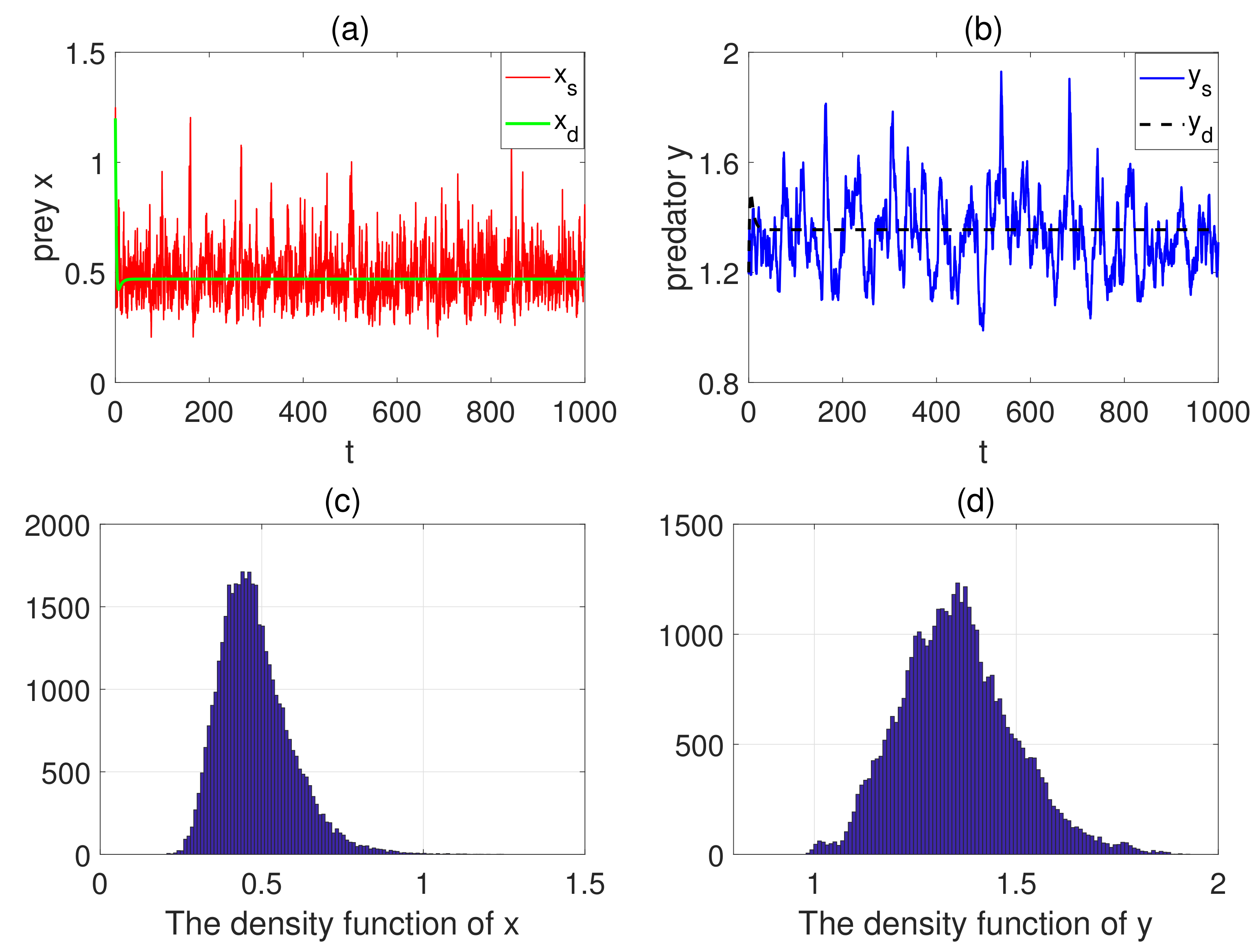
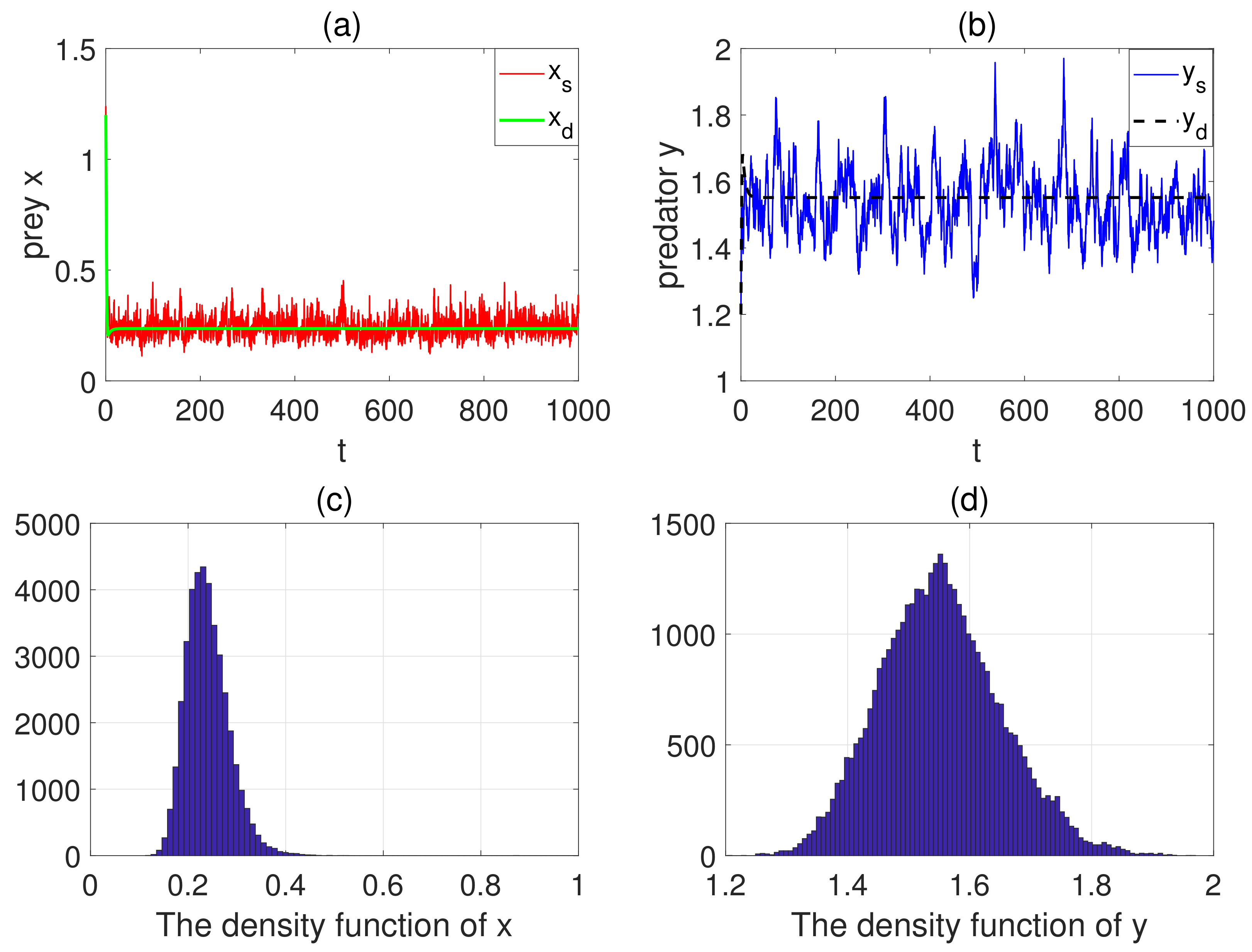
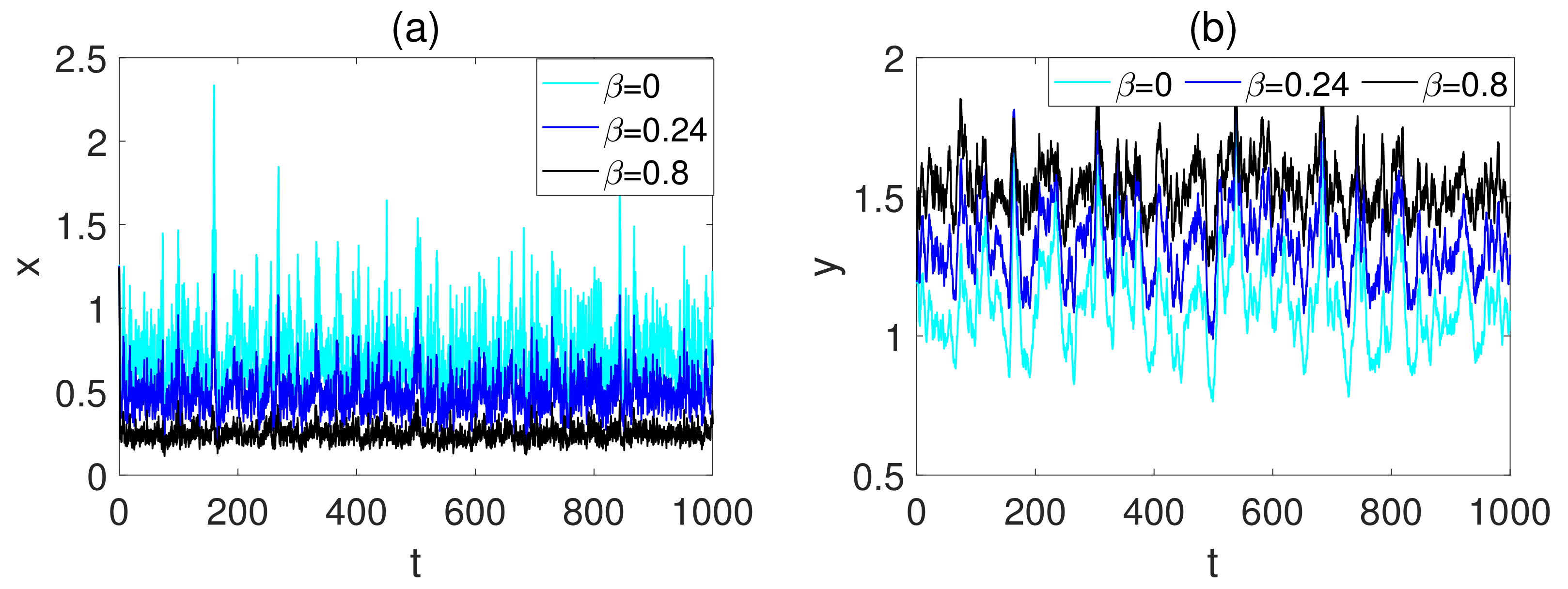
5. Numerical Simulations

In this part, Milstein’s method [36] is used to simulate the conclusions. Considering the following discrete equation

$$\left\{\begin{array}{cc}\hfill x_{k+1}=& x_k+\left[r_0-d_0{x}_k-\frac{\left(\alpha +\beta y_k\right)x_k{y}_k}{1+\delta (\alpha +\beta y_k)x_k}\right]\mathrm{\Delta }t+x_k({\sigma }_{11}+{\sigma }_{12}{x}_k)\sqrt{\mathrm{\Delta }t}{\xi }_k\hfill \\ & +\frac{x_k}{2}\left(2{\sigma }_{11}^2+3{\sigma }_{11}{\sigma }_{12}{x}_k+2{\sigma }_{12}^2{x}_k^2\right)\left({\xi }_k^2-1\right)\mathrm{\Delta }t,\hfill \\ \hfill y_{k+1}=& y_k+\left[\frac{k(\alpha +\beta y_k)x_k{y}_k}{1+\delta (\alpha +\beta y_k)x_k}-d{y}_k\right]\mathrm{\Delta }t+y_k({\sigma }_{21}+{\sigma }_{22}{y}_k)\sqrt{\mathrm{\Delta }t}{\zeta }_k\hfill \\ & +\frac{y_k}{2}\left(2{\sigma }_{21}^2+3{\sigma }_{21}{\sigma }_{22}{y}_k+2{\sigma }_{22}^2{y}_k^2\right)\left({\zeta }_k^2-1\right)\mathrm{\Delta }t,\hfill \end{array}\right.$$

where ${\xi }_k$ and ${\zeta }_k$$(k=1,2,\cdots )$ obey the Gaussian distribution. The next three examples verify the results of this paper.

Case 1: The effect of white noise

In this case, we analyze the impacts of environmental disturbances on the prey and predator populations. Taking the parameter values in

Table 2. The parameter values of model $\left(2\right)$.

Parameter Values	Case 1	Case 2
$r_0$	0.5	0.5
$\beta$	0.24	0.8
$\alpha$	0.6	0.6
$d_0$	0.24	0.24
d	0.2	0.2
$\delta$	1.2	1.2
k	0.7	0.7

. Choosing ${\sigma }_{11}=0.25,{\sigma }_{12}=0.01,{\sigma }_{21}=0.01,{\sigma }_{22}=0.01.$ We can obtain $R_1=0.3833>0$, $R_2=0.336>0$ and $R_0=9.214>1,$ which satisfy the conditions of Theorems 4 and 5, respectively. This indicates the prey and predator populations are persistent (see Figure 1a,b). That is to say, when the white noise is small, it has less effect on the populations at this time. Furthermore, we see that model $\left(2\right)$ exists as a unique stationary distribution (see Figure 1c,d). Keeping the other parameters fixed, let ${\sigma }_{21}=0.01\to 0.9$. Notice that $R_1=-0.0217<0$ holds, which fulfills the condition of Theorem. We find the prey population is persistent (see Figure 2a) and the predator population is extinct (see Figure 2b). This shows the impact of white noise on $y\left(t\right)$ is significant. That is, only the prey population is persistent.

Case 2: The effect of hunting cooperation coefficient $\mathbf{\beta }$.

In this case, we investigate the effects of hunting cooperation on populations. Let $\beta :0.24\to 0.8$, other parameters remain unchanged as Case 1. We obtain $R_1=0.3833>0$, $R_2=0.336>0$ and $R_0=9.214>1$. Through numerical simulation, we deduce that the prey and predator populations are persistent in mean (see Figure 3a,b) and the model $\left(2\right)$ exists as a unique stationary distribution (see Figure 3c,d). Furthermore, we see that as the hunting cooperation coefficient increases, the number of predator population also increases (see Figure 4a,b). That is to say, hunting cooperation is beneficial to the growth of predator populations.

6. Conclusions

Compared to other interrelated papers for deterministic or stochastic predator–prey models with hunting cooperation, this paper considers the dynamic behavior of the model from several aspects. At first, we prove the well-posedness of model $\left(\right)$. Secondly, we prove the extinction and persistence in mean. Moreover, we study the unique stationary ergodic distribution. The influence of nonlinear disturbance on the model is also illustrated. The main results are summarized as follows

(1)

If $R_1=\frac{k}{\delta }-d-\frac{1}{2}{\sigma }_{21}^2<0$ holds, the predator $y\left(t\right)$ can be extinct.

(2)

When $R_1<0$ holds, the prey $x\left(t\right)$ can be persistent and have a unique ergodic stationary distribution.

(3)

When $R_2=k\alpha {\int }_0^{+\infty }\frac{X}{1+\delta \alpha X}\pi \left(X\right)\mathrm{d}X-d-{\sigma }_{21}^2>0$, the predator $y\left(t\right)$ can be persistent in the mean.

(4)

When $R_0=\frac{r_0}{\left(\frac{{\sigma }_{21}^2}{2}+d\right)\left(\frac{{\sigma }_{11}^2}{2}+d_0\right)}>1$, then model $\left(2\right)$ has a unique ergodic stationary distribution.

Besides, through several numerical simulations, we find that environmental disturbance can specifically impact the survival of the prey and predator populations. Even the predator population will become extinct when the noise is high. On the other hand, we discover that hunting cooperation positively affects the predator population. Practical and effective hunting cooperation is beneficial to the survival of the predator population.

In a word, we find that the predation rate is a saturated functional response when $\beta =0$. However, this paper mainly studies the case that $\beta \ne 0$. Figure 4 shows the obvious influence of the predation cooperation coefficient on the model. In addition, according to Lemma 5, Theorem 4 and the construction of V function in proving Theorem 5, we can see the important influence of nonlinear disturbance on the model. Moreover, we overcome the difficulties in the construction of V function and the process of inequality expansion and contraction. The above description improves on previous studies.

References

1. Lotka, A.J. Elements of Physical Biology; Williams and Wilkins: Philadelphia, PA, USA, 1925. [Google Scholar]
2. Volterra, V. Fluctuations in the abundance of a species considered mathematically. Nature 1926, 118, 558–560. [Google Scholar] [CrossRef]
3. Zegeling, A.; Kooij, R.E. Singular perturbations of the Holling I predator-prey system with a focus. J. Differ. Equ. 2020, 269, 5434–5462. [Google Scholar] [CrossRef]
4. Shao, Y. Global stability of a delayed predator-prey system with fear and Holling-type II functional response in deterministic and stochastic environments. Math. Comput. Simul. 2022, 200, 65–77. [Google Scholar] [CrossRef]
5. Dai, Y.; Zhao, Y.; Sang, B. Four limit cycles in a predator-prey system of Leslie type with generalized Holling type III functional response. Nonlinear Anal.-Real World Appl. 2019, 50, 218–239. [Google Scholar] [CrossRef]
6. Lu, C. Dynamical analysis and numerical simulations on a crowley-Martin predator-prey model in stochastic environment. Appl. Math. Comput. 2022, 413, 126641. [Google Scholar] [CrossRef]
7. Zou, X.; Li, Q.; Lv, J. Stochastic bifurcations, a necessary and sufficient condition for a stochastic beddington-deangelis predator-prey model. Appl. Math. Lett. 2021, 117, 107069. [Google Scholar] [CrossRef]
8. Cosner, C.; DeAngelis, D.L.; Ault, J.S.; Olson, D.B. Effects of spatial grouping on the functional response of predators. Theor. Popul. Biol. 1999, 56, 65–75. [Google Scholar] [CrossRef] [PubMed]
9. Rana, S.; Sabyasachi, B.; Sudip, S. Spatiotemporal dynamics of Leslie-Gower predator-prey model with Allee effect on both populations. Math. Comput. Simul. 2022, 200, 32–49. [Google Scholar] [CrossRef]
10. Mukherjee, D.; Maji, C. Bifurcation analysis of a Holling type II predator-prey model with refuge. Chin. J. Phys. 2020, 65, 153–162. [Google Scholar] [CrossRef]
11. Liu, K.; Meng, X.; Chen, L. A new stage structured predator-prey Gomportz model with time delay and impulsive perturbations on the prey. Appl. Math. Comput. 2008, 196, 705–719. [Google Scholar] [CrossRef]
12. Meng, X.; Li, F.; Gao, S. Global analysis and numerical simulations of a novel stochastic eco-epidemiological model with time delay. Appl. Math. Comput. 2018, 339, 701–726. [Google Scholar] [CrossRef]
13. How, M.J.; Santon, M. Cuttlefish camouflage: Blending in by matching background features. Curr. Biol. 2022, 32, R523–R525. [Google Scholar] [CrossRef] [PubMed]
14. Reiter, S.; Laurent, G. Visual perception and cuttlefish camouflage. Curr. Opin. Neurobiol. 2020, 60, 47–54. [Google Scholar] [CrossRef] [PubMed]
15. Niu, Y.; Sun, H.; Stevens, M. Plant camouflage: Ecology, evolution, and implications. Trends Ecol. Evol. 2018, 33, 608–618. [Google Scholar] [CrossRef]
16. Molla, H.; Sarwardi, S.; Haque, M. Dynamics of adding variable prey refuge and an Allee effect to a predator-prey model. Alex. Eng. J. 2022, 61, 4175–4188. [Google Scholar] [CrossRef]
17. Kaur, R.P.; Sharma, A.; Sharma, A.K. Impact of fear effect on plankton-fish system dynamics incorporating zooplankton refuge. Chaos Solitons Fractals 2021, 143, 110563. [Google Scholar] [CrossRef]
18. Al-Salti, N.; Al-Musalhi, F.; Gandhi, V.; Al-Moqbali, M.; Elmojtaba, I. Dynamical analysis of a prey-predator model incorporating a prey refuge with variable carrying capacity. Ecol. Complex. 2021, 45, 100888. [Google Scholar] [CrossRef]
19. Scheel, D.; Packer, C. Group hunting behaviour of lions: A search for cooperation. Anim. Behav. 1991, 41, 697–709. [Google Scholar] [CrossRef]
20. Heinsohn, R.; Packer, C. Complex cooperative strategies in group-territorial African lions. Science 1995, 269, 1260–1262. [Google Scholar] [CrossRef]
21. Schmidt, P.A.; Mech, L.D. Wolf pack size and food acquisition. Am. Nat. 1997, 269, 513–517. [Google Scholar] [CrossRef]
22. Fu, S.; Zhang, H. Effect of hunting cooperation on the dynamic behavior for a diffusive Holling type II predator-prey model. Commun. Nonlinear Sci. Numer. Simul. 2021, 99, 105807. [Google Scholar] [CrossRef]
23. Pal, S.; Pal, N.; Samanta, S.; Chattopadhyay, J. Fear effect in prey and hunting cooperation among predators in a Leslie-Gower model. Math. Biosci. Eng. 2019, 16, 5146–5179. [Google Scholar] [CrossRef] [PubMed]
24. Sk, N.; Tiwari, P.K.; Pal, S. A delay nonautonomous model for the impacts of fear and refuge in a three species food chain model with hunting cooperation. Math. Comput. Simul. 2022, 192, 136–166. [Google Scholar] [CrossRef]
25. Qi, H.; Meng, X.; Hayat, T.; Hobiny, A. Stationary distribution of a stochastic predator-prey model with hunting cooperation. Appl. Math. Lett. 2022, 124, 107662. [Google Scholar] [CrossRef]
26. Zhang, S.; Yuan, S.; Zhang, T. A predator-prey model with different response functions to juvenile and adult prey in deterministic and stochastic environments. Appl. Math. Comput. 2022, 413, 126598. [Google Scholar] [CrossRef]
27. Peng, H.; Zhang, X. The dynamics of stochastic predator-prey models with non-constant mortality rate and general nonlinear functional response. J. Nonlinear Model. Anal. 2020, 2, 495–511. [Google Scholar]
28. Wei, N.; Li, M. Stochastically permanent analysis of a non-autonomous holling II predator-prey model with a complex type of noises. J. Appl. Anal. Comput. 2022, 12, 479–496. [Google Scholar]
29. Qi, H.; Meng, X. Threshold behavior of a stochastic predator-prey system with prey refuge and fear effect. Appl. Math. Lett. 2021, 113, 106846. [Google Scholar] [CrossRef]
30. Qi, H.; Meng, X. Mathematical modeling, analysis and numerical simulation of HIV: The influence of stochastic environmental fluctuations on dynamics. Math. Comput. Simul. 2021, 187, 700–719. [Google Scholar] [CrossRef]
31. Liu, Q.; Jiang, D.; Hayat, T.; Ahmad, B. Stationary distribution and extinction of a stochastic predator-prey model with additional food and nonlinear perturbation. Appl. Math. Comput. 2018, 320, 226–239. [Google Scholar] [CrossRef]
32. Zhao, Y.; Jiang, D. The threshold of a stochastic SIS epidemic model with vaccination. Appl. Math. Comput. 2014, 243, 718–727. [Google Scholar] [CrossRef]
33. Liu, Q.; Jiang, D. Influence of the fear factor on the dynamics of a stochastic predator-prey model. Appl. Math. Lett. 2021, 112, 106756. [Google Scholar] [CrossRef]
34. Asamoah, J.K.K.; Jin, Z.; Sun, G.Q. Non-seasonal and seasonal relapse model for Q fever disease with comprehensive cost-effectiveness analysis. Results Phys. 2021, 22, 103889. [Google Scholar] [CrossRef]
35. Khasminskii, R. Stochastic Stability of Differential Equations, 2nd ed.; Springer: Berlin/Heidelberg, Germany, 2012. [Google Scholar]
36. Omar, M.A.; Aboul-Hassan, A.; Rabia, S.I. The composite Milstein methods for the numerical solution of Ito stochastic differential equations. J. Comput. Appl. Math. 2011, 235, 2277–2299. [Google Scholar] [CrossRef]
Figure 1. (a,b) The persistence of model ( 2 ) . (c,d) The probability density functions of x ( t ) and y ( t ) of model ( 2 ) .
Mathematics 10 02890 g001
Figure 2. (a,b) The paths of prey x ( t ) and predator y ( t ) .
Mathematics 10 02890 g002
Figure 3. (a,b) The persistence of model ( 2 ) with β = 0.8 . (c,d) The probability density functions of x ( t ) and y ( t ) of model ( 2 ) with β = 0.8 .
Mathematics 10 02890 g003
Figure 4. (a,b) The trajectories of x ( t ) and y ( t ) for model ( 2 ) with different hunting cooperation coefficients.
Mathematics 10 02890 g004