Tail Asymptotics for a Retrial Queue with Bernoulli Schedule

Abstract

In this paper, we study the asymptotic behaviour of the tail probability of the number of customers in the steady-state $M/G/1$ retrial queue with Bernoulli schedule, under the assumption that the service time distribution has a regularly varying tail. Detailed tail asymptotic properties are obtained for the conditional probability of the number of customers in the (priority) queue and orbit, respectively, in terms of the recently proposed exhaustive stochastic decomposition approach. Numerical examples are presented to show the impacts of system parameters on the tail asymptotic probabilities.

1. Introduction

As one of the important types of queueing systems, retrial queues have been extensively studied for more than 40 years and hundreds of literature publications have been produced. Research on retrial queues is still very active due to continuously emerging new challenges. A general picture of retrial models, together with their applications in various areas, and basic results on retrial queues can be acquired from books or recent surveys, such as Falin and Templeton [1], Artajelo and Gómez-Corral [2], Choi and Chang [3], Kim and Kim [4], Phung-Duc [5], among possible others.

Tail asymptotic analysis of retrial queueing systems, especially asymptotic properties in tail stationary probabilities for a stable retrial queue, has been a focus of the investigation in the past 10 years or so, due to two main reasons: first, for most of retrial queues, it is not expected to have explicit non-transform solutions for their stationary distributions, and, second, tail asymptotic properties often lead to approximations to performance metrics and numerical algorithms. Both light-tailed and heavy-tailed properties have been obtained for a number of retrial queues, including the following incomplete list: Kim, Kim and Ko [6], Liu and Zhao [7], Kim, Kim and Kim [8], Liu, Wang and Zhao [9], Kim and Kim [10], Artalejo and Phung-Duc [11], Walraevens, Claeys and Phung-Duc [12], Kim, Kim and Kim [13], Yamamuro [14], Masuyama [15], Liu, Min and Zhao [16], and Liu and Zhao [17].

In this paper, we consider an $M/G/1$ retrial queue with a Bernoulli schedule. This model was first proposed and studied by Choi and Park [18], but tail asymptotic behaviour was not a focus of the study. This $M/G/1$ retrial queueing system consists of a (priority) queue of infinite waiting capacity and an orbit. External customers arrive to this system according to a Poisson process with rate $\lambda$. There is a single server in this system. If the server is idle upon the arrival of a customer, the customer receives the service immediately and leaves the system after the completion of the service. Otherwise, if the server is busy, the arriving customer would join the queue with probability q, becoming a priority customer waiting for the service according to the first-in-first-out discipline; or the orbit with probability $p=1-q$, becoming a repeated customer who will retry later for receiving its service, which is referred to as the Bernoulli scheduling. A priority customer has priority over a repeated customer for receiving the service. This implies that, upon the completion of a service, if there is a customer in the queue, the server will serve the customer at the head of the queue; otherwise, the server becomes idle. Each of the repeated customers in the orbit independently repeatedly tries to receive service, according to a Poisson process with the retrial rate $\mu$, until an idle server is found, and then immediately receives its service. Upon the completion of the service, the customer leaves the system. Service times for all customers are i.i.d. random variables. By $T_{\beta }$, we denote the generic service time whose distribution $F_{\beta }\left(x\right)$ with $F_{\beta }\left(0\right)=0$ is assumed to have a finite mean ${\beta }_1$. The Laplace–Stieltjes transform (LST) of the distribution function $F_{\beta }\left(x\right)$ is denoted by $\beta \left(s\right)$. Our interest in this paper is the tail stationary asymptotic behaviour for this system with the following assumption on the heavy-tailed service time:

Assumption 1.

The service time $T_{\beta }$ has tail probability $P\{T_{\beta }>t\}\sim t^{-a}L\left(t\right)$ as $t\to \infty$, where $a>1$, and $L\left(t\right)$ is a slowly varying function at ∞ (see Definition A1).

It should be noted that this assumption is different from that made in [17], where the low priority customers have the tail probabilities lighter than the high priority customers. Therefore, the study carried out in this paper is not overlapped with that in [17].

We also mention some literature studies on similar models to that considered in [18], such as Falin, Artalejo, and Martin [19], in which a model with two independent (primary) Poisson arrival streams was considered. The priority customers, when blocked upon arrival, are queued and waiting for service, while the non-priority customers, when blocked, join the orbit and retry for service later; Li and Yang [20], in which the discrete-time counterpart to the model studied in this paper, or a Geo/G/1 retrial queue with Bernoulli schedule, was considered; and Atencia and Moreno [21], in which the $M/G/1$ retrial queueing system with Bernoulli schedule has a general retrial time, but only the customer at the head of the orbit is allowed to retry for service, or retrials with a constant rate. Once again, our focus and also the method in the study are different from those in the above mentioned studies.

Let ${\lambda }_1=\lambda q$, ${\lambda }_2=\lambda p$, ${\rho }_1={\lambda }_1{\beta }_1$, ${\rho }_2={\lambda }_2{\beta }_1$ and $\rho ={\rho }_1+{\rho }_2=\lambda {\beta }_1$. It follows from [18] that the system considered in this paper is stable if and only if (iff) $\rho <1$, which is assumed to hold throughout the paper. For obtaining asymptotic properties in various tail stationary probabilities of this $M/G/1$ retrial queue with Bernoulli schedule, which is the focus of this paper, we start with two expressions for probability transformations obtained in [18]. The method employed in our analysis is the exhaustive stochastic decomposition, recently proposed in [17]. By assuming a regular varying tail in the service time distribution, as made in Assumption A, we obtain asymptotic properties for the conditional tail probabilities of customers:

(1)

in the orbit, given that the server is idle (Section 4.1);

(2)

in the queue, given that the server is busy (Section 4.2); and

(3)

in the orbit, given that the server is busy (Section 4.3).

Numerical curves are presented to demonstrate how system parameters, say the arrival rate, the expected service time or the retrial rate, impact the tail asymptotic probabilities.

The rest of this paper is organized as follows: preliminary results are provided in Section 2; exhaustive stochastic decompositions are obtained in Section 3; and the main results on asymptotic properties for tail probabilities are derived in Section 4; numerical examples are presented in Section 5; and conclusions are made in the final section.

2. Preliminaries

Assume that the system is in steady state. Let $R_{que}$ be the number of priority customers in the queue, excluding the possible one in the service, let $R_{orb}$ be the number of repeated customers in the orbit, and let $I_{ser}=1$ or 0, whenever the server is busy or idle, respectively. Let $R_0$ be a random variable (r.v.) whose distribution coincides with the conditional distribution of $R_{orb}$, given that $I_{ser}=0$, and let $(R_{11},R_{12})$ be a two-dimensional r.v. whose distribution coincides with the conditional distribution of $(R_{que},R_{orb})$, given that $I_{ser}=1$. Precisely, $R_0$, $R_{11}$, and $R_{12}$ are all nonnegative integer-valued r.v.s; and $R_0$ has the probability generating function (PGF) $R_0\left(z_2\right)=E\left(z_2^{R_0}\right)\stackrel{def}{=}E(z_2^{R_{orb}}\mid I_{ser}=0)$ and $(R_{11},R_{12})$ has the PGF $R_1(z_1,z_2)=E\left(z_1^{R_{11}}{z}_2^{R_{12}}\right)\stackrel{def}{=}E(z_1^{R_{que}}{z}_2^{R_{orb}}\mid I_{ser}=1)$.

Our starting point for tail asymptotic analysis is based on the expressions for $R_0\left(z_2\right)$ and $R_1(z_1,z_2)$. Following the discussions in [18], let

$$\begin{array}{ccc}\hfill M_a(z_1,z_2)& =& \frac{1}{\rho }·\frac{1-\beta (\lambda -{\lambda }_1{z}_1-{\lambda }_2{z}_2)}{1-p{z}_2-q{z}_1},\hfill \end{array}$$

(1)

$$\begin{array}{ccc}\hfill M_b(z_1,z_2)& =& (1-{\rho }_1)·\frac{h\left(z_2\right)-z_1}{\beta (\lambda -{\lambda }_1{z}_1-{\lambda }_2{z}_2)-z_1},\hfill \end{array}$$

(2)

$$\begin{array}{ccc}\hfill M_c\left(z_2\right)& =& \frac{1-\rho }{1-{\rho }_1}·\frac{1-z_2}{h\left(z_2\right)-z_2},\hfill \end{array}$$

(3)

where $h(·)$ is determined uniquely by the following equation:

$$h\left(z\right)=\beta (\lambda -{\lambda }_{1}h\left(z\right)-{\lambda }_{2}z).$$

(4)

Since $P\{I_{ser}=0\}=1-\rho$ and $P\{I_{ser}=1\}=\rho$, obtained in [18], we have the following expressions immediately from Equations (12) and (13) in [18]:

$$\begin{array}{ccc}\hfill R_0\left(z_2\right)& =& exp\left\{-\frac{\lambda }{\mu }{\int }_{z_2}^1\frac{1-h\left(u\right)}{h\left(u\right)-u}du\right\},\hfill \end{array}$$

(5)

$$\begin{array}{ccc}\hfill R_1(z_1,z_2)& =& M_a(z_1,z_2)·M_b(z_1,z_2)·M_c\left(z_2\right)·R_0\left(z_2\right).\hfill \end{array}$$

(6)

Next, we provide a probabilistic interpretation for $h\left(z\right)$ in (4). Let $T_{\alpha }$ be the busy period of the standard $M/G/1$ queue (without retrial) with arrival rate ${\lambda }_1$ and service time $T_{\beta }$. By $F_{\alpha }\left(x\right)$, we denote the probability distribution function of $T_{\alpha }$, and by $\alpha \left(s\right)$, the LST of $F_{\alpha }\left(x\right)$. The following are classic results on the busy period of this standard $M/G/1$ queue (referring, e.g., to [22]):

$$\begin{array}{ccc}\hfill \alpha \left(s\right)& =& \beta (s+{\lambda }_1-{\lambda }_1\alpha \left(s\right)),\hfill \end{array}$$

(7)

$$\begin{array}{ccc}\hfill {\alpha }_1& \stackrel{\mathrm{def}}{=}& E\left(T_{\alpha }\right)={\beta }_1/(1-{\rho }_1).\hfill \end{array}$$

(8)

Throughout this paper, we use the notation $N_b\left(t\right)$ to represent the number of Poisson arrivals, with rate b, within the time interval $(0,t]$, and $N_{{\lambda }_2}\left(T_{\alpha }\right)$ to represent the number of arrivals of a Poisson process, with arrival rate ${\lambda }_2$, within the independent random time $T_{\alpha }$. The PGF of $N_{{\lambda }_2}\left(T_{\alpha }\right)$ is easily obtained as follows:

$$E\left(z^{N_{{\lambda }_2}\left(T_{\alpha }\right)}\right)={\int }_0^{\infty }\sum _{n=0}^{\infty }{z}^n\frac{{\left({\lambda }_{2}x\right)}^n}{n!}{e}^{-{\lambda }_{2}x}d{F}_{\alpha }\left(x\right)=\alpha ({\lambda }_2-{\lambda }_{2}z).$$

(9)

It follows from (7) that

$$\alpha ({\lambda }_2-{\lambda }_{2}z)=\beta (\lambda -{\lambda }_1\alpha ({\lambda }_2-{\lambda }_{2}z)-{\lambda }_{2}z).$$

(10)

By comparing (4) and (10), and noticing the uniqueness of $h\left(z\right)$, we immediately have

$$h\left(z\right)=\alpha ({\lambda }_2-{\lambda }_{2}z)=E\left(z^{N_{{\lambda }_2}\left(T_{\alpha }\right)}\right).$$

(11)

Remark 1.

$h\left(z\right)$ is the PGF of the number of arrivals of a Poisson process with arrival rate ${\lambda }_2$ within an independent random time $T_{\alpha }$, where $T_{\alpha }$ has the same probability distribution as that for the busy period of the standard $M/G/1$ queue with arrival rate ${\lambda }_1$ and service time $T_{\beta }$.

Since $T_{\alpha }$ is the busy period of the standard $M/G/1$ queue with arrival rate ${\lambda }_1$ and the service time $T_{\beta }$, its asymptotic tail probability is regularly varying according to de Meyer and Teugels [22] (see Lemma A1 in Appendix A).

3. Exhaustive Stochastic Decompositions

In this section, we verify that $R_0\left(z_2\right)$ can be viewed as the PGF of a r.v., which is written in a form of stochastic decompositions. The result will be used for the asymptotic analysis in later sections.

Based on the definition of $R_0$ given earlier, this is a r.v. whose distribution coincides with the conditional distribution of $R_{orb}$, given that $I_{ser}=0$. In this section, we provide a new probabilistic interpretation for $R_0$, which is useful for our tail asymptotic analysis.

Substituting (11) into (5), we have

$$R_0\left(z_2\right)=exp\left\{-\frac{\lambda }{\mu }{\int }_{z_2}^1\frac{1-\alpha ({\lambda }_2-{\lambda }_{2}u)}{\alpha ({\lambda }_2-{\lambda }_{2}u)-u}du\right\}.$$

(12)

In order to rewrite (12), we let

$$\begin{array}{ccc}\hfill \psi & =& \frac{\rho }{\mu (1-\rho )},\hfill \end{array}$$

(13)

$$\begin{array}{ccc}\hfill \kappa \left(s\right)& =& \frac{1-\rho }{{\beta }_1}·\frac{1-\alpha \left(s\right)}{s-{\lambda }_2+{\lambda }_2\alpha \left(s\right)},\hfill \end{array}$$

(14)

$$\begin{array}{ccc}\hfill \omega \left(s\right)& =& 1-{\int }_0^s\kappa \left(u\right)du,\hfill \end{array}$$

(15)

$$\begin{array}{ccc}\hfill \tau \left(s\right)& =& exp\left\{\psi \omega \left(s\right)-\psi \right\}.\hfill \end{array}$$

(16)

From (12)–(16),

$$\begin{array}{ccc}\hfill R_0\left(z_2\right)& =& exp\left\{-\frac{\lambda }{\mu }{\int }_0^{{\lambda }_2-{\lambda }_2{z}_2}\frac{1-\alpha \left(s\right)}{s-{\lambda }_2+{\lambda }_2\alpha \left(s\right)}ds\right\}\hfill \\ & =& exp\left\{-\psi {\int }_0^{{\lambda }_2-{\lambda }_2{z}_2}\kappa \left(u\right)du\right\}\hfill \\ & =& \tau ({\lambda }_2-{\lambda }_2{z}_2).\hfill \end{array}$$

(17)

In the following three remarks, we assert that $\kappa \left(s\right)$, $\omega \left(s\right)$ and $\tau \left(s\right)$ are the LSTs of three probability distribution functions on $[0,\infty )$, respectively. For the first assertion, let $F_{\alpha }^{\left(e\right)}\left(x\right)$ be the equilibrium distribution of $F_{\alpha }\left(x\right)$, which is defined as $F_{\alpha }^{\left(e\right)}\left(x\right)={\alpha }_1^{-1}{\int }_0^x(1-F_{\alpha }\left(t\right))dt$, where ${\alpha }_1=E\left(T_{\alpha }\right)$ is given in (8). The LST of $F_{\alpha }^{\left(e\right)}\left(x\right)$ can be written as ${\alpha }^{\left(e\right)}\left(s\right)=(1-\alpha \left(s\right))/\left({\alpha }_{1}s\right)$. From (14), we have

$$\kappa \left(s\right)=\frac{(1-\vartheta ){\alpha }^{\left(e\right)}\left(s\right)}{1-\vartheta {\alpha }^{\left(e\right)}\left(s\right)}=\sum _{k=1}^{\infty }(1-\vartheta ){\vartheta }^{k-1}{\left({\alpha }^{\left(e\right)}\left(s\right)\right)}^k,$$

(18)

where

$$\vartheta ={\lambda }_2{\alpha }_1={\rho }_2/(1-{\rho }_1)<1.$$

(19)

Remark 2.

Immediately from (18), $\kappa \left(s\right)$ can be viewed as the LST of the distribution function of a r.v. $T_{\kappa }$, whose distribution function is denoted by $F_{\kappa }\left(x\right)$. More precisely, $T_{\kappa }\stackrel{\mathrm{d}}{=}{T}_{\alpha ,1}^{\left(e\right)}+T_{\alpha ,2}^{\left(e\right)}+\cdots +T_{\alpha ,J}^{\left(e\right)}$, where $T_{\alpha ,j}^{\left(e\right)}$, $j\ge 1$ are i.i.d. r.v.s, each with the distribution $F_{\alpha }^{\left(e\right)}\left(x\right)$, $P(J=j)=(1-\vartheta ){\vartheta }^{j-1}$, $j\ge 1$, and J is independent of $T_{\alpha ,j}^{\left(e\right)}$ for $j\ge 1$. In the above expression, and also later, the notation “$\stackrel{\mathrm{d}}{=}$” stands for equality in probability distribution.

For the second assertion, we will use Theorem 1 in Feller [23] (see p. 439): A function $\phi \left(s\right)$ is the LST of a probability distribution function iff $\phi \left(0\right)=1$ and $\phi \left(s\right)$ is completely monotone, i.e., $\phi \left(s\right)$ possesses derivatives ${\phi }^{\left(n\right)}\left(s\right)$ of all orders such that ${(-1)}^n{\phi }^{\left(n\right)}\left(s\right)\ge 0$ for $s>0$.

Remark 3.

Immediately from (15), $\omega \left(0\right)=1$ and ${(-1)}^n{\omega }^{\left(n\right)}\left(s\right)={(-1)}^{n-1}{\kappa }^{(n-1)}\left(s\right)\ge 0$ for $s>0$, which implies that $\omega \left(s\right)$ is the LST of the probability distribution function of a r.v. $T_{\omega }$, whose distribution is denoted by $F_{\omega }\left(x\right)$.

For the third assertion, we write (16) as

$$\tau \left(s\right)=\sum _{k=0}^{\infty }\frac{{\psi }^k}{k!}{e}^{-\psi }{\left(\omega \left(s\right)\right)}^k.$$

(20)

Remark 4.

Immediately from (20), $\tau \left(s\right)$ can be viewed as the LST of the distribution function of a r.v. $T_{\tau }$, whose distribution function is denoted by $F_{\tau }\left(x\right)$. More precisely, $T_{\tau }\stackrel{\mathrm{d}}{=}{\sum }_{j=0}^J{T}_{\omega ,j}$, where $T_{\omega ,j}$, $j\ge 1$, are i.i.d. r.v.s each with the distribution $F_{\omega }\left(x\right)$, and $P(J=j)=\frac{{\psi }^j}{j!}{e}^{-\psi }$, $j\ge 0$, where J is independent of $T_{\omega ,j}$ for $j\ge 0$.

The following remark provides a detailed interpretation on (17).

Remark 5.

$R_0$ can be regarded as the number of Poisson arrivals with rate ${\lambda }_2$ within an independent random time $T_{\tau }$, i.e., $R_0\stackrel{\mathrm{d}}{=}{N}_{{\lambda }_2}\left(T_{\tau }\right)$.

4. Tail Asymptotics

In this section, we will study the asymptotic behaviour for the tail probabilities $P\{R_{orb}>j\mid I_{ser}=0\}$, $P\{R_{que}>j\mid I_{ser}=1\}$ and $P\{R_{orb}>j\mid I_{ser}=1\}$, as $j\to \infty$, respectively.

4.1. Asymptotic Tail Probability for $P\{R_{orb}>j\mid I_{ser}=0\}$

To study the asymptotic behaviour for the tail probability $P\{R_{orb}>j\mid I_{ser}=0\}\equiv P\{R_0>j\}$, let us first study the asymptotic properties of the tail probabilities for $T_{\kappa }$, $T_{\omega }$ and $T_{\tau }$, respectively.

By Lemma A1, we know that $P\{T_{\alpha }>t\}\sim {(1-{\rho }_1)}^{-a-1}{t}^{-a}L\left(t\right)$ as $t\to \infty$, where the r.v. $T_{\alpha }$ is the busy period defined in Section 2. Applying Karamata’s theorem (e.g., p. 28 in [24]), we have ${\int }_t^{\infty }(1-F_{\alpha }\left(x\right))dx\sim {(a-1)}^{-1}{(1-{\rho }_1)}^{-a-1}{t}^{-a+1}L\left(t\right)$, which implies that $1-F_{\alpha }^{\left(e\right)}\left(t\right)\sim {\left((a-1){\alpha }_1\right)}^{-1}{(1-{\rho }_1)}^{-a-1}{t}^{-a+1}L\left(t\right)$, $t\to \infty$. By Remark 2 and applying Lemma A2, we obtain the following tail asymptotic property for $T_{\kappa }$.

Lemma 1.

$$\begin{array}{ccc}\hfill P\{T_{\kappa }>t\}& \sim & c_{\kappa }·t^{-a+1}L\left(t\right),t\to \infty ,\hfill \end{array}$$

(21)

where

$$\begin{array}{c}\hfill c_{\kappa }=\frac{1}{{\alpha }_1(1-\vartheta )(a-1){(1-{\rho }_1)}^{a+1}}=\frac{1}{{\beta }_1(1-\rho )(a-1){(1-{\rho }_1)}^{a-1}}.\end{array}$$

(22)

In the following lemma, we present the asymptotic tail probability of $T_{\omega }$.

Lemma 2.

$$P\{T_{\omega }>t\}\sim (1-1/a)c_{\kappa }·t^{-a}L\left(t\right),t\to \infty .$$

(23)

Proof. 

Recall that $T_{\omega }$ has the distribution function $F_{\omega }\left(x\right)$, defined in terms of its LST $\omega \left(s\right)$ in (15), which is determined by the LST $\kappa \left(s\right)$ of the distribution function of $T_{\kappa }$. We divide the proof into two parts, depending on whether a is an integer or not.

• Case 1: Non-integer $a>1$.

Suppose that $m<a<m+1$, $m\in \{1,2,\dots \}$. Since $P\{T_{\kappa }>t\}\sim c_{\kappa }·t^{-a+1}L\left(t\right)$, we have its moments ${\kappa }_{m-1}<\infty$ and ${\kappa }_m=\infty$. Define ${\kappa }_{m-1}\left(s\right)$ in a manner similar to that in (A3). Then, $\kappa \left(s\right)={\sum }_{k=0}^{m-1}\frac{{\kappa }_k}{k!}{(-s)}^k+{(-1)}^m{\kappa }_{m-1}\left(s\right)$. By Lemma A5, we know that

$${\kappa }_{m-1}\left(s\right)\sim \left[\mathsf{\Gamma }(a-m)\mathsf{\Gamma }(m+1-a)/\mathsf{\Gamma }(a-1)\right]·c_{\kappa }{s}^{a-1}L(1/s),s\downarrow 0.$$

(24)

From (15), there are constants $\{v_k;k=0,1,2,\dots ,m\}$ satisfying $\omega \left(s\right)={\sum }_{k=0}^m{v}_k{(-s)}^k+{(-1)}^{m+1}{\int }_0^s{\kappa }_{m-1}\left(u\right)du.$ Define ${\omega }_m\left(s\right)$ in a manner similar to that in (A3). Then,

$${\omega }_m\left(s\right)={\int }_0^s{\kappa }_{m-1}\left(u\right)du\sim \left[\mathsf{\Gamma }(a-m)\mathsf{\Gamma }(m+1-a)/\mathsf{\Gamma }\left(a\right)\right]·\frac{a-1}{a}{c}_{\kappa }{s}^{a}L(1/s),s\downarrow 0,$$

(25)

where we have used (24) and Karamata’s theorem (p. 28 in [24]). Applying Lemma A5, we complete the proof of Lemma 2 for non-integer $a>1$.

• Case 2: Integer $a>1$.

Suppose that $a=m\in \{2,3,\dots \}$. Since $P\{T_{\kappa }>t\}\sim c_{\kappa }·t^{-m+1}L\left(t\right)$ implies that $T_{\kappa }$ has its moment ${\kappa }_{m-2}<\infty$, we can define ${\kappa }_{m-2}\left(s\right)$ and ${\widehat{\kappa }}_{m-2}\left(s\right)$ in a manner similar to that in (A3) and (A4), respectively. Then, $\kappa \left(s\right)={\sum }_{k=0}^{m-2}\frac{{\kappa }_k}{k!}{(-s)}^k+{(-1)}^{m-1}{\kappa }_{m-2}\left(s\right)$. By Lemma A6, we obtain

$${\widehat{\kappa }}_{m-2}\left(xu\right)-{\widehat{\kappa }}_{m-2}\left(u\right)\sim -(logx)c_{\kappa }L(1/u)/(m-2)!asu\downarrow 0.$$

(26)

From (15), there exist constants $\{v_k;k=0,1,2,\dots ,m-1\}$ satisfying $\omega \left(s\right)={\sum }_{k=0}^{m-1}{v}_k{(-s)}^k+{(-1)}^m{\int }_0^s{\kappa }_{m-2}\left(u\right)du.$ Define ${\widehat{\omega }}_{m-1}\left(s\right)$ in a manner similar to that in (A4). Then, we have

$${\widehat{\omega }}_{m-1}\left(s\right)=\frac{1}{s^m}{\int }_0^s{u}^{m-1}{\widehat{\kappa }}_{m-2}\left(u\right)du,$$

(27)

which immediately gives us ${\widehat{\omega }}_{m-1}\left(xs\right)=\frac{1}{s^m}{\int }_0^s{u}^{m-1}{\widehat{\kappa }}_{m-2}\left(xu\right)du$. It follows that

$$\begin{array}{ccc}\hfill {\widehat{\omega }}_{m-1}\left(xs\right)-{\widehat{\omega }}_{m-1}\left(s\right)& =& \frac{1}{s^m}{\int }_0^s{u}^{m-1}\left[{\widehat{\kappa }}_{m-2}\left(xu\right)-{\widehat{\kappa }}_{m-2}\left(u\right)\right]du\hfill \\ & \sim & -\frac{m-1}{m}{c}_{\kappa }logx\frac{L(1/s)}{(m-1)!}ass\downarrow 0,\hfill \end{array}$$

(28)

where we have used (26) and Karamata’s theorem (p. 28 in [24]). By applying Lemma A6, we complete the proof of Lemma 2 for integer $a=m\in \{2,3,\dots \}$. □

For the tail asymptotic property of $T_{\tau }$, recall Remark 4, with $T_{\tau }\stackrel{\mathrm{d}}{=}{\sum }_{j=0}^J{T}_{\omega ,j}$, where J has a Poisson distribution with parameter $\psi$, $T_{\omega ,j}$, $j\ge 1$, are i.i.d. r.v.s with the distribution function $F_{\omega }\left(x\right)$, and J is independent of $T_{\omega ,j}$, $j\ge 1$. Then, by Lemmas A2 and 2, we have the following property.

Lemma 3.

$$P\{T_{\tau }>t\}\sim \psi ·P\{T_{\omega }>t\}\sim (1-1/a)c_{\kappa }\psi ·t^{-a}L\left(t\right),t\to \infty .$$

(29)

Now, the asymptotic tail probability for $P\{R_{orb}>j\mid I_{ser}=0\}$ can be obtained based on Lemma 3. From Remark 5, we know that $R_0=N_{{\lambda }_2}\left(T_{\tau }\right)$. Lemma A3 leads to:

$$P\{R_{orb}>j\mid I_{ser}=0\}=P\{R_0>j\}\sim P\{T_{\tau }>j/{\lambda }_2\}\sim \frac{\lambda {\lambda }_2^a}{a\mu {(1-\rho )}^2{(1-{\rho }_1)}^{a-1}}·j^{-a}L\left(j\right),j\to \infty .$$

(30)

4.2. Asymptotic Tail Probability for $P\{R_{que}>j\mid I_{ser}=1\}$

In this subsection, we will study the asymptotic behaviour of the tail probability $P\{R_{que}>j\mid I_{ser}=1\}\equiv P\{R_{11}>j\}$ as $j\to \infty$. For this purpose, we examine the generating function $E\left(z_1^{R_{11}}\right)$ of $R_{11}$. Note that $E\left(z_1^{R_{11}}\right)=R_1(z_1,1)$. Taking $z_2\to 1$ in (3), (5) and (6) and using the fact that $\frac{d}{dz}h\left(z\right){\mid }_{z=1}={\lambda }_2{\alpha }_1={\rho }_2/(1-{\rho }_1)$, we immediately have $M_c\left(1\right)=1$, $R_0\left(1\right)=1$ and

$$E\left(z_1^{R_{11}}\right)=M_a(z_1,1)M_b(z_1,1).$$

(31)

It follows from (1) and (2) that

$$\begin{array}{ccc}\hfill M_a(z_1,1)& =& \frac{1}{{\rho }_1}·\frac{1-\beta ({\lambda }_1-{\lambda }_1{z}_1)}{1-z_1},\hfill \end{array}$$

(32)

$$\begin{array}{ccc}\hfill M_b(z_1,1)& =& \frac{(1-{\rho }_1)(1-z_1)}{\beta ({\lambda }_1-{\lambda }_1{z}_1)-z_1}.\hfill \end{array}$$

(33)

Denote $F_{\beta }^{\left(e\right)}\left(x\right)$ to be the equilibrium distribution of $F_{\beta }\left(x\right)$, that is, $F_{\beta }^{\left(e\right)}\left(x\right)={\beta }_1^{-1}{\int }_0^x(1-F_{\beta }\left(t\right))dt.$ The LST of $F_{\beta }^{\left(e\right)}\left(x\right)$ can be written as ${\beta }^{\left(e\right)}\left(s\right)=(1-\beta \left(s\right))/\left({\beta }_{1}s\right)$. We now have

$$\begin{array}{ccc}\hfill M_a(z_1,1)& =& {\beta }^{\left(e\right)}({\lambda }_1-{\lambda }_1{z}_1),\hfill \end{array}$$

(34)

$$\begin{array}{ccc}\hfill M_b(z_1,1)& =& \frac{1-{\rho }_1}{1-{\rho }_1{\beta }^{\left(e\right)}({\lambda }_1-{\lambda }_1{z}_1)}=\sum _{n=0}^{\infty }(1-{\rho }_1){\rho }_1^n{\left({\beta }^{\left(e\right)}({\lambda }_1-{\lambda }_1{z}_1)\right)}^n.\hfill \end{array}$$

(35)

Substituting (34) and (35) into (31), we have

$$E\left(z_1^{R_{11}}\right)=\xi ({\lambda }_1-{\lambda }_1{z}_1),$$

(36)

where

$$\xi \left(s\right)=\sum _{n=1}^{\infty }(1-{\rho }_1){\rho }_1^{n-1}{\left({\beta }^{\left(e\right)}\left(s\right)\right)}^n.$$

(37)

Remark 6.

Immediately from (37), $\xi \left(s\right)$ can be viewed as the LST of the distribution function of the r.v. $T_{\xi }\stackrel{\mathrm{d}}{=}{T}_{\beta ,1}^{\left(e\right)}+T_{\beta ,2}^{\left(e\right)}+\cdots +T_{\beta ,J}^{\left(e\right)}$, where $T_{\beta ,j}^{\left(e\right)}$, $j\ge 1$, are i.i.d. r.v.s. with a common distribution $F_{\beta }^{\left(e\right)}\left(x\right)$, $P(J=j)=(1-{\rho }_1){\rho }_1^{j-1}$, $j\ge 1$, and J is independent of $T_{\beta ,j}^{\left(e\right)}$, $j\ge 1$.

Under Assumption A, by Karamata’s theorem (e.g., p. 28 in [24]), we have ${\int }_t^{\infty }(1-F_{\beta }\left(x\right))dx\sim {(a-1)}^{-1}{t}^{-a+1}L\left(t\right)$, which implies that $1-F_{\beta }^{\left(e\right)}\left(t\right)\sim {\left((a-1){\beta }_1\right)}^{-1}{t}^{-a+1}L\left(t\right)$, $t\to \infty$. By Remark 6 and applying Lemma A2, we have

$$P\{T_{\xi }>t\}\sim \frac{1}{(1-{\rho }_1)(a-1){\beta }_1}·t^{-a+1}L\left(t\right),t\to \infty .$$

(38)

Remark 7.

With (36), one can interpret $R_{11}$ as the number of Poisson arrivals with rate ${\lambda }_1$ within the independent random time $T_{\xi }$, i.e., $R_{11}\stackrel{\mathrm{d}}{=}{N}_{{\lambda }_1}\left(T_{\xi }\right)$.

By Remark 7 and applying Lemma A3, we have

$$P\{R_{que}>j\mid I_{ser}=1\}=P\{R_{11}>j\}\sim P\{T_{\xi }>j/{\lambda }_1\}\sim \frac{{\lambda }_1^{a-1}}{(1-{\rho }_1)(a-1){\beta }_1}·j^{-a+1}L\left(j\right),j\to \infty .$$

(39)

4.3. Asymptotic Tail Probability for $P\{R_{orb}>j\mid I_{ser}=1\}$

In this subsection, we will study the asymptotic behaviour of the tail probability $P\{R_{orb}>j\mid I_{ser}=1\}\equiv P\{R_{12}>j\}$ as $j\to \infty$. By (6),

$$\begin{array}{c}\hfill E\left(z_2^{R_{12}}\right)=R_1(1,z_2)=M_a(1,z_2)·M_b(1,z_2)·M_c\left(z_2\right)·R_0\left(z_2\right).\end{array}$$

(40)

Taking $z_1\to 1$ in (1)–(3), we have

$$\begin{array}{ccc}\hfill M_a(1,z_2)·M_b(1,z_2)·M_c\left(z_2\right)& =& \frac{1-\rho }{{\rho }_2}·\frac{1-h\left(z_2\right)}{h\left(z_2\right)-z_2}.\hfill \\ & =& \frac{1-\rho }{{\rho }_2}·\frac{1-\alpha ({\lambda }_2-{\lambda }_2{z}_2)}{\alpha ({\lambda }_2-{\lambda }_2{z}_2)-z_2}\left(by\left(11\right)\right)\hfill \end{array}$$

(41)

$$\begin{array}{ccc}& =& \kappa ({\lambda }_2-{\lambda }_2{z}_2),\hfill \end{array}$$

(42)

where the last equality follows from (14).

Substituting (42) and (17) into (40), we have

$$\begin{array}{ccc}\hfill E\left(z_2^{R_{12}}\right)& =& \kappa ({\lambda }_2-{\lambda }_2{z}_2)·\tau ({\lambda }_2-{\lambda }_2{z}_2).\hfill \end{array}$$

(43)

Remark 8.

With (43), one can interpret $R_{12}$ as the number of Poisson arrivals with rate ${\lambda }_2$ within an independent random time $T_{\kappa }+T_{\tau }$, i.e., $R_{12}\stackrel{\mathrm{d}}{=}{N}_{{\lambda }_2}(T_{\kappa }+T_{\tau })$, where $T_{\kappa }$ and $T_{\tau }$ are assumed to be independent.

By (21) and (29), and applying Lemma A4, we have

$$P\{T_{\kappa }+T_{\tau }>t\}\sim P\{T_{\kappa }>t\}\sim c_{\kappa }·t^{-a+1}L\left(t\right),t\to \infty .$$

(44)

Applying Remark 8 and Lemma A3, we have

$$\begin{array}{cc}\hfill P\{R_{orb}>j\mid I_{ser}=1\}=& P\{R_{12}>j\}\sim P\{T_{\kappa }+T_{\tau }>j/{\lambda }_2\}\hfill \\ \hfill \sim & \frac{{\lambda }_2^{a-1}}{{\beta }_1(1-\rho )(a-1){(1-{\rho }_1)}^{a-1}}·j^{-a+1}L\left(j\right),j\to \infty .\hfill \end{array}$$

(45)

5. Numerical Examples

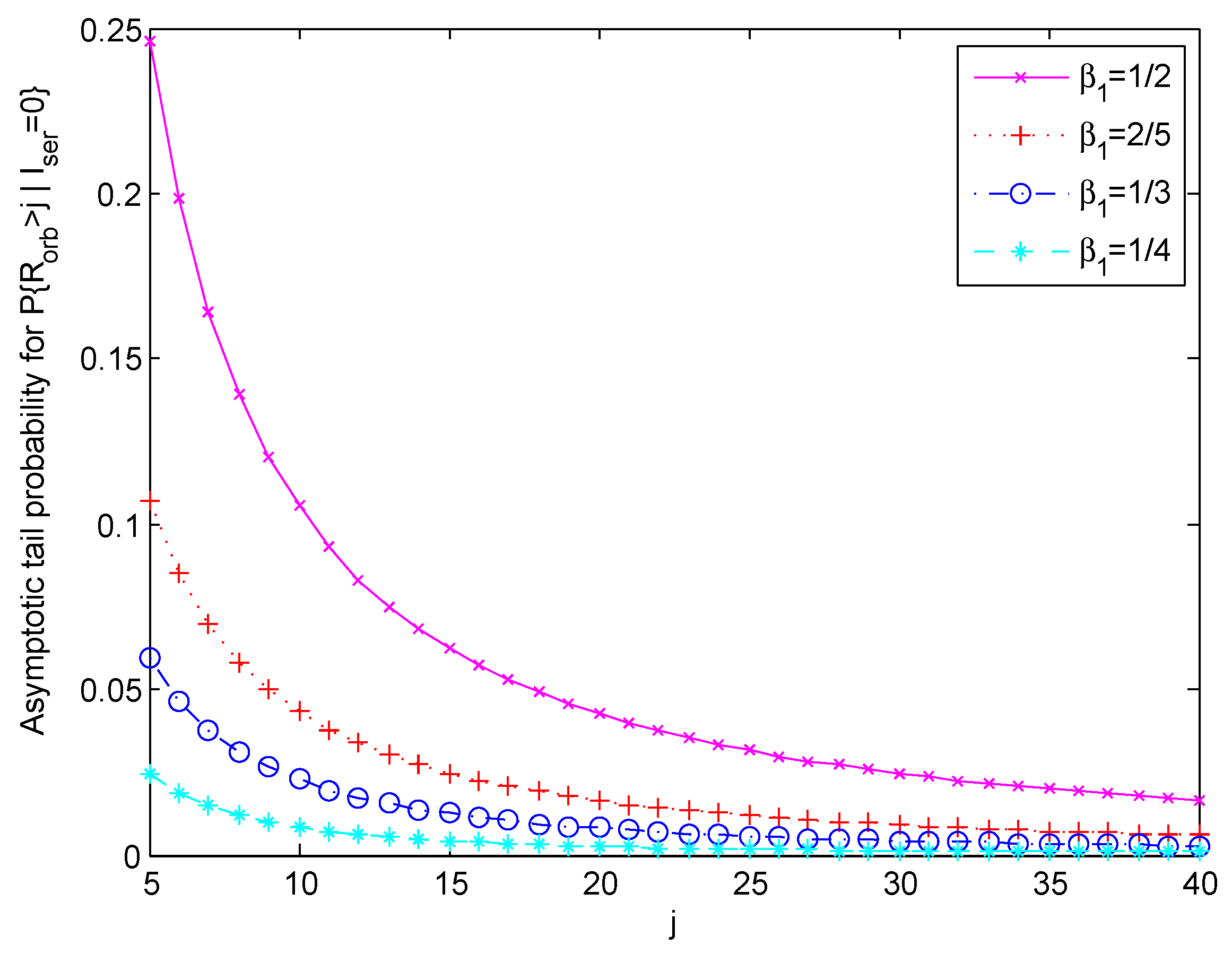
In this section, using numerical examples, we demonstrate how system parameters, like the arrival, service and retrial rates, impact the tail decay rate. According to the tail asymptotic expressions obtained in (30), (39) and (45), it is expected that the tail becomes fatter (or the tail probability becomes bigger) as the arrival rate ($\lambda$) increases while all other parameter values remain the same for all three types of conditional probabilities. Similar results are expected as the service rate (${\beta }_1^{-1}$) or the retrial rate ($\mu$) decreases, respectively. The above claim has been supported by our extensive numerical tests using various slowly varying functions and a broad range of parameter values. For a quantitative pictorial example, we take the conditional tail probability $P\{R_{orb}>j\mid I_{ser}=0\}$ as expressed in (30).

Assume that the service time $T_{\beta }$ follows a Pareto distribution with shape parameter $a>1$ and scale parameter $b>0$, i.e.,

$$F_{\beta }\left(x\right)=1-{\left(1+x/b\right)}^{-a},\mathrm{for}x\ge 0,$$

(46)

for convenience, since, in this case, we can easily compute the mean service time, given as ${\beta }_1=E\left(T_{\beta }\right)=b/(a-1)$ and the traffic intensity, given as $\rho =\lambda {\beta }_1=\lambda b/(a-1)$.

We provide three figures to demonstrate the quantitative changes of the tail probability as a function of the arrival rate $\lambda$, the expected service time ${\beta }_1$, and the retrial rate $\mu$, respectively. In Figure 1, set $a=3/2$, $b=1/5$, $q=1/2$ (Bernoulli probability of joining the queue), and $\mu =1$. Then, the tail asymptotic probability is a function of the arrival rate $\lambda$. Four curves in different colours are given to show the changes as $\lambda$ changes, corresponding to $\lambda =3/4,1,5/4,3/2$, respectively.

In Figure 2, we set $\lambda =1.2$, $q=1/2$ and $\mu =1$. Then, the tail asymptotic probability is a function of the expected service time ${\beta }_1$. By further assuming $b=1/5$, the tail asymptotic probability is simply a function of a (see Assumption 1). In order to see the impact of the service time distribution $F_{\beta }\left(x\right)$ on the asymptotic tail $P\{R_{orb}>j\mid I_{ser}=0\}$, four curves in different colours are given, corresponding to ${\beta }_1=1/2,2/5,1/3,1/4$, respectively (or, correspondingly, $a=1+b/{\beta }_1=1.4,1.5,1.6,1.8$).

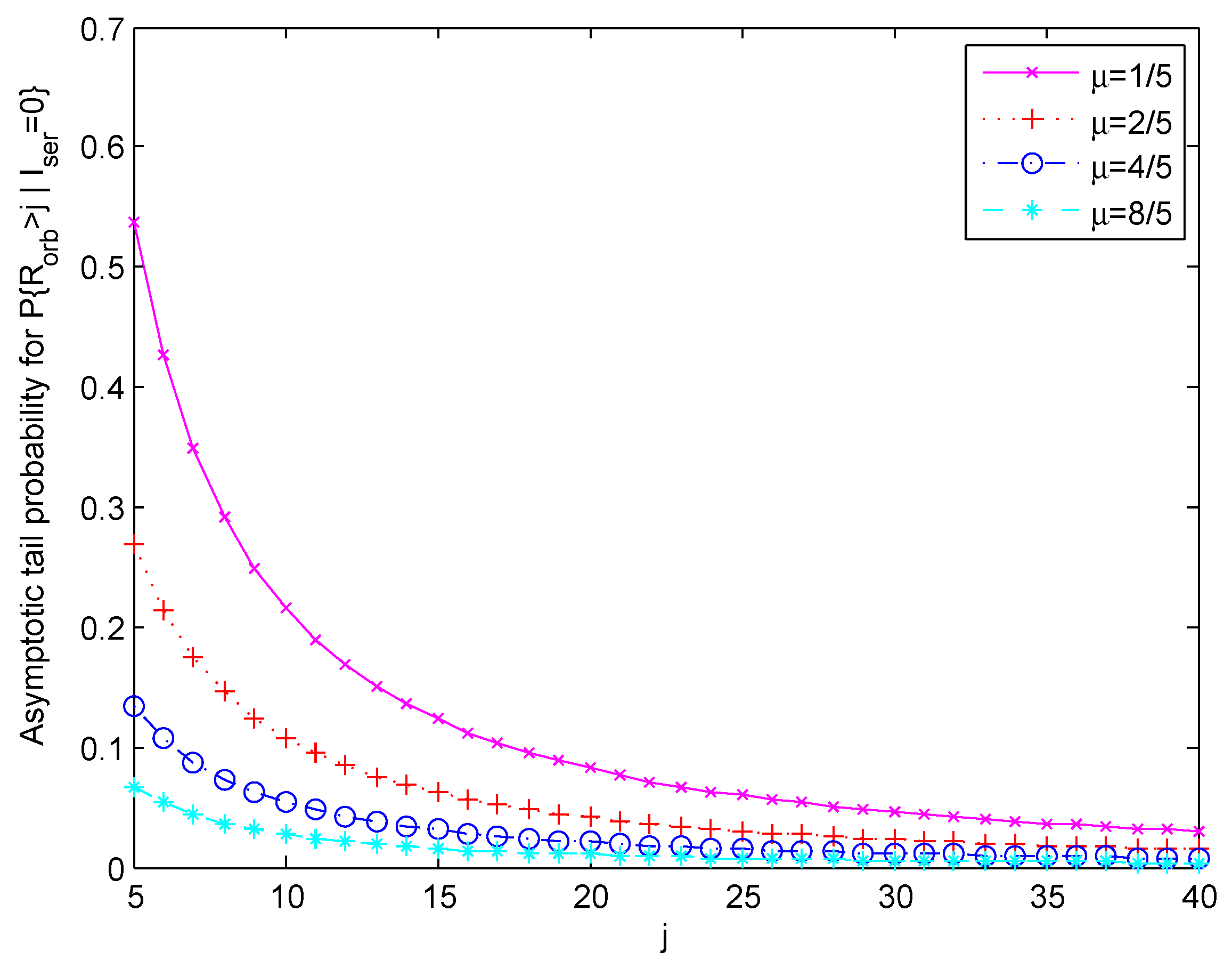
Finally, we show, in Figure 3, the trend of the change for the tail asymptotic probability $P\{R_{orb}>j\mid I_{ser}=0\}$, as a function of the retrial rate $\mu$. Specifically, we set $a=3/2$, $b=1/5$, $\lambda =1.2$ and $q=1/2$. The four curves correspond to the following four different retrial rates: $\mu =1/5,2/5,4/5,8/5$, respectively.

6. Conclusions

In this paper, the exhaustive version of the stochastic decomposition method was used to decompose the generating function $R_0\left(z_2\right)$ (or corresponding r.v. $R_0$) into detailed components, each of which has probabilistic interpretations (see Remark 5). This decomposition leads to a tail asymptotic expression for $P\{R_{orb}>j\mid I_{ser}=0\}$, given in (30). By applying the same decomposition method to the generating function $E\left(z_1^{R_{11}}\right)$ (see Equation (31) and Remark 7), we obtained the tail asymptotic expression for $P\{R_{que}>j\mid I_{ser}=1\}$ given in (39), and by applying the exhaustive version of decompositions to the generating function $E\left(z_2^{R_{12}}\right)$ (see Equation (40) and Remark 8), we obtained the tail asymptotic expression for $P\{R_{orb}>j\mid I_{ser}=1\}$ given in (45).

This exhaustive version of the stochastic decomposition method has also been applied to a priority queueing system in [17] and a retrial queue with batch arrivals in [16]. We expect that the same method can be applied to many other queueing models.