Updating the Landweber Iteration Method for Solving Inverse Problems

Abstract

The Landweber iteration method is one of the most popular methods for the solution of linear discrete ill-posed problems. The diversity of physical problems and the diversity of operators that result from them leads us to think about updating the main methods and algorithms to achieve the best results. We considered in this work the linear operator equation and the use of a new version of the Landweber iterative method as an iterative solver. The main goal of updating the Landweber iteration method is to make the iteration process fast and more accurate. We used a polar decomposition to achieve a symmetric positive definite operator instead of an identity operator in the classical Landweber method. We carried out the convergence and other necessary analyses to prove the usability of the new iteration method. The residual method was used as an analysis method to rate the convergence of the iteration. The modified iterative method was compared to the classical Landweber method. A numerical experiment illustrates the effectiveness of this method by applying it to solve the inverse boundary value problem of the heat equation (IBVP).

1. Introduction

In the early twentieth century, Hadamard [1] labeled the situations for well-posed problems for linear operator equations, stating that a problem is well-posed when it fulfilled the following points:

• Solution exists;
• Uniqueness, this solution is unique;
• Stability (the given data are continuously dependent on the solution).

If at least one of the above points or conditions is not fulfilled in the problem, the problem is considered to be an ill-posed problem. The violations of 1 and 2 can often be improved with a small re-formulation of the problem. Violations of stability are much harder to remedy because they imply that a small disturbance in the data leads to a large disturbance in the estimated solution [2,3,4,5]. The inverse problem under the study of the heat equation can be solved by many methods; for example, the method of regularization by Tikhonov A.N. [6], the method of Lavrentiev M.M. [7], the method of quasi-solutions by Ivanova V.K. [8], and many others.

The Landweber iteration is a basic and initial method for solving inverse problems or linear operator equations. Due to its ease of operation and relatively low complexity per iteration, the Landweber method attracted a lot of attention for studying inverse problems. The useful methods for solving inverse problems depend on the profound insight through the problems related to the algorithms for solving these problems [9,10,11,12,13,14].

Regarding Landweber iterations in Hilbert spaces, see [15,16]. In the last years, the Landweber method has been extended to solve inverse problems in many spaces, such as t Banach spaces [17,18,19]. Many works have modified the Landweber iteration method, such as [20], which used a revision of the residual principle method for iteration of the Landweber in order to solve the inverse problems (linear and non-linear) in Banach spaces and the author proved the new convergence results. In [21], the author estimated the convergence of the error between the exact and estimated solution by considering the regularization level in the estimated solution by using the initial data for selecting the parameter of regularization. In [22], the author presents the Landweber iterative method and accelerates it by using a sparse Jacobian-based reconstruction method.

This article presents an update of the classical Landweber iteration. We use a new reversible operator to increase iteration convergence. We also compared the proposed iterative method with the classical Landweber iteration. A numerical experiment illustrates the effectiveness of this method through an application solving the heat equation’s inverse boundary value problem.

2. Problem Statement

In general, the generic form used to explain numerical solutions to ill-posed problems is applied to the following linear operator equation for the first kind:

$$Au=f,$$

(1)

where $A$ is a linear positive compact operator and act from a Hilbert space $H$ to the same $H$. We also assume that $u,f\in H$ and the operator compressed, self-adjoint, and affirmative description $A:H\to H$. In particular, the operator $A$ is severely ill-conditioned and may be rank-deficient. Operators of this kind arise from the discretization of linear ill-posed problems, such as Fredholm or Volterra integral equations of the first kind.

Right-hand side data are given with some error or measurement noise, which is typical of practical studies. Considering the following scenario to depict this general situation: assume the right-hand side of the problem (1) given with some error level $\delta$. Instead of $f$, we have $f_{\delta }$ with the following norm equation:

$$\Vert f_{\delta }-f\Vert \le \delta ,$$

(2)

We pose a problem that requires finding the estimated solution for (1) and (2) with some input data or information provided in the right-hand side $f_{\delta }$. We called $u_{\alpha }$ an estimated solution, and the parameter $\alpha$ presented the regularization parameter and this parameter linked to the error level $\delta$, i.e., $\alpha =\alpha (\delta )$, and we calculated the error estimate $\Vert u_{\delta }-u\Vert$.

The definition of steady ways for addressing the ill-posed problems are dependent on the usage of a priori data concerning the inexactness of the incoming data. Once the right-hand side is given with some error, we now attempt to solve following problem:

$$A{u}_{\alpha }=f_{\delta },$$

(3)

Variational methods, as an alternative way of solving the problem (3), compute minimizing the norm for the residual form $r=A{u}_{\alpha }-f_{\delta }$, or the functional discrepancy method as the following form:

$$J_0(u_{\alpha })={\Vert A{u}_{\alpha }-f_{\delta }\Vert }^2.$$

(4)

There are varieties of possible solutions to the problem that satisfy Equation (3), which are exact in the face of some discrepancy $\delta$. Considering the well-posed problems required the identification of the class of wanted solutions and clearly giving a priori restrictions on the solution. We are attentive to the bounded solutions for the given problem (1) and (2), hence, the a priori is constrained with the following equation:

$$\Vert u\Vert \le M,$$

(5)

where $M=const>0.$

3. Method of Iterative Regularization

In order to solve the problems with ill-posed definitions, the iteration methods have been successfully used. By calling the problem (1), we will discuss the specific features in of the updated iteration Landweber method below. The ill-posedness behaviors of the inverse problems are connected to the fact that the eigenvalues of operator $A$, shown in reducing order $\left({\lambda }_1\ge {\lambda }_2\ge \dots \ge {\lambda }_k\ge \dots \ge 0\right)$, tend to zero for $k\to \infty$.

The general form of the iteration method for solving Equation (3)with approximately given input data, can be rewritten as following form:

$$u^{k+1}=u^k+{\alpha }_k{A}^{T}E(f_{\delta }-A{u}^k)$$

(6)

in this method, called the two-layer iteration method, the ${\alpha }_k$ is defined as a relaxation parameter and $E$ is a positive definite operator. $E$ is equivalent to the identity operator, the (6) classical Landweber iteration method [23].

There are several well-known methods that can be driven in the form of (3) by selecting the operator $E$. Cimmino’s method [24] is $E=\frac{1}{m}diag\left({1/\Vert a_i\Vert }^2\right)$, where $a_i$ represents the ith row of $A$. The CAV method [25] used the following form of operator $E$ $E=diag\left(1/{\displaystyle \sum _{j=1}^n{N}_j{a}_{ij}^2}\right)$, where $N_j$ is the number of non-zeroes in the jth column of $A$. We define the new type of the Landweber iteration method by using $E$ as follows:

$$E=Q=A{P}^{-1}$$

(7)

Q is unitary operator and $P=\sqrt{A{A}^T}$, by using the polar decomposition of the operator $A$:

$$A=QP,$$

(8)

Now the new version of the iteration method is shown in the following iterative equation:

$$u^{k+1}=u^k+{\alpha }_{k}A{Q}^T(f_{\delta }-A{u}^k)$$

(9)

Depending on the specific method, iteration method (9) can resolve the variational problem by the minimization action of the functional discrepancy method $J_0(u_{\alpha })={\Vert A{u}_{\alpha }-f_{\delta }\Vert }^2.$ We defined the MLI algorithm (Algorithm 1), which represented the Modified-Landweber iterative (MLI).

Algorithm 1 MLI (number iteration)

$u^0=\overline{0},zerosvector.$ $[U,\sum ,V]=SVD(A)$ $Q=U{V}^T$ $u^k=u^0$ $fork=1,2,3,\dots ,\mathrm{iteration}\mathrm{times}$ $u^k=u^k+\alpha A{Q}^T(f_{\delta }-A{u}^k)$ $variational={\Vert A{u}^k-f_{\delta }\Vert }^2$ End loop

The classical Landweber method can be defined by the following algorithm (Algorithm 2), and we called it the Classical-Landweber iterative (CLI) method.

Algorithm 2 CLI (number of iteration)

$u^0=\overline{0},zerosvector.$ $u^k=u^0$ $fork=1,2,3,\dots iterationtimes$ $u^k=u^k+\alpha A^T(f_{\delta }-A{u}^k)$ $variational={\Vert A{u}^k-f_{\delta }\Vert }^2$ End loop

In order to make the iteration method in (9) effective, it is critical to invent faithful stopping criteria. This method consists of reducing the given problem to the variational problem:

$${\Vert A{u}_{n(\delta )}-f_{\delta }\Vert }^2\le {\delta }^2.$$

(10)

The iterating process is much longer with the noise input data $f_{\delta }$, which leads to an iterative solution with a loss of resolution $u^k$. This phenomenon is called semi-convergence and is presented by Natterer [26].

4. Analysis of Convergence of Iterations

In this section, we consider Theorem 1 in [27]. To understand the convergence behavior of the iteration technique, we took a closer look at the errors between the estimated and exact solutions by using the constant parameter ${\alpha }_k=\alpha$.

We called $u^{*}$ as the unique solution for Equation (4).

Theorem 1.

Let ${\alpha }_k=\alpha$for $k\ge 0$. Then, the iterates of (9) converge to a solution (called$u_{\alpha }$) of (4) if and only if $0<\alpha <2/{\sigma }_1^2$ with ${\sigma }_1$ the largest singular value of $\sqrt{Q^T}A$.

Proof of Theorem 1.

Assume $u^0=0$. Let $B=A{Q}^{T}A$ and $c=A{Q}^T{f}_{\delta }$.

Then using (9), we obtain:

$$\begin{array}{l}{u}^k=(I-\alpha B)u^{k-1}+\alpha c=\\ =\alpha {\displaystyle \sum _{j=0}^{k-1}{(I-\alpha B)}^{k-j-1}c}.\end{array}$$

We assume that the singular value decomposition (SVD) for $\sqrt{Q^T}A=U\sum V^T$. We represent $B$ in the following form:

$$B={\left(\sqrt{Q^T}A\right)}^T\left(\sqrt{Q^T}A\right)=V{\sum }^T\sum V^T,$$

(11)

where ${\sum }^T\sum =diag({\sigma }_1^2,{\sigma }_2^2,\dots ,{\sigma }_p^2,0\dots ,0)$, ${\sigma }_1\ge {\sigma }_2\ge \dots \ge {\sigma }_p\ge 0$, and $p=rank(A).$

Using (11), we have

$${\displaystyle \sum _{j=0}^{k-1}{(I-\alpha B)}^{k-j-1}}=V{E}_k{V}^T,$$

(12)

where

$$E_k=diag\left(\frac{1-{(1-\alpha {\sigma }_1^2)}^k}{\alpha {\sigma }_1^2},\dots ,\frac{1-{(1-\alpha {\sigma }_p^2)}^k}{\alpha {\sigma }_p^2},k,\dots k\right).$$

(13)

It follows that:

$$u^k=V(\alpha E_k)V^{T}c=V(\alpha E_k){\sum }^T{U}^T\sqrt{Q^T}{f}_{\delta }={\displaystyle \sum _i^p\{1-{(1-\alpha {\sigma }_i^2)}^k\}}\frac{u_i^T\sqrt{Q^T}{f}_{\delta }}{{\sigma }_i}{v}_i.$$

(14)

with SVD

$$u^{*}=V\overline{E}{U}^T\sqrt{Q^T}{f}_{\delta },$$

(15)

where

$$\overline{E}=diag\left(\frac{1}{{\sigma }_1},\dots ,\frac{1}{{\sigma }_p},0,\dots ,0\right).$$

(16)

Note that if $\left|1-\alpha {\sigma }_i^2\right|<1$, if $\left|1-\alpha {\sigma }_i\right|<1$, for $i=1,2,\dots ,p$, i.e., $0<\alpha <\frac{2}{{\sigma }_1^2}$, we find

$$\underset{k\to \infty }{\lim }\left(\alpha E_k{\sum }^T\right)=\overline{E}.$$

This completes the proof. □

5. Number of Iterations

We need to formulate the conditions under which MLI (9) provides the estimated solution for problem (1) and (2) after the number of iterations $n(\delta )$.

Theorem 2.

Let the number of iterations in MLI (9) $n(\delta )\to \infty$and$n(\delta )\delta \to 0$as$\delta \to 0$. Then,$\Vert u_{n(\delta )}-u\Vert \to 0$such that$\delta \to 0$.

Proof of Theorem 2.

We represent the inexactness at the nth iteration as $z_n=u_n-u$. By (9), we obtain:

$$u^n={\left(I-\alpha A{Q}^T\right)}^n{u}^0+{\displaystyle \sum _{k=0}^{n-1}{\left(I-\alpha A{Q}^T\right)}^k\alpha f_{\delta }}.$$

(17)

where $u^0$ some initial estimate.

In order to find the exact solution, we can use the following representation:

$$u={\left(I-\alpha A{Q}^T\right)}^{n}u+{\displaystyle \sum _{k=0}^{n-1}{\left(I-\alpha A{Q}^T\right)}^k\alpha f}.$$

This illustration corresponds to the iteration solution for problem (1) in which the initial approximation coincides with the exact solution.

With equality (17) taken into account, for the inexactness, we obtain the following:

$$z_n=z_n^{(1)}+z_n^{(2)}$$

(18)

where $z_n^{(1)}={\left(I-\alpha A{Q}^T\right)}^n{z}^0,z_n^{(2)}={\displaystyle \sum _{k=0}^{n-1}{\left(I-\alpha A{Q}^T\right)}^k\alpha \left(f_{\delta }-f\right)}$, with $z^0=u^0-u$ being inexactness. The first term $z_n^{(1)}$ in (18) is in the iteration method, and the term $z_n^{(2)}$ is related to the inexactness on the input data of (1).

Under $0<\alpha <\frac{2}{\gamma }$, where $\gamma >0$, we take

$$\Vert I-\alpha A{Q}^T\Vert \le 1.$$

(19)

In order to verify this variation, we have passed from difference (19) to the equivalent inequality

$$\left(I-\epsilon Q{A}^T\right)\left(I-\alpha A{Q}^T\right)\le I$$

where $A$ self-adjoint and positive definition with the estimate $A{Q}^T>\gamma I$ taken into account, we obtain:

$$\begin{array}{l}\left(I-\alpha Q{A}^T\right)\left(I-\alpha A{Q}^T\right)-I=\\ =\alpha \sqrt{A{Q}^T}\left(\alpha A{Q}^T-2I\right)\sqrt{A{Q}^T}\le \alpha \sqrt{A{Q}^T}\left(\alpha \gamma -2\right)\sqrt{A{Q}^T}\le 0.\end{array}$$

provided $0<\alpha <\frac{2}{\gamma }$ is satisfied.

Taking inequality (19), we obtained:

$$z_n^{(2)}={\displaystyle \sum _{k=0}^{n-1}{\Vert I-\alpha A{Q}^T\Vert }^k\alpha \Vert f_{\delta }-f\Vert }\le n\alpha \delta .$$

(20)

The estimate $z_n^{(1)}$ deserves a more detailed study. To begin with, assume that $z^0\in H$. Such a situation is met, for instance, with the initial approximation $u^0=0$ in the solution to problems (1) and (2) in class (5). Let us show that $s(n)=\Vert z_n^{(1)}\Vert \to 0$ for $n\to \infty$. We use the representation:

$$s^2(n)={\displaystyle \sum _{i=1}^{\infty }{\left(1-\alpha {\sigma }_i\right)}^{2n}{\left(z^0,w_i\right)}^2.}$$

For any small $\epsilon >0$, can found N such that

$${\displaystyle \sum _{i=N+1}^{\infty }{\left(z^0,w_i\right)}^2\le \frac{\epsilon }{2}.}$$

By $\left|1-\alpha {\sigma }_i\right|<1$, we obtain:

$$s^2(n)\le {\displaystyle \sum _{i=1}^N{\left(1-\alpha {\sigma }_i\right)}^{2n}{\left(z^0,w_i\right)}^2+{\displaystyle \sum _{i=N+1}^{\infty }{\left(z^0,w_i\right)}^2.}}$$

In case of sufficiently large N, for the first term we obtain the following:

$${\displaystyle \sum _{i=1}^N{\left(1-\alpha {\sigma }_i\right)}^{2n}{\left(z^0,w_i\right)}^2}\le \frac{\epsilon }{2}.$$

The substitution of (20) into (18) yields the estimate

$$\Vert z_n\Vert \le n\alpha \delta +s(n).$$

(21)

such that $s(n)\to 0$ for $n\to \infty$. Estimating (21) completes the proof. □

In the updated iteration method (9), the number of iterations matched the inexactness input data; also the input data or right-hand side serves the regularization parameter.

6. Estimating the Rate of Convergence

We know the convergence without needing the discovery the rate. By narrowing the class of a priori limitations of the solution, we define the following theorem for the estimated solution as an explicit function of the inexactness of the input data.

Consider the iterative method (9) under the more stringent constraints of the iterative parameter,

$$0<\alpha <2/{\sigma }_1^2,$$

(22)

Theorem 3.

Suppose that the exact solution of problem (3) belongs to the class

$$\Vert A^{-p}u\Vert \le M,0<p<\infty .$$

(23)

 Then, for the inaccuracy of the iteration method (9) with  $u_0=0$ their holds the estimate

$$\Vert z_n\Vert \le n\alpha \delta +M_1{n}^{-p},M_1=M_1(\alpha ,p,M).$$

(24)

Proof of Theorem 3.

By condition (23), it is necessary to know the quantity of $s(n)$ in (21). The iterations number n determines the outcome.

With $u^0=0$, we find $z^0=u$, by using the above, we find:

$$z_n^{(1)}={\displaystyle \sum _{i=1}^{\infty }{\sigma }_i^p{(1-\alpha {\sigma }_i)}^n\frac{\left(u,w_i\right)}{{\sigma }_i^p}{w}_i.}$$

After that, in view of (23) we find:

$$s(n)\le \underset{{\sigma }_i}{\max }{\displaystyle \sum _{i=1}^{\infty }{\sigma }_i^p{\left|1-\alpha {\sigma }_i\right|}^n\Vert A^{-p}u\Vert .}$$

(25)

Under constraint (22) on the iteration parameter, we have $o<\alpha {\sigma }_i\le 1$ and, hence,

$$s(n)\le \underset{{\sigma }_i}{\max }{\sigma }_i^p{\left|1-\alpha {\sigma }_i\right|}^n\le \frac{1}{{\alpha }^p}\underset{0<\eta <1}{\max }\chi (\eta ),$$

where $\chi (\eta )={\eta }^p{(1-\eta )}^n$. The function $\chi (\eta )$ attains its maximum at the point

$$\eta ={\eta }^{*}=\frac{p}{p+n}$$

and,

$$\chi ({\eta }^{*})={\left(\frac{p}{n}\right)}^p{\left(1-\frac{p}{p+n}\right)}^{p+n}<\frac{p^p}{n^p}\exp (-p).$$

Replace the (25) solutions in estimate (24), in which the constant

$$M_1=\frac{p^p}{{\alpha }^p}\exp (-p)M$$

depends on $p,\alpha$ and $M$, and does not depend on $n$. Minimizing the input data of (24) lets us formulate the stop criterion:

$$n_{opt}={\left(\frac{p{M}_1}{\alpha }\right)}^{1/(p+1)}{\delta }^{-1/(p+1)},$$

(26)

i.e., $n(\delta )=\vartheta ({\delta }^{-1/(p+1)})$. Here, for the inexactness of the estimated solution, we obtain the following estimation

$$\Vert z_{n_{opt}}\Vert \le M_2{\delta }^{p/(p+1)}$$

(27)

with

$$M_2=\alpha {\left(\frac{p{M}_1}{\alpha }\right)}^{1/(p+1)}+M_1{\left(\frac{p{M}_1}{\alpha }\right)}^{-p/(p+1)}.$$

The approximation of (27) establishes the direct requirement of the rate at which the approximated solution converges to the exact solution on inexactness δ and on the exact solution’s smoothness (parameter p). □

7. Numerical Results

We considered the inverse boundary value problem found in [28]:

$$\frac{\partial u\left(x,t\right)}{\partial t}=\frac{{\partial }^{2}u\left(x,t\right)}{\partial x^2};0<x<1,0<t\le T,$$

(28)

$$u\left(x,0\right)=0;0\le x\le 1,$$

(29)

$$\frac{\partial u\left(0,t\right)}{\partial x}=0;0<t\le T,$$

(30)

$$u\left(1,t\right)=u\left(t\right);0<t\le T,$$

(31)

supposing that the $u\left(t\right)$ is a function such that

$$u\left(t\right)\in H^4\left[0,T\right],u\left(0\right)=u^{\prime }\left(0\right)=u^{″}\left(0\right)=u^{″}\left(T\right)=u^{″}\left(T\right)=0,$$

(32)

and $\underset{0}{\overset{T}{{\displaystyle \int }}}{\left|u^{‴}\left(t\right)\right|}^{2}dt\le r^2,$ $r$ is the identified number. By applying the separation of variables method, we achieve:

$$u\left(x_0,t\right)={\displaystyle \sum }_{n=0}^{\infty }{a}_n\left(t\right)\mathrm{c}\mathrm{o}\mathrm{s}((n+0.5)\pi x_0)+u\left(t\right),$$

(33)

where $x_0\in \left(0,1\right),t\in \left[0,T\right]$ and

$$a_n\left(t\right)=\frac{2e^{-{\left(n+0.5\right)}^2{\pi }^{2}t}}{\left(n+0.5\right)\pi }\underset{0}{\overset{t}{{\displaystyle \int }}}{h}^{\prime }\left(\tau \right)e^{{\left(n+0.5\right)}^2{\pi }^2\tau }d\tau ,$$

(34)

Integrating by two parts for the right-hand side of (34), we obtain:

$$\begin{array}{c}{a}_n\left(t\right)=\frac{2}{\left(n+0.5\right)\pi }\underset{0}{\overset{t}{{\displaystyle \int }}}{u}^{‴}\left(\tau \right)e^{-{\left(n+0.5\right)}^2{\pi }^2\left(t-\tau \right)}d\tau +\frac{2}{{\left(n+0.5\right)}^3{\pi }^3}{u}^{\prime }\left(t\right)\\ -\left[\frac{2}{{\left(n+0.5\right)}^3{\pi }^3}{u}^{\prime }\left(0\right)+\frac{2}{{\left(n+0.5\right)}^5{\pi }^5}{u}^{″}\left(t\right)+\frac{2}{{\left(n+0.5\right)}^5{\pi }^5}{u}^{″}\left(0\right)\right]\end{array},$$

(35)

$$\begin{array}{c}{a}_n\left(t\right)=\frac{2}{{\left(n+0.5\right)}^5{\pi }^5}\underset{0}{\overset{t}{{\displaystyle \int }}}{u}^{‴}\left(\tau \right)e^{-{\left(n+0.5\right)}^2{\pi }^2\left(t-\tau \right)}d\tau \\ -\left[\frac{2}{{\left(n+0.5\right)}^3{\pi }^3}{u}^{\prime }\left(0\right)+\frac{2}{{\left(n+0.5\right)}^5{\pi }^5}{u}^{″}\left(0\right)\right]\end{array},$$

(36)

where $u^{\prime }\left(0\right)=u^{″}\left(0\right)=0$, by (32) and

$$a_n\left(t\right)=\frac{2}{{\left(n+0.5\right)}^5{\pi }^5}\underset{0}{\overset{t}{{\displaystyle \int }}}{u}^{‴}\left(\tau \right)e^{-{\left(n+0.5\right)}^2{\pi }^2\left(t-\tau \right)}d\tau ,$$

(37)

From (33) and (37) we find the next integral equation for the first kind:

$$f\left(t\right)=u\left(x_0,t\right)=u\left(t\right)+\underset{0}{\overset{t}{{\displaystyle \int }}}{\displaystyle \sum }_{n=0}^{\infty }\frac{2\mathrm{c}\mathrm{o}\mathrm{s}\left(n+0.5\right)\pi x_0}{{\left(n+0.5\right)}^5{\pi }^5}{e}^{-{\left(n+0.5\right)}^2{\pi }^2\left(t-\tau \right)}g(\tau )d\tau ,$$

(38)

where $u^{‴}\left(\tau \right)=g(\tau )$. We define the operator $P: L_2\left[a, b\right] \to L_2\left[a, b\right]$ by:

$$u\left(t\right)=Pg\left(\tau \right)=\underset{0}{\overset{t}{{\displaystyle \int }}}\frac{{\left(t-\tau \right)}^2}{2}g\left(\tau \right)d\tau ,g\left(\tau \right),Pg\left(\tau \right)\in L_2\left[0,T\right],$$

(39)

We used the discretization algorithm in [29] and applied it in [30], by specifying the derivative for the kernel we achieve the following:

$$Au\left(t\right)=\underset{0}{\overset{t}{{\displaystyle \int }}}K\left(t,\tau \right)g\left(\tau \right)d\tau =f\left(t\right), t\in \left[0,T\right],$$

(40)

where $K(t,\tau )=\frac{{(t-\tau )}^2}{2}+{\displaystyle \sum _{n=0}^{\infty }\frac{2cos(n+0.5)\pi x_0}{{(n+0.5)}^5{\pi }^5}{e}^{-{\left(n+0.5\right)}^2{\pi }^2\left(t-\tau \right)}}$.

The operator $A$ is an infinite-dimensional operator. The next step applies the discretization algorithm to the integral Equation (40) and converts the operator $A$ to the finite-dimension operator $A_n$, where $A_n\to A$ for $n\to \infty ,$ and for operator $P$, there is an operator $P_n$, where $P_n\to P$ for $n\to \infty ,$

$${\overline{K}}_i\left(t\right)=K\left({\tau }_i,t\right),$$

(41)

$${\overline{K}}_i\left(t\right);{\tau }_i\le \tau \le {\tau }_{i+1},t\in \left[0,T\right],i=0,1, \dots ,n-1,$$

(42)

$${\overline{K}}_i\left(t_j\right);{\tau }_i\le \tau \le {\tau }_{i+1},t_j\le t\le t_{j+1},i=0,1,\dots ,n-1,j=0,1\dots ,n-1,$$

(43)

$$K_n\left(t,\tau \right)={\overline{K}}_i\left(t_j\right),$$

(44)

$$A_n\left[u\left(t\right)\right]=\underset{0}{\overset{t}{{\displaystyle \int }}}{K}_n\left(t,\tau \right)g\left(\tau \right)d\tau =f\left(t\right),t\in \left[0,T\right],$$

(45)

$${\overline{K}}_i\left(t_j\right)=\{\begin{array}{c}K\left({\tau }_i,t_j\right)\hspace{1em}i\le j\\ 0\hspace{1em}\hspace{1em}i>j\end{array}.$$

(46)

From the above, we convert the system of differential Equations (28)–(32) to the linear operator equation $A_{n}u=f_n,$ where $u=P_{n}g,$ by reformulating the differential equation to an integral equation by using the separation of variables and applying the discretization algorithm to convert the integral equation into a system of linear algebra equations or linear operator equations.

$${\overline{A}}_n\left[\begin{array}{c}g\left({\tau }_0\right)\\ g\left({\tau }_1\right)\\ ⋮\\ g\left({\tau }_{n-1}\right)\end{array}\right]=\left[\begin{array}{c}f\left(t_0\right)\\ f\left(t_2\right)\\ ⋮\\ f\left(t_{n-1}\right)\end{array}\right],$$

(47)

where

$${\overline{A}}_n=\frac{1}{n}\left[\begin{array}{cc}\begin{array}{cc}K\left({\tau }_0,t_0\right)& 0\\ K\left({\tau }_0,t_1\right)& K\left({\tau }_1,t_1\right)\end{array}& \begin{array}{cc}\dots & 0\\ \dots & 0\end{array}\\ \begin{array}{cc}⋮& ⋮\\ K\left({\tau }_0,t_{n-1}\right)& K\left({\tau }_1,t_{n-1}\right)\end{array}& \begin{array}{cc}\dots & ⋮\\ \dots & K\left({\tau }_{n-1},t_{n-1}\right)\end{array}\end{array}\right],$$

(48)

where ${\overline{A}}_n=A_n{P}_n$

The operator ${\overline{A}}_n$ in (43) is a non-injective operator, because it has the triangular property [28].

Considering the above problem, we need to find the function $u\left(t\right)\in H^4\left[0,T\right]$. The real solution, and the $u\left(x_0,t\right)=f\left(t\right)$ represented the input function, where the $x_0\in \left(0,1\right),t\in \left[0,T\right]$, $x_0=0.5$ and $T=1$. In [31], we prepared a case study using MATLAB code. First of all, the discretization algorithm was applied to obtain the operator, and by using $u\left(t\right)=\sin (\pi /2\ast t)$, we obtained the vector $f$. We then add some noise, as explained in the code for obtaining the vector $f_{\delta }$. Finally, we computed the SVD for operator $A$, and used it in the MLI and CLI algorithms to obtain the approximation solutions $u_{\alpha }$.

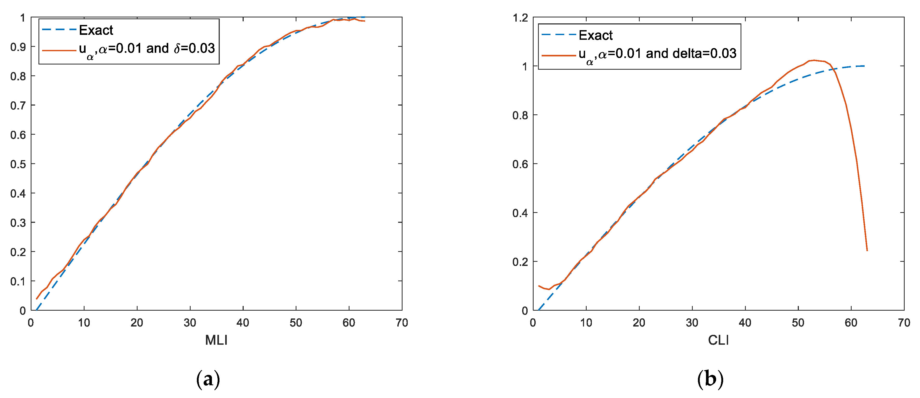
Algorithm 1 MLI (number iteration): MLI the value of the regularization parameter that was used with 1000 iterations (see Figure 1).

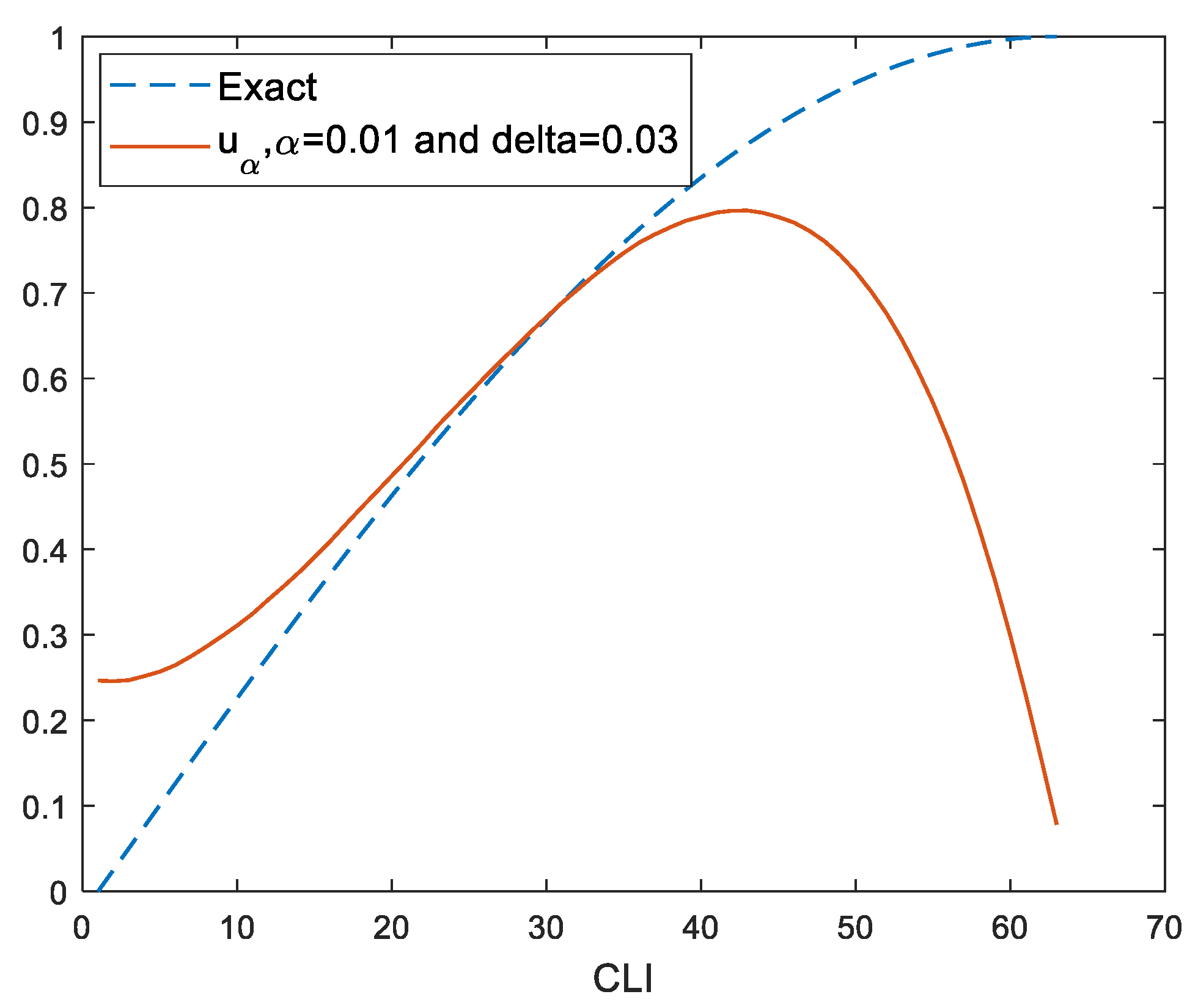
Algorithm 2 CLI (number of iteration): the value of regularization parameter with 1000 iterations (see Figure 2).

In Figure 3, the iterations increased to 10,000.

In Figure 4, the iterations increased to 20,000.

8. Conclusions Remarks and Observations

This paper defined algorithms that solve ill-posed inverse problems by using an iterative regularization method (Landweber iterative type). The regularization parameter was chosen by considering the iteration method that was most consistent with the real solution. The residual method was used as an analysis method to rate the last iteration’s convergence. We observed that the minimum of the discrepancy is extremely unstable with respect to data perturbations on the right-hand side of the linear operator equation. It is clear that the updated Landweber iteration algorithm obtained a good approximation solution compared with the classical Landweber method. That means that our updated Landweber method successfully fixed this instability in the discrepancy method. The suggested algorithms successfully solve the inverse boundary value problem for the heat-conducting problem.

References

- Daniell, P.J.; Hadamard, J. Lectures on Cauchy’s Problem in Linear Partial Differential Equations. Math. Gaz. 1924, 12, 173. [Google Scholar] [CrossRef]
- Al-Mahdawi, H.K. Studying the Picard’s Method for Solving the Inverse Cauchy Problem for Heat Conductivity Equations. Bull. South Ural State Univ. Ser. Comput. Math. Softw. Eng. 2019, 8, 5–14. [Google Scholar] [CrossRef]
- Al-Mahdawi, H.K. Development the Regularization Computing Method for Solving Boundary Value Problem to Heat Equation in the Composite Materials. J. Phys. Conf. Ser. 2021, 1999, 12136. [Google Scholar] [CrossRef]
- Al-Mahdawi, H.K. Development the Numerical Method to Solve the Inverse Initial Value Problem for the Thermal Conductivity Equation of Composite Materials. J. Phys. Conf. Ser. 2021, 1879, 32016. [Google Scholar] [CrossRef]
- Al-Mahdawi, H.K.; Sidikova, A.I. An Approximate Solution of Fredholm Integral Equation Of The First Kind By The Regularization Method With Parallel Computing. Turkish J. Comput. Math. Educ. 2021, 12, 4582–4591. [Google Scholar]
- Tikhonov, A.N. On the Regularization of Ill-Posed Problems. Proc. USSR Acad. Sci. 1963, 153, 49–52. [Google Scholar]
- Lavrentiev, M.M. The Inverse-Problem in Potential Theory. Dokl. Akad. Nauk SSSR 1956, 106, 389–390. [Google Scholar]
- Ivanov, V.K. The application of Picard’s method to the solution of integral equations of the first kind. Bull. Inst. Politenn. Iasi. 1968, 14, 71–78. [Google Scholar]
- Glasko, V.B.; Kulik, N.I.; Shklyarov, I.N.; Tikhonov, A.N. An inverse problem of heat conductivity. Zhurnal Vychislitel’ noi Mat. i Mat. Fiz. 1979, 19, 768–774. [Google Scholar]
- Belonosov, A.S.; Shishlenin, M.A. Continuation problem for the parabolic equation with the data on the part of the boundary. Siber. Electron. Math. Rep. 2014, 11, 22–34. [Google Scholar]
- Kabanikhin, S.I.; Hasanov, A.; Penenko, A.V. A gradient descent method for solving an inverse coefficient heat conduction problem. Numer. Anal. Appl. 2008, 1, 34–45. [Google Scholar] [CrossRef]
- Yagola, A.G.; Stepanova, I.E.; Van, Y.; Titarenko, V.N. Obratnye zadachi i metody ikh resheniya: Prilozheniya k geofizike (Inverse Problems and Methods for Their Solution: Applications to Geophysics); Binom. Laboratoriya Znanii: Moscow, Russia, 2014. [Google Scholar]
- Kabanikhin, S.I.; Krivorot’ko, O.I.; Shishlenin, M.A. A numerical method for solving an inverse thermoacoustic problem. Numer. Anal. Appl. 2013, 6, 34–39. [Google Scholar] [CrossRef]
- Tanana, V.P. On the order-optimality of the projection regularization method in solving inverse problems. Sib. Zhurnal Ind. Mat. 2004, 7, 117–132. [Google Scholar]
- Clason, C.; Nhu, V.H. Bouligand-Levenberg-Marquardt iteration for a non-smooth ill-posed inverse problem. arXiv 2019, arXiv:1902.10596. [Google Scholar] [CrossRef]
- Clason, C.; Nhu, V.H. Bouligand–Landweber iteration for a non-smooth ill-posed problem. Numer. Math. 2019, 142, 789–832. [Google Scholar] [CrossRef] [Green Version]
- Jin, Q. Landweber-Kaczmarz method in Banach spaces with inexact inner solvers. Inverse Probl. 2016, 32, 104005. [Google Scholar] [CrossRef] [Green Version]
- Kaltenbacher, B.; Schöpfer, F.; Schuster, T. Convergence of some iterative methods for the regularization of nonlinear ill-posed problems in Banach spaces. Inverse Probl. 2009, 25, 19. [Google Scholar] [CrossRef] [Green Version]
- Schöpfer, F.; Louis, A.K.; Schuster, T. Nonlinear iterative methods for linear ill-posed problems in Banach spaces. Inverse Probl. 2006, 22, 311. [Google Scholar] [CrossRef] [Green Version]
- Real, R.; Jin, Q. A revisit on Landweber iteration. Inverse Probl. 2020, 36, 75011. [Google Scholar] [CrossRef]
- Li, D.-G.; Fu, J.-L.; Yang, F.; Li, X.-X. Landweber Iterative Regularization Method for Identifying the Initial Value Problem of the Rayleigh–Stokes Equation. Fractal Fract. 2021, 5, 193. [Google Scholar] [CrossRef]
- Wang, J. A two—Step accelerated Landweber—Type iteration regularization algorithm for sparse reconstruction of electrical impedance tomography. Math. Methods Appl. Sci. 2021, 1–12. [Google Scholar] [CrossRef]
- Landweber, L. An Iteration Formula for Fredholm Integral Equations of the First Kind. Am. J. Math. 1951, 73, 615. [Google Scholar] [CrossRef]
- Cimmino, G. Cacolo approssimato per le soluzioni dei systemi di equazioni lineari. La Ric. Sci. 1938, 1, 326–333. [Google Scholar]
- Censor, Y.; Gordon, D.; Gordon, R. Component averaging: An efficient iterative parallel algorithm for large and sparse unstructured problems. Parallel Comput. 2001, 27, 777–808. [Google Scholar] [CrossRef]
- Natterer, F. Computerized tomography. In The Mathematics of Computerized Tomography; Springer: Berlin/Heidelberg, Germany, 1986; pp. 1–8. [Google Scholar]
- Mesgarani, H.; Azari, Y. Numerical investigation of Fredholm integral equation of the first kind with noisy data. Math. Sci. 2019, 13, 267–268. [Google Scholar] [CrossRef] [Green Version]
- Al-Mahdawi, H.K. Solving of an Inverse Boundary Value Problem for the Heat Conduction Equation by Using Lavrentiev Regularization Method. J. Phys. Conf. Ser. 2021, 1715, 12032. [Google Scholar] [CrossRef]
- Tanana, V.P.; Vishnyakov, E.Y.; Sidikova, A.I. An approximate solution of a Fredholm integral equation of the first kind by the residual method. Numer. Anal. Appl. 2016, 9, 74–81. [Google Scholar] [CrossRef]
- Al-Mahdawi, H.K. Development of a numerical method for solving the inverse Cauchy problem for the heat equation. Bull. South Ural State Univ. Ser. Comput. Math. Softw. Eng. 2019, 8, 22–31. [Google Scholar]
- Al-Mahdawi, H.K. BVP_PDE_Heat; GitHub Inc.: San Francisco, CA, USA, 2022; Available online: https://github.com/hssnkd1/BVP_PDE_Heat/blob/main/Landweber (accessed on 25 May 2022).