Abstract
Ground surface roughness is difficult to predict through a physical model due to its complex influencing factors. BP neural networks (BPNNs), a promising method, have been widely applied in the prediction of surface roughness. This paper uses the concept of BPNN to predict ground surface roughness considering the state of the grinding wheel. However, as the number of input parameters increases, the local optimum solution of the model that arises is more serious. Therefore, “identify factors” are designed to judge the iterative state of the model, whilst “memory factors” are designed to store the best weights during network training. The iterative termination conditions of the model are improved, and the learning rate and update rules of the weights are adjusted to avoid the local optimal solution. The results show that the prediction accuracy of the presented model is higher and more stable than the traditional model. Under three types of iteration steps, the average prediction accuracy is improved from 0.071, 0.065, 0.066 to 0.049, 0.042, 0.039 and the standard deviation of prediction decreased from 0.0017, 0.0166, 0.0175 to 0.0017, 0.0070, 0.0076, respectively. Therefore, the proposed method provides guidance for improving the global optimization ability of BPNNs and developing more accurate models for predicting surface roughness.
MSC:
68T07
1. Introduction
Grinding is a widely used practice in precision machining, and the grinding quality directly affects the surface finish and working life of products. Surface roughness is an important parameter for evaluating the quality of ground surfaces and the competitiveness of the overall grinding system, which is closely related to the assembly accuracy, corrosion resistance and wear resistance of the products [1]. Predicting the surface roughness accurately for the grinding process is beneficial for selecting efficient process parameters and guaranteeing the grinding quality. Hence, high-precision prediction of ground surface roughness is of great importance [2,3].
In the research of grinding mechanisms, most physical models only consider the grinding wheel speed, workpiece speed, and depth of cut. However, surface roughness is equally sensitive to wheel wear, and it is difficult for the physical model to consider the time-varying state of the grinding wheel. Statistical analysis is commonly used for prediction [4,5], but it has limitations in solving complex nonlinear relationships such as grinding processes. Therefore, to meet the control needs of actual processing, researchers are more inclined to use machine learning models to predict surface roughness [6,7,8,9,10]. Nikolaos et al. [11] took the depth of cut, feed rate, and spindle speed as input parameters to establish an artificial neural network to predict the ground surface roughness Ra. The results showed that the prediction accuracy was as high as 0.796, which proved the validity of the model. To control the surface roughness during high-speed machining, Jiao et al. [12] used a fuzzy adaptive network to predict the surface roughness. The results showed that the average absolute error of the model was 0.25 μm, while that of the regression analysis method was 0.70 μm. Kechagias et al. [13] took the upper width, down width, and kerf angle as input parameters to establish a feed-forward and backpropagation neural network to predict the ground surface roughness Ra. The results showed that the complex correlation coefficients between the predicted and experimental values of surface roughness were all greater than 0.975, which proved the model validity. As a typical machine learning algorithm, BP neural networks (BPNNs) are widely used in the development of surface roughness prediction models due to their strong self-learning ability, high fault tolerance, and circumvention of the revelation of complex physical mechanisms. Baseri et al. [14] took the depth of cut, feed rate, and grinding wheel speed as input parameters to establish a BPNN to predict the ground surface roughness and verify the efficiency of the model. To reduce the effect of tool chatter on the workpiece surface of metal cutting, Shrivastava et al. [15] used an artificial neural network and multi-objective genetic algorithm to predict the optimal cutting zone. The results showed that the tool chatter was most closely related to the depth of cut compared to the feed rate and cutting speed. According to the interaction mechanism between abrasive grains and workpiece in the grinding area, Jiang et al. [16] established a prediction model for the ground surface roughness. The results showed that under the basic parameters of depth of cut, feed rate, and grinding wheel speed, the prediction error decreased from 50% to 10% when the grinding wheel wear was considered. At present, the wear of the grinding wheel is generally studied through force signal. Zhou et al. [17] collected the cutting force signals and extracted features such as average force value, standard deviation, and frequency domain energy with a force sensor. The tool wear was predicted based on the SVD linear feature recognition method, followed by verifying the feasibility of the method through experiments. Elbestawima et al. [18] extracted the components of the milling force signal in each direction and the harmonic power to identify the tool wear, and the results showed that the accuracy rate was between 85% and 100%.
Based on neural networks and physical models, the above studies have developed the relationship between surface roughness, force signal, and grinding wheel wear from the perspectives of time domain, frequency domain, and time–frequency domain. However, problems such as slow convergence and local optimal solutions exist in BPNNs and become more serious with the increase of input dimensions. Additionally, these problems lead to the reduction of the efficiency of model prediction, a large fluctuation in accuracy, and deterioration of stability. Therefore, it is necessary to optimize the BPNN. At present, the optimization methods of BPNNs are mainly divided into three types. The first is to optimize the BPNN based on the swarm algorithm [19,20,21,22,23,24,25]. To solve the problem of the BP model easily falling into local optimal solutions, Chu et al. [26] proposed a simplified PSO algorithm based on a stochastic inertia weight algorithm. The results showed that the convergence speed of the model was increased by two times and the prediction accuracy increased from 75% to 85%. The principle of swarm optimization is to generate multiple groups of initial weights of the BPNN for network training, and then select the optimal weights. Because the different initial weights will cause the BPNN to fall into different local optimal solutions. This approach reduces the adverse effects of a single local optimal solution. The second is to optimize the BPNN based on a genetic algorithm [10,27,28,29,30]. Ding et al. [31] used a genetic algorithm with good global search ability to train the network, and then used the BPNN with good local search ability to find the optimal solution. The optimization principle of a genetic algorithm is to generate multiple groups of initial weights of the BPNN, select the optimal solution through the fitness function, and then update the initial weight group for network training. This approach reduces the influence of the local optimal solution by continuously updating the weight group. The third is to adaptively change the learning rate of the BPNN. Liu and Gao et al. [32,33] changed the learning rate of the BPNN through the size of the training function error, which improved the convergence speed of the BPNN and reduced the impact of the local optimal solution. In the above studies, different optimization algorithms were applied to improve the global search ability of the BPNN in the prediction of surface roughness. The first two types of approaches improved the global search ability by expanding the number of weighted solutions, but the model would still fall into the local optimal solution. In addition, the threshold for iteration termination was selected artificially, resulting in over-convergence and non-convergence of the network; they could not achieve fast convergence and local accurate search of the network at the same time or maximize the prediction performance of the model. In the third type of approach, the learning rate could not be adjusted based on the network training state. Adjusting the learning rate too early or too late would reduce the prediction accuracy and make it not possible to effectively solve the local optimal solution problem. Therefore, improving the local optimal solution and convergence of a BPNN while ensuring the convergence efficiency and prediction accuracy is still a problem to be solved.
In this paper, an adaptive BP network for the prediction of ground surface roughness is proposed to settle these matters, processing the force signal and extracting the features of grinding wheel wear as input parameters. In addition, optimizing the BP algorithm, improving the iterative termination conditions of the prediction model, and adjusting the weight update rules help to solve the problem of local optimal solutions and reduce the impact of human factors. Furthermore, dynamically adjusting the learning rate based on the iterative state of the network maximizes the prediction performance of the model itself, and improves the search accuracy of the target weights with the premise of ensuring rapid convergence. The rationality of the method is verified by comparing the prediction performance of the BP model of ground surface roughness before and after optimization.
2. Data Source and Processing
2.1. Experimental Setup
The experimental material was quartz glass, which was cut into standard specimens with a size of 15 mm × 15 mm × 10 mm. To explore the effect of grinding wheel wear on ground surface roughness, the same grinding wheel was used continuously for processing in the experiment. The grinding wheel material was #80 electroplated diamond, with approximately 190 μm grit and 20 mm in diameter. Three grinding parameters were selected to carry out experiments of 3 × 3 × 3 combinations; the specific parameters are shown in Table 1.
Table 1.
Grinding parameters.
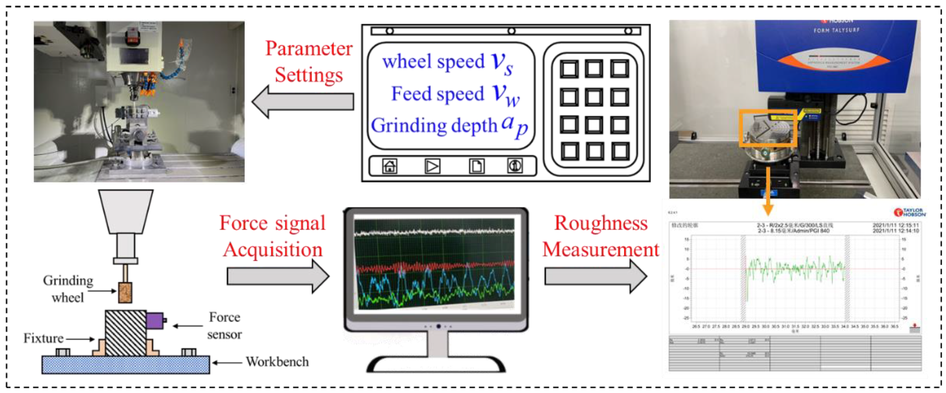
A CNC milling machine was used for grinding experiments. First, the test piece was bonded to the iron plate fixed on the milling machine to ensure the synchronous movement of the test piece and the worktable. Then, the triaxial force sensor fixed on the iron plate detected the force of the specimen; the specific experimental process is shown in Figure 1.
Figure 1.
Experimental flow.
2.2. Data Processing and Selection
The grinding force signal is closely related to the wear of the grinding wheel. Therefore, it is a feasible approach to extract the features of grinding wheel wear through the normal force data and obtain parameters for the subsequent BPNN prediction, extracting features in time, frequency, and time–frequency domains to retain as many features of the normal force signal as possible. Due to the large amount of experimental data, 20,000 data points in the smooth grinding state were selected for analysis in each group of experiments.
Due to machine tool vibration and ambient temperature, there was a lot of noise interference in the collected normal force signal, which affected subsequent feature analysis. Therefore, noise reduction and zero-drift compensation were performed on the normal force signal to reduce the impact of the environment and ensure a high signal-to-noise ratio of the signal. According to the experimental environment, the force signal was processed by low-pass filtering with a cutoff frequency of 500 Hz. Finally, the features of grinding wheel wear were determined in the time domain, frequency domain, and time–frequency domain, as shown in Table 2.
Table 2.
Relevant features of grinding wheel wear.
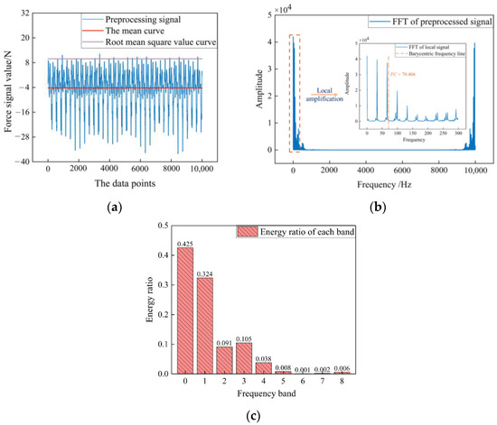
Figure 2 shows the processing of the normal force signal. In the time domain and frequency domain, the mean value AVG, the root mean square value RMS, and the barycenter frequency FC were often used to characterize grinding wheel wear. In the time–frequency domain, wavelet packet decomposition was used to analyze the non-stationary signals. From the frequency domain analysis, it was known that 0–62.5 Hz is the main frequency band of the normal force signal, and the four-layer wavelet packet decomposition was performed on this frequency band to observe the change of the energy ratio of the first eight frequency bands. By comparison, it was found that the energy of the fourth frequency band (16.5–19.5 Hz) and the total energy of the first eight frequency bands (0–31.25 Hz) were sensitive to grinding wheel wear. Therefore, the energy value ratios of the above two frequency bands were selected as the time–frequency domain features of grinding wheel wear.
Figure 2.
Processing of the normal force data: (a) time domain analysis of the normal force data; (b) frequency domain analysis of the normal force data; (c) time–frequency domain analysis of the normal force data.
According to the processed data, the parameters of the input layer are shown in Table 3. The processed data was divided into training samples and testing samples according to the principle of 3:1, which was convenient for the training and testing of the BP prediction model of ground surface roughness.
Table 3.
Input parameters of the prediction model.
3. Presented BP Neural Network Prediction Model
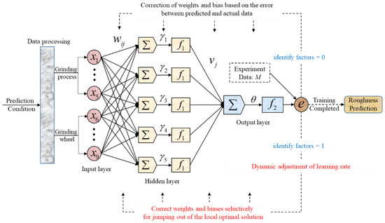
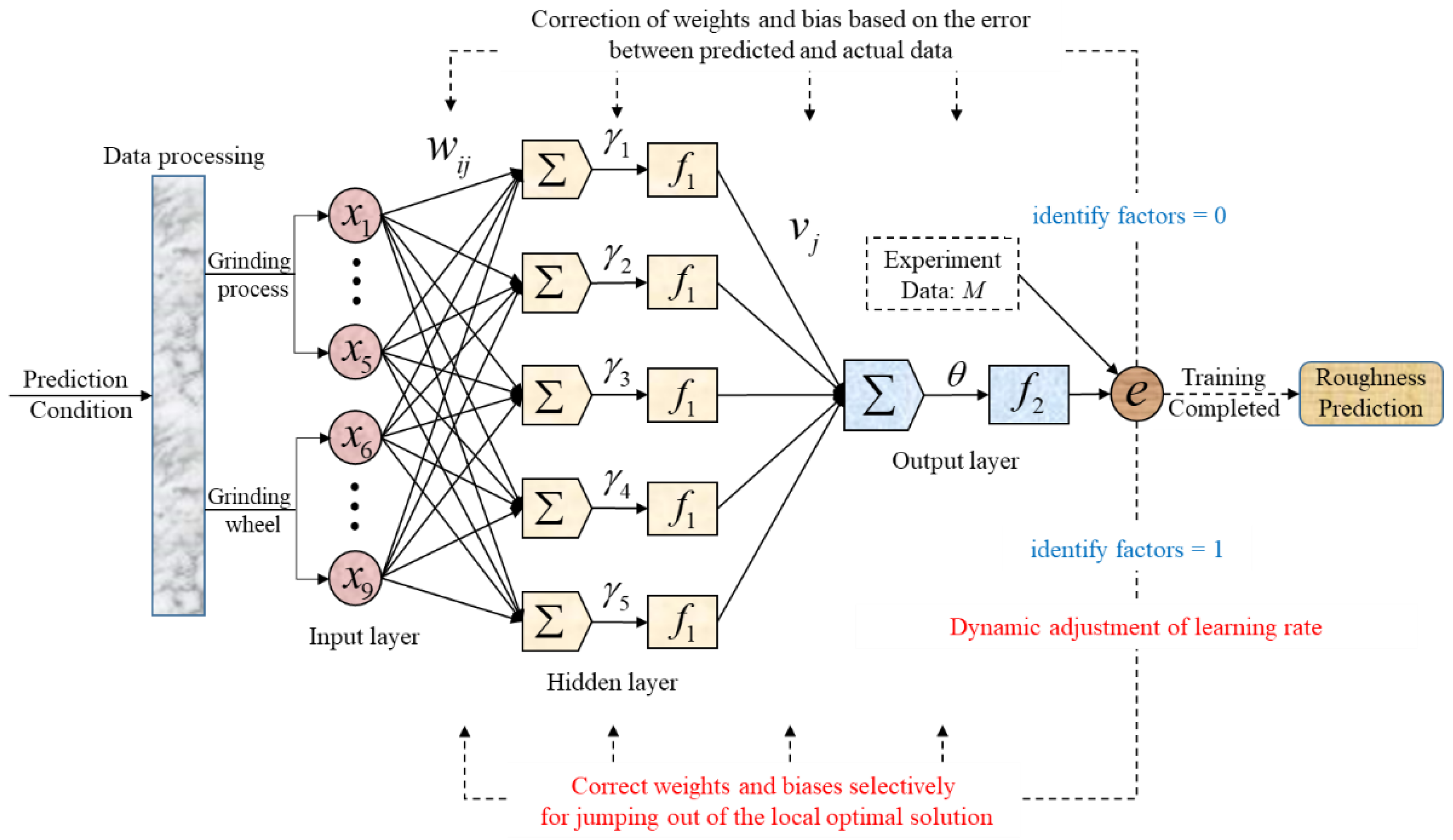
The core content of the BP algorithm is to update the parameters through gradient descent and error back propagation to find the optimal result for the entire path. When predicting ground surface roughness, the BP model can be trained by a certain number of training samples to fit the relationship between the ground surface roughness and grinding parameters under specific processing conditions. The presented BP prediction model of ground surface roughness with a single hidden layer constructed in this paper is shown in Figure 3.
Figure 3.
Presented BP neural network with single hidden layer.
According to the basic principle of BPNN, compared with multiple hidden layers, the BPNN with a single hidden layer is simpler and has the property of fitting nonlinear functions well. The number of nodes in the input layer depends on the dimension of the input samples; the parameters of the input layer are shown in Table 3. The number of nodes in the output layer is 1, and the output is the predicted value of the surface roughness Ra. The number of hidden layer nodes is determined through the principle of the golden section method:
where h is the number of hidden layer nodes, m is the number of input layer nodes, n is the number of output layer nodes, and a is an adjustment constant from 1 to 10. In this work, a is set as 5 − , and the number of hidden layer nodes h is 5.
In addition, the activation function of the hidden layer of the prediction model is the Sigmoid function, the activation function of the output layer is the identity function, and the error function is the global mean square error. The default learning rate μ is 0.024, the initial weights and biases are generated randomly, and the learned function is used to update the weights and biases of each layer.
3.1. The Standard BP Algorithm
The input layer vector of the neural network is x = (x1, x2, ⋯, x9), the hidden layer vector is y = (y1, y2, ⋯, y5), and w and γ represent the connection weights and biases between the input layer and the hidden layer. The output layer vector is z, whilst v and θ represent the connection weights and biases between the hidden layer and the output layer. The activation functions of the hidden layer and output layer are f1, f2.
The information forward propagation process of the neural network can be expressed as
After the BPNN completes the forward propagation of the information once, the back propagation of the error is carried out. First, the error function of the neural network is calculated:
where e is the error function and M is the expected output vector.
According to the negative gradient direction of the error function e, the connection weights and biases between the hidden layer and the output layer are updated:
where μ is the learning rate.
The connection weights and biases between the input layer and the hidden layer are then updated; the process is shown in Figure 3.
The above is an iterative process of the BPNN. The training and prediction of the model can be achieved by setting the number of iterations or the threshold of the error function e.
Finally, the developed predictive model can be represented by Equation (9):
3.2. The Local Optimal Solution
Based on the mathematical theory, the BPNN uses the local gradient feature of the error function to update the weights within finite iterative steps, and finally obtains the minimum training function value. However, the minimum training function value found is not necessarily the global optimal solution. From the perspective of the training function, there are multiple local optimal solutions instead of global optimal solutions, so the algorithm finally finds a local optimal solution with a high probability. From the perspective of the gradient descent method, the adjustment principle of the weights is based on local optima, and there is no algorithmic idea to avoid the local optima. When the initial weights and biases are determined, the local optimal solution is also determined, which is an important reason why many types of neural networks are difficult to optimize. The selection of initial weights and learning rate are two main factors that affect the generation of local optimal solutions. The initial weight is a sensitive parameter of the BP network, and different initial weights often cause the model to fall into different local optimal solutions. The learning rate affects the convergence characteristics of the neural network. When the learning rate is too large, the BP network may not converge, or converge rapidly in the early iteration, but may skip the local optimal solution and the global optimal solution in the later iteration, which will result in a decrease in the accuracy of the prediction model. When the learning rate is too small, the iteration of the BP network is slow, which reduces the efficiency of model and makes the model fall into the local optimal solution.
3.3. The Development of the Presented BP Algorithm
The traditional model does not judge the state of the network, it will iterate until the end of training. To solve the local optimal solution, a network state identification method is proposed in this paper. First, “identify factors” are designed to determine whether the BP network falls into the local optimal solution. Then, “memory factors” are designed to dynamically update and store the best weights during training. It is stipulated that after the error function value oscillates continuously three times during model training, “identify factors” is 1 and the BP network is considered to fall into the local optimal solution. In the rest of the cases, “identify factors” is 0.
where eN is the error value of the Nth training; eN−1 is the error value of the (N − 1)th training; and t − 1, t, and t + 1 are three consecutive positive integers. The “identify factors” are used to solve the convergence and local optimal problems later.
A fixed learning rate μ in traditional model cannot guarantee fast convergence and accurate prediction of the BPNN at the same time. Therefore, according to the different characteristics of the BP network in the early iteration and later iteration, the learning rate μ is adjusted dynamically. We judge the iterative state of the BPNN via “identify factors”: early iteration and later iteration. In the early iteration, the learning rate μ is kept at the default value, which improves the convergence speed and results in quickly approaching the optimal solution area. In the later iteration, “identify factors” = 1 and the learning rate μ decays through the Equation (11), which will improve the solution accuracy and avoid model oscillation:
To ensure that the learning rate μ decays moderately, h is set as the number of adjustments; the values are 0, 1, 2.
After falling into the local optimal solution, the traditional model does not process and continues to iterate until the end of training. In this paper, when h = 2, the learning rate μ is reset to the default value, h is reset to 0, and random oscillation is loaded on the weights of each layer in “memory factors”, so that the model avoids the local optimal solution:
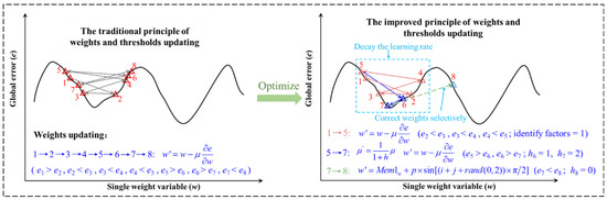
Mem1 and Mem2 are the weight matrices of the hidden layer and the output layer in “memory factors”. p is a random number in (0, 2) which represents the range of the random change of the weights. The sin function represents the direction in which the weights randomly change. i, j, and rand (0, 2) represent random changes between different weights. Then BP network is trained with wij and vj as the weights of each layer. After the training, the best weights in “memory factors” are taken as the final solution. The comparison of the traditional and proposed updating principle of the weights and thresholds is shown in Figure 4.
Figure 4.
Comparison of the traditional and improved updating principle of the weights and thresholds.
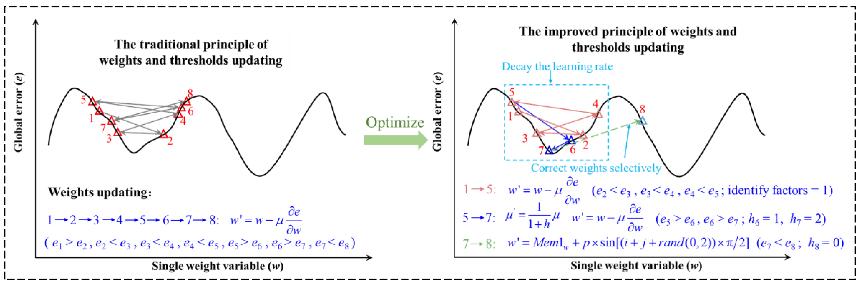
In the training process of the presented BP, the adjustment of the learning rate and update of the weights are influenced mutually. The change of the learning rate affects the result of the weight update, and the update of the weights affects the iterative state of the network, which in turn affects the value of the “identify factors” and finally affects the change of the learning rate. The specific process of the prediction model of ground surface roughness is shown in Figure 5.
Figure 5.
The process of predicting ground surface roughness.
3.4. The Performance Evaluation of the Presented BP
The prediction performance of the presented BP network for ground surface roughness is evaluated from two aspects: firstly, analyzing the influence of grinding wheel wear parameters on the prediction model of ground surface roughness; secondly, comparing the prediction performance of the BP network before and after optimization.
The traditional BP network is used to predict the ground surface roughness to analyze the influence of grinding wheel wear, and the global relative error is used as the measurement index of the prediction accuracy:
where δ is the global relative error, N is the number of the testing samples, and μi and xi are the measured and predicted values of the surface roughness of the ith sample in the testing samples.
Comparing the prediction performance of the BP network before and after optimization, Equation (14) is used as the measurement index of the prediction accuracy, and the standard deviation is used as the measurement index of the stability of the prediction model:
where s is the sample standard deviation and δi is the relative error of the predicted value of the ith sample in the testing samples.
4. Results and Discussion
4.1. Influence of Grinding Wheel Wear Features
The traditional BP network was used to predict the ground surface roughness to verify the influence of grinding wheel wear parameters. The basic process parameters in Table 3 were selected as the input parameters of the neural network—Traditional BP1 (Tra BP1), and all the parameters in Table 3 are the input parameters of the neural network—Traditional BP2 (Tra BP2). The number of input layer nodes of Traditional BP1 and Traditional BP2 are 5 and 9, respectively, whilst the other parameters are set to be the same. The number of nodes in the hidden layer and output layer are 5 and 1, respectively; the default learning rate is 0.024; and the three types of iteration steps K are set to 2000, 10,000, and 15,000.
Both models were trained with training samples and then tested 20 times with testing samples for three types of iterative steps. The relative error has been used to characterize the prediction accuracy; the results are shown in Table 4, whilst the experimental results and predicted results appear in Appendix A at the end of the paper.
Table 4.
Influence of grinding wheel wear features on prediction results.
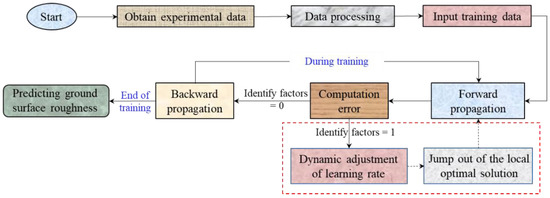
After the grinding wheel wear features were introduced, the best prediction accuracy of surface roughness Ra improved from 0.062, 0.062, 0.061 to 0.045, 0.035, 0.031, respectively. The average prediction accuracy also improved, from 0.071, 0.065, 0.066 to 0.050, 0.053, 0.054, respectively. The BP prediction model is essentially an optimal nonlinear function that maps input parameters to output parameters. The results show that the wear characteristics of the grinding wheel enhance the correlation between the input parameters and the ground surface roughness and promote the development of the BP model during iterative training: the update of the weights and biases of each layer. According to the physical model, the increase in the dimension of the input parameters improves the mapping ability of the model (the best prediction accuracy of the BP network).
The specific data of the relative prediction error of Traditional BP1 and Traditional BP2 are shown in Figure 6. Compared with K = 10,000 and K = 15,000, the prediction accuracy of Traditional BP1 is fluctuates more when K = 2000. Because the number of iterations is too small, the training level of the Traditional BP1 is low, and a good mapping relationship between the input parameters and the surface roughness Ra cannot be established. However, the prediction accuracy of Traditional BP2 tends to be stable and is significantly higher than that of Traditional BP1. Because the grinding wheel wear features enhance the mapping relationship between input and output, high prediction accuracy is achieved with fewer iteration steps.
Figure 6.
Influence of grinding wheel wear features on the prediction accuracy of the model.
As the number of iteration steps increases, the prediction accuracy of Traditional BP1 gradually stabilizes around 0.065, which indicates that the model has reached a saturated training level. However, the fluctuation of the prediction accuracy of Traditional BP2 becomes larger, which is caused by overfitting. Because after the model training is saturated, continuing to iterate will reduce the generalization and lead to overfitting. At the same time, the increase of the input parameter dimension and the randomness of the initial weight will make the model more likely to fall into the local optimal solution. This is a typical defect of the traditional BPNN, which is the problem that the next section focuses on solving.
In summary, the selected grinding wheel wear features enhance the correlation between the input parameters and the ground surface roughness and improves the mapping ability and prediction performance of the model. However, it makes the model fall into the local optimal solution more easily.
4.2. Comparison of Prediction Models before and after Optimization
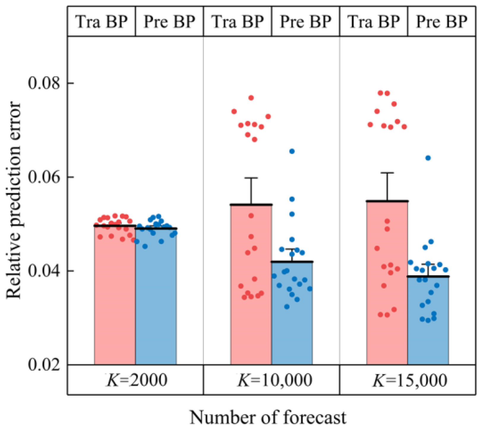
Section 4.1 proves the effect of grinding wheel wear, but the local optimal solution and over-convergence of the BP model become more serious due to the increase of the input dimension. Based on it, the iterative termination conditions of the prediction model, the weight update rules, and learning rate should be improved. To compare the prediction performance of the BP network before and after optimization, all the parameters in Table 3 are selected as the input parameters of the traditional BP network—Traditional BP (Tra BP) and the presented BP network—Presented BP (Pre BP). The number of input layer, hidden layer, and output layer nodes of both are 9, 5, and 1, respectively; the default learning rate is 0.024; the three types of iteration steps K are set to 2000, 10,000, and 15,000; and the initial weights are the same and generated randomly. The training and prediction process of the two models is the same as in Section 4.1; the results are shown in Figure 7, whilst the experimental results and predicted results appear in Appendix B at the end of the paper.
Figure 7.
Comparison of prediction accuracy of the traditional model and the presented model.
4.2.1. Influence of “Identify Factors”
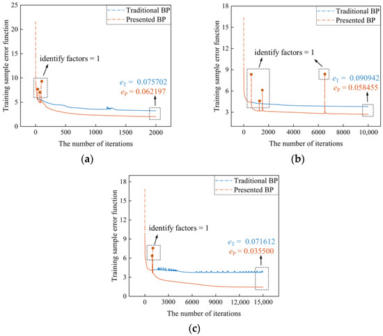
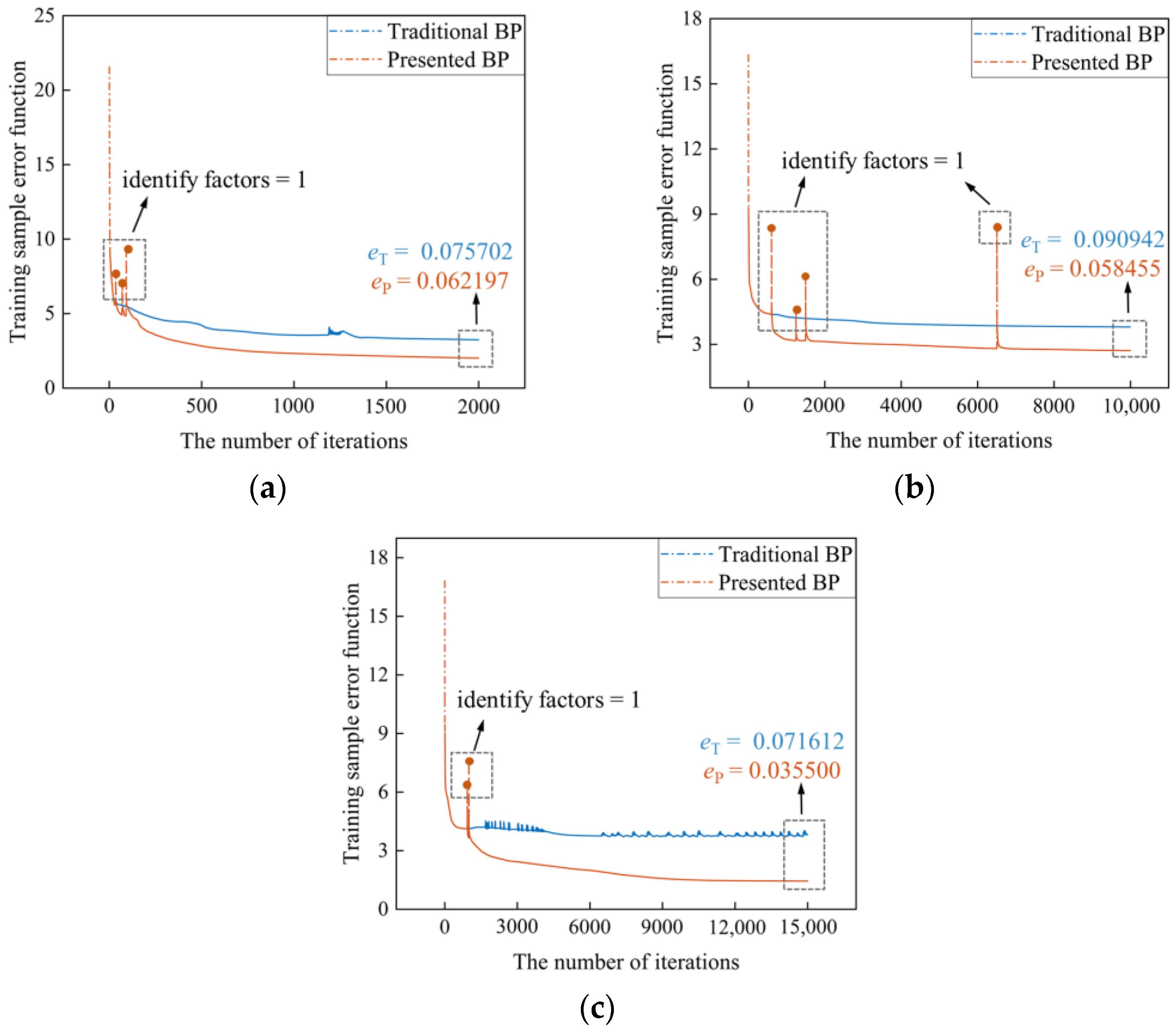
The error functions in the training of the Traditional BP and Presented BP were analyzed, as shown in Figure 8. In the early iteration, the error functions of both decrease rapidly. In the later iteration, the error function curve of Traditional BP decreases very slowly, while that of Presented BP changes suddenly and then decreases rapidly. Under the same number of iteration steps, the error function value eP of Presented BP is smaller than the error function value eT of Traditional BP, and the final training accuracy of Presented BP is higher. Because the two models deal with the local optimal solution problem differently during training. After falling into the local optimal solution, Traditional BP does not process and continues to iterate until the end of training. Presented BP judges the network state by “identify factors”. When “identify factors” = 1, the network falls into the local optimal solution, and the model begins to dynamically adjust the learning rate and selectively update the weights of each layer, avoiding the local optimal solution and continuing to search for the global optimal solution. Hence, the “identify factors” in this paper can effectively determine whether the BP network falls into the local optimal solution, which is a good remedy for the defects of the BP algorithm; Presented BP can completely solve the global optimal solution in the training process.
Figure 8.
The error function of the traditional model and the presented model during training: (a) the number of iteration steps K of the models is 2000; (b) the number of iteration steps K of the models is 10,000; (c) the number of iteration steps K of the models is 15,000.
4.2.2. Influence of Dynamic Learning Rate
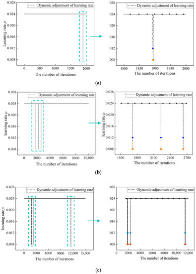
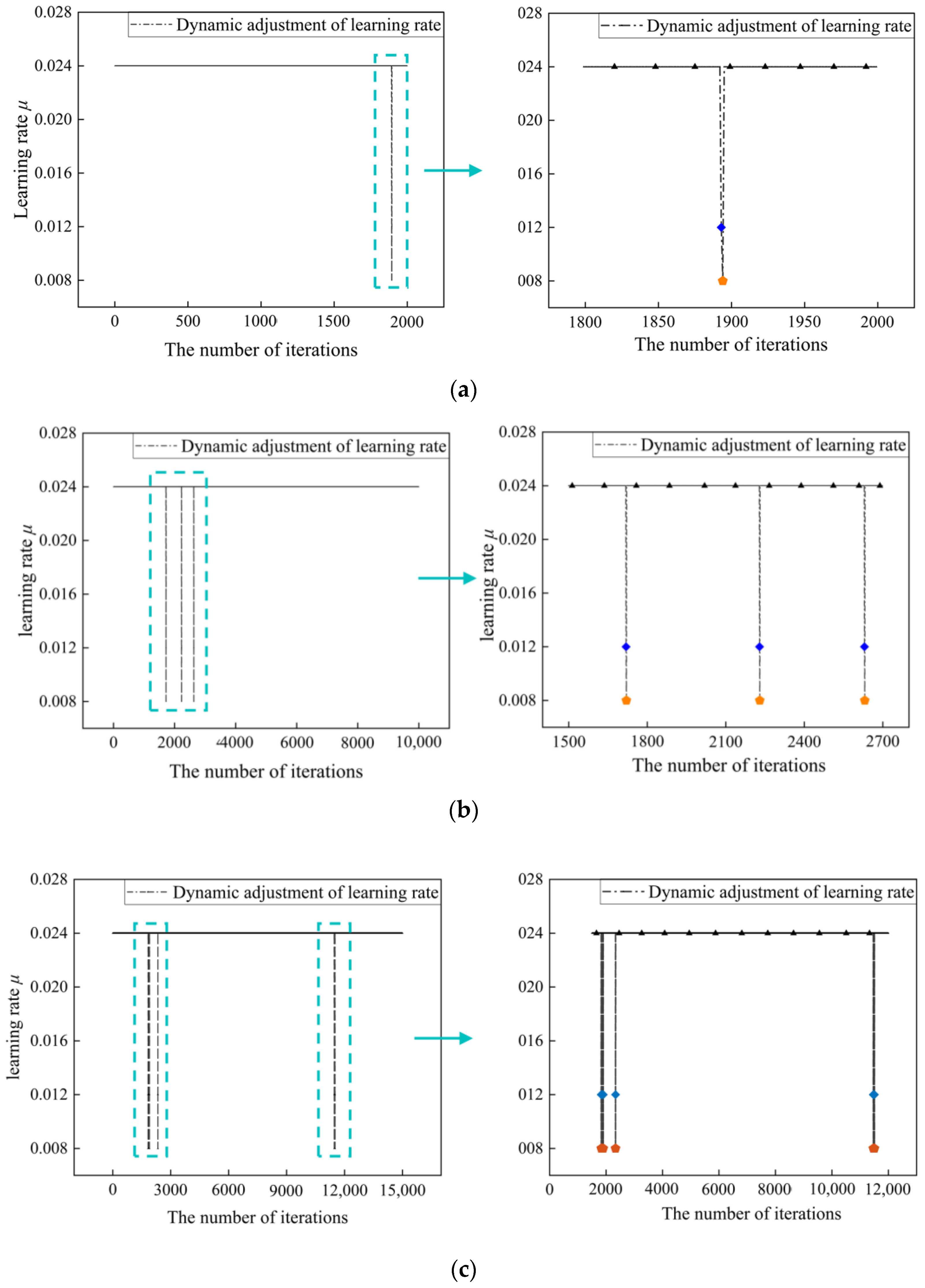
Figure 9 shows the change in learning rate in the training of the Presented BP. During training, the learning rate μ of Presented BP changes dynamically at a specific iteration step, decaying from 0.024 to 0.012 and eventually to 0.008 at the end. According to the principle of the optimized algorithm, in the early iteration, the learning rate μ is kept at the default value, so that the model converges quickly to a local optimal solution. In the later iteration, after “identify factors” judges that the network is falling into the local optimal solution, the learning rate μ is dynamically attenuated according to Equation (11), which slows down the magnitude of weight update and improves the accuracy of the target weights. After the network avoids the local optimal solution, the learning rate μ is reset to the default value to adapt to the next early iteration. The dynamic learning rate not only ensures the training efficiency of the prediction model, but also improves the accuracy of the target weights.
Figure 9.
Dynamic change of the learning rate in the presented model during training: (a) the number of iteration steps K of the models is 2000; (b) the number of iteration steps K of the models is 10,000; (c) the number of iteration steps K of the models is 15,000.
4.2.3. Comparison of Prediction Accuracy
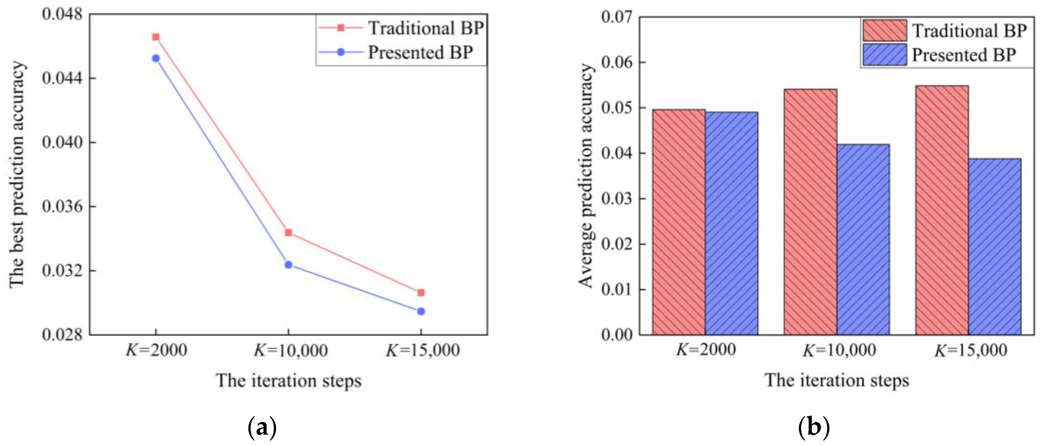
Under three types of iteration steps, the prediction accuracy of Traditional BP and Presented BP are compared, as shown in Figure 10. Under the iteration steps of K = 2000, K = 10,000, and K = 15,000, the best prediction accuracy of Traditional BP is 0.0466, 0.0344, and 0.0306, while that of Presented BP is 0.0452, 0.0324, and 0.0295, respectively. The difference between the best prediction accuracy of the two models is small because under the same number of iteration steps, the dimension and feature quantity of the input parameters are the main factors, which affect the best prediction accuracy of the BP model. However, the accuracy of Presented BP is slightly higher because in the early iteration of network training, the two models have not fallen into the local optimal value, and are iterated and updated in the same way. When both fall into the same local optimal solution, Traditional BP is limited by its own algorithm and does not process until the end of training. However, Presented BP judges the network state through “identify factors”, and dynamically adjusts the learning rate μ (which reduces the weight update range and improves the solution accuracy of the target weights) and selectively updates the weights (which makes the model avoid the local optimal solution, in order to search for the global optimal solution until the end of training). Presented BP can continuously search for the global optimal value, so its best prediction accuracy is improved.
Figure 10.
Comparison of the prediction accuracy of the traditional model and the presented model: (a) the best prediction accuracy of the models; (b) the average prediction accuracy of the models.
With the increase of the number of iteration steps, the average prediction accuracy of Traditional BP decreases (0.050, 0.054, and 0.055) while that of Presented BP increases (0.049, 0.042, and 0.039). During the training process, after falling into the local optimal solution, Traditional BP continues to iterate and results in overfitting, which reduces the generalization and prediction accuracy of the model. However, there is no over-convergence phenomenon in Presented BP. As the number of iteration steps increases, Presented BP will continue to avoid the local optimal solution and search for the global optimal solution, so the average prediction accuracy will be improved.
4.2.4. Comparison of Predictive Stability
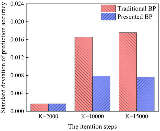
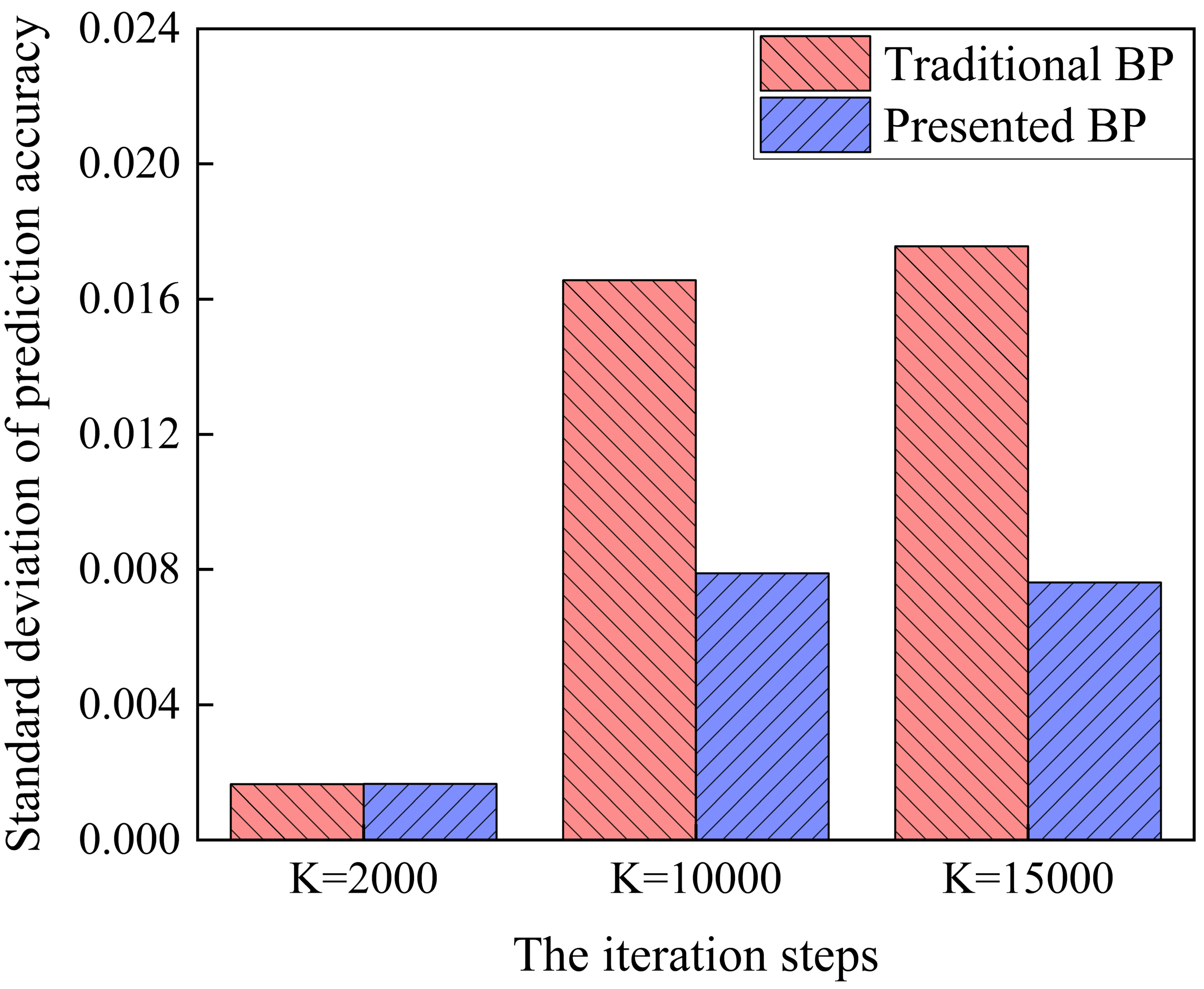
Under three types of iteration steps, the prediction stability of Traditional BP and Presented BP is compared, as shown in Figure 11. Under the iteration steps of K = 2000, K = 10,000, and K = 15,000, the prediction standard deviations of Traditional BP and Presented BP are 0.0017, 0.0166, 0.0175 and 0.0017, 0.0079, 0.0076, respectively. As the number of iteration steps increases, the prediction stability of Presented BP is significantly better. Because the algorithm structure of Presented BP is more reasonable, the dynamic learning rate and the improved weight update rules avoid the model falling into the local optimal solution and keep the prediction stable. When the input parameters are unchanged, the prediction performance of Traditional BP mainly depends on the fixed learning rate and initial weight, so the stability is extremely poor. As the number of iteration steps increases, the over-convergence phenomenon of Traditional BP is more serious, and the prediction fluctuation is bigger. In summary, as the number of iteration steps increases, Presented BP continuously avoids the local optimal solution and the dependence of the model on the initial weights decreases, so the stability of the prediction accuracy improves.
Figure 11.
Comparison of prediction standard deviations of the traditional model and the presented model.
5. Conclusions
Based on the physical model of ground surface roughness, this paper proposes an adaptive BP network prediction model considering grinding wheel wear. However, the increase of input parameter dimension makes the problem of local optimal solution of BP network more serious. In this situation, improving the iterative termination conditions of the prediction model, dynamically decaying the learning rate, and adjusting the weight update rules help to solve the problem of local optimal solutions. Comparing the prediction performance of the presented BP network and the traditional BP network, the results show the following:
- (1)
- The features of the force signal selected in this paper contain enough grinding wheel state information, which enhances the correlation between the input parameters and the ground surface roughness Ra and improves prediction performance of the model.
- (2)
- The “identify factors” effectively judge whether the BP network falls into the local optimal solution and reduces the influence of human factors. The “memory factors” can update and store the best weights in real time during network training.
- (3)
- The improvement of the iterative termination conditions of the prediction model and the adjustment of the weight update rules are effective measures for solving the local optimal solution problem, reducing the influence of human factors, and maximizing the prediction performance of the model itself. Dynamic adjustment of learning rate improves the search accuracy of the target weights with the premise of ensuring rapid convergence.
In summary, the presented BP prediction model of ground surface roughness considering grinding wheel wear not only greatly improves the prediction accuracy, but also significantly enhances the prediction stability.
Author Contributions
Funding acquisition, P.Z.; supervision, Y.Y. and P.Z.; validation, X.L., Y.P. and Y.W.; writing—original draft preparation, X.L.; writing—review and editing, X.L., Y.P., Y.Y., Y.W. and P.Z. All authors have read and agreed to the published version of the manuscript.
Funding
This research was funded by The National Natural Science Foundation of China (No. 51875078, No. 51991372, No. 51975094), and the Science Fund for Creative Research Groups of NSFC of China (No. 51621064).
Institutional Review Board Statement
Not applicable.
Informed Consent Statement
Not applicable.
Data Availability Statement
All data generated or analyzed during this study are included in the present article.
Acknowledgments
The authors appreciate the financial support from the National Natural Science Foundation of China and the Science Fund for Creative Research Groups of NSFC of China.
Conflicts of Interest
The authors declare no conflict of interest.
Appendix A
Appendix A.1
| Data Number | Wheel Speed vs (rpm) | Workpiece Speed vw (mm/min) | Depth of Cut ap (μm) | Normal Force Fn (N) | Tangential Force Ft (N) | Experimental Value Ra (μm) |
| 1 | 500 | 100 | 50 | 11.9 | 3 | 6.1736 |
| 2 | 500 | 100 | 50 | 51 | 7.4 | 11.1541 |
| 3 | 500 | 100 | 50 | 103 | 5 | 21.9520 |
| 4 | 500 | 200 | 100 | 34.8 | 10.3 | 10.2449 |
| 5 | 500 | 200 | 100 | 100 | 9.2 | 18.3258 |
| 6 | 500 | 200 | 100 | 151 | 17 | 26.6484 |
| 7 | 500 | 500 | 150 | 72.7 | 29.6 | 15.2052 |
| 8 | 500 | 500 | 150 | 167 | 42.6 | 25.1561 |
| 9 | 500 | 500 | 150 | 321 | 50 | 48.0556 |
| 10 | 2000 | 100 | 100 | 4.3 | 1.5 | 6.1047 |
| 11 | 2000 | 100 | 100 | 78 | 9 | 17.0280 |
| 12 | 2000 | 100 | 100 | 103 | 13 | 20.9814 |
| 13 | 2000 | 200 | 150 | 18 | 5.1 | 8.1575 |
| 14 | 2000 | 200 | 150 | 72 | 14.4 | 13.9500 |
| 15 | 2000 | 200 | 150 | 136 | 27.6 | 26.1880 |
| 16 | 2000 | 500 | 50 | 14.3 | 3.7 | 7.7320 |
| 17 | 2000 | 500 | 50 | 75 | 7.2 | 14.0218 |
| 18 | 2000 | 500 | 50 | 105 | 17.5 | 17.9756 |
| 19 | 5000 | 100 | 150 | 24 | 4.8 | 10.8010 |
| 20 | 5000 | 100 | 150 | 42.3 | 13.3 | 11.5534 |
| 21 | 5000 | 200 | 50 | 4.13 | 1 | 7.1582 |
| 22 | 5000 | 200 | 50 | 11.7 | 1.8 | 8.2657 |
| 23 | 5000 | 200 | 50 | 4.3 | 1 | 9.1648 |
| 24 | 5000 | 500 | 100 | 9.5 | 3.3 | 11.6318 |
| 25 | 5000 | 500 | 100 | 42 | 8.2 | 11.6829 |
| 26 | 5000 | 500 | 100 | 93 | 26 | 19.8032 |
Appendix A.2
| Data Number | Experimental Value Ra (μm) | Traditional BP1—Predictive Value Ra (μm) | Traditional BP2—Predictive Value Ra (μm) | ||||
| K = 2000 | K = 10,000 | K = 15,000 | K = 2000 | K = 10,000 | K = 15,000 | ||
| 1 | 6.1736 | 5.9377 | 6.0387 | 6.2356 | 6.1662 | 6.1155 | 6.1012 |
| 2 | 11.1541 | 12.0337 | 11.6825 | 11.5120 | 10.5000 | 11.1706 | 11.2820 |
| 3 | 21.9520 | 21.5702 | 21.2504 | 21.2368 | 20.5791 | 22.4294 | 22.5386 |
| 4 | 10.2449 | 10.0019 | 10.3689 | 10.4252 | 9.8667 | 10.3491 | 10.3809 |
| 5 | 18.3258 | 18.8424 | 19.2144 | 19.2610 | 18.7863 | 18.9356 | 19.0346 |
| 6 | 26.6484 | 28.3290 | 28.2966 | 28.7689 | 25.2541 | 27.1364 | 27.2721 |
| 7 | 15.2052 | 15.0605 | 15.2562 | 15.1439 | 15.4312 | 16.1145 | 16.1340 |
| 8 | 25.1561 | 25.2395 | 24.9701 | 24.9139 | 23.5573 | 24.5187 | 24.5491 |
| 9 | 48.0556 | 46.0416 | 47.0087 | 45.4198 | 45.3688 | 46.1008 | 46.2746 |
| 10 | 6.1047 | 6.4816 | 6.6989 | 6.6483 | 6.2067 | 5.8297 | 5.7838 |
| 11 | 17.0280 | 17.2812 | 16.7244 | 16.4367 | 15.6231 | 16.6271 | 16.5679 |
| 12 | 20.9814 | 24.2625 | 21.6212 | 21.7584 | 22.9222 | 22.8483 | 23.1165 |
| 13 | 8.1575 | 9.2555 | 8.8188 | 8.8718 | 8.2594 | 8.7358 | 8.7104 |
| 14 | 13.9500 | 14.5951 | 14.4810 | 14.2326 | 13.4412 | 13.9532 | 13.9405 |
| 15 | 26.1880 | 24.8701 | 23.6104 | 24.0026 | 22.1440 | 22.6590 | 22.6393 |
| 16 | 7.7320 | 7.5589 | 7.3077 | 7.1534 | 6.4606 | 6.8010 | 6.7185 |
| 17 | 14.0218 | 14.4235 | 14.1043 | 14.0486 | 13.1745 | 13.8179 | 13.8261 |
| 18 | 17.9756 | 19.3721 | 19.6324 | 19.6932 | 16.7902 | 17.5231 | 17.5951 |
| 19 | 10.8010 | 11.7955 | 12.0829 | 12.0662 | 11.1319 | 11.3751 | 11.2238 |
| 20 | 11.5534 | 14.1061 | 13.4673 | 13.4241 | 12.1707 | 12.7432 | 12.7371 |
| 21 | 7.1582 | 8.1107 | 7.2854 | 7.1587 | 6.7721 | 6.8446 | 6.6590 |
| 22 | 8.2657 | 9.1981 | 8.7790 | 8.5764 | 9.1519 | 8.8483 | 8.7494 |
| 23 | 9.1648 | 8.1302 | 7.3138 | 7.1842 | 7.8731 | 9.9086 | 10.0518 |
| 24 | 11.6318 | 11.7538 | 11.9479 | 11.8384 | 10.6782 | 12.6480 | 12.3767 |
| 25 | 11.6829 | 14.1239 | 13.1856 | 12.8342 | 11.3742 | 11.3799 | 11.3417 |
| 26 | 19.8032 | 19.3947 | 19.2437 | 19.2250 | 18.7686 | 19.7676 | 19.6758 |
Appendix B
| Data Number | Experimental Value Ra (μm) | Traditional BP—Predictive Value Ra (μm) | Presented BP—Predictive Value Ra (μm) | ||||
| K = 2000 | K = 10,000 | K = 15,000 | K = 2000 | K = 10,000 | K = 15,000 | ||
| 1 | 6.1736 | 6.4858 | 6.0926 | 6.1053 | 6.4803 | 6.3844 | 6.3914 |
| 2 | 11.1541 | 11.0681 | 11.1851 | 11.3842 | 11.0661 | 11.0914 | 11.1930 |
| 3 | 21.9520 | 21.6907 | 22.2608 | 22.2202 | 21.8527 | 22.7907 | 22.5332 |
| 4 | 10.2449 | 10.3773 | 10.3049 | 10.3420 | 10.3619 | 10.3389 | 10.2789 |
| 5 | 18.3258 | 18.8043 | 19.4418 | 19.3012 | 18.8031 | 18.7728 | 18.6973 |
| 6 | 26.6484 | 26.4874 | 26.9640 | 27.3843 | 26.4996 | 26.9174 | 26.8206 |
| 7 | 15.2052 | 16.2578 | 16.1387 | 16.4480 | 16.2493 | 15.9223 | 15.9661 |
| 8 | 25.1561 | 24.8344 | 24.6758 | 24.8958 | 24.8125 | 24.7823 | 24.8555 |
| 9 | 48.0556 | 47.7151 | 46.1312 | 47.2702 | 47.9425 | 46.3802 | 45.8345 |
| 10 | 6.1047 | 6.5375 | 5.7150 | 5.7788 | 6.5362 | 6.2685 | 6.2314 |
| 11 | 17.0280 | 16.4552 | 16.6609 | 16.4891 | 16.4355 | 16.4205 | 16.4199 |
| 12 | 20.9814 | 22.9105 | 21.7201 | 21.6857 | 22.9364 | 21.2162 | 21.2612 |
| 13 | 8.1575 | 8.7020 | 8.7292 | 8.7220 | 8.6979 | 8.5404 | 8.6626 |
| 14 | 13.9500 | 14.1399 | 14.0282 | 13.9418 | 14.1267 | 14.0676 | 14.1740 |
| 15 | 26.1880 | 23.3289 | 22.7952 | 23.4145 | 23.3002 | 23.0938 | 23.7798 |
| 16 | 7.7320 | 6.7857 | 6.7942 | 6.8517 | 6.7897 | 6.6948 | 6.6982 |
| 17 | 14.0218 | 13.8670 | 13.8426 | 13.9006 | 13.8532 | 13.9206 | 13.9464 |
| 18 | 17.9756 | 17.6694 | 17.5528 | 17.6178 | 17.6093 | 17.3578 | 17.4885 |
| 19 | 10.8010 | 11.6912 | 11.4173 | 11.3406 | 11.6866 | 11.1868 | 11.0692 |
| 20 | 11.5534 | 12.7916 | 12.6634 | 12.7060 | 12.7486 | 12.7000 | 12.6143 |
| 21 | 7.1582 | 7.1516 | 6.8157 | 6.5673 | 7.1731 | 6.9274 | 6.9051 |
| 22 | 8.2657 | 9.6312 | 8.9185 | 8.8806 | 9.6243 | 8.6722 | 8.4149 |
| 23 | 9.1648 | 8.3259 | 10.4199 | 10.7947 | 8.4040 | 9.0801 | 9.2246 |
| 24 | 11.6318 | 11.2833 | 12.8674 | 12.5209 | 11.2640 | 11.2953 | 11.4915 |
| 25 | 11.6829 | 11.9769 | 11.4133 | 11.3775 | 11.9692 | 11.5338 | 11.5788 |
| 26 | 19.8032 | 19.7932 | 19.6678 | 20.0712 | 19.8338 | 19.9598 | 19.9507 |
References
- Lin, X.K.; Li, H.L.; Yuan, B. Research on PSO-SVR based Intelligent Prediction of Surface Roughness for CNC Surface Grinding Process. J. Syst. Simul. 2009, 21, 7805–7808. [Google Scholar]
- Pan, Y.H.; Wang, Y.H.; Zhou, P. Activation functions selection for BP neural network model of ground surface roughness. J. Intell. Manuf. 2020, 31, 1825–1836. [Google Scholar] [CrossRef]
- Pan, Y.H.; Zhou, P.; Yan, Y. New insights into the methods for predicting ground surface roughness in the age of digitalisation. Precis. Eng. 2021, 67, 393–418. [Google Scholar] [CrossRef]
- Fountas, N.; Papantoniou, L.; Kechagias, J. Modeling and optimization of flexural properties of FDM-processed PET-G specimens using RSM and GWO algorithm. Eng. Fail. Anal. 2022, 138, 106340. [Google Scholar] [CrossRef]
- Fountas, N.; Papantoniou, L.; Kechagias, J. An experimental investigation of surface roughness in 3D-printed PLA items using design of experiments. J. Eng. Tribol. 2021, 135065012110593. [Google Scholar] [CrossRef]
- Asiltürk, İ.; Tinkir, M.; El Monuayri, H. An intelligent system approach for surface roughness and vibrations prediction in cylindrical grinding. Int. J. Comput. Integr. Manuf. 2012, 25, 750–759. [Google Scholar] [CrossRef]
- Yin, S.H.; Nguyen, D.; Chen, F.J. Application of compressed air in the online monitoring of surface roughness and grinding wheel wear when grinding Ti-6Al-4V titanium alloy. Int. J. Adv. Manuf. Technol. 2018, 101, 1315–1331. [Google Scholar] [CrossRef]
- Sudheer, K.; Varma, I.; Rajesh, S. Prediction of surface roughness and MRR in grinding process on Inconel 800 alloy using neural networks and ANFIS. Mater. Today Proc. 2018, 5, 5445–5451. [Google Scholar] [CrossRef]
- Liang, Z.W.; Liao, S.P.; Wen, Y.H. Working parameter optimization of strengthen waterjet grinding with the orthogonal-experiment-design-based ANFIS. J. Intell. Manuf. 2019, 30, 833–854. [Google Scholar] [CrossRef]
- Li, G.; Wang, L.; Ding, N. On-line prediction of surface roughness in cylindrical longitudinal grinding based on evolutionary neural networks. China Mech. Eng. 2005, 16, 223–226. [Google Scholar]
- Vaxevanidis, N.; Kechagias, J.; Fountas, N. Evaluation of Machinability in Turning of Engineering Alloys by Applying Artificial Neural Networks. Open Constr. Build. Technol. J. 2014, 8, 389–399. [Google Scholar] [CrossRef] [Green Version]
- Jiao, Y.; Ler, S.; Pei, Z.J. Fuzzy adaptive networks in machining process modeling: Surface roughness prediction for turning operations. Int. J. Mach. Tools Manuf. 2004, 44, 1643–1651. [Google Scholar] [CrossRef]
- Kechagias, J.; Fountas, Y.H.; Fountas, N. Surface characteristics investigation of 3D-printed PET-G plates during CO2 laser cutting. Mater. Manuf. Process. 2021, 1–11. [Google Scholar] [CrossRef]
- Baseri, H. Workpiece surface roughness prediction in grinding process for different disc dressing conditions. In Proceedings of the 2010 International Conference on Mechanical and Electrical Technology, Singapore, 10–12 September 2010; pp. 209–212. [Google Scholar]
- Shrivastava, Y.; Singh, B. Stable cutting zone prediction in CNC turning using adaptive signal processing technique merged with artificial neural network and multi-objective genetic algorithm. Eur. J. Mech. 2018, 70, 238–248. [Google Scholar] [CrossRef]
- Jiang, J.L.; Ge, P.Q.; Bi, W.B. 2D/3D ground surface topography modeling considering dressing and wear effects in grinding process. Int. J. Mach. Tools Manuf. 2013, 74, 29–40. [Google Scholar] [CrossRef]
- Zhou, J.H.; Pang, C.K.; Lewis, F.L. Intelligent Diagnosis and Prognosis of Tool Wear Using Dominant Feature Identification. IEEE Trans. Ind. Inform. 2009, 5, 454–464. [Google Scholar] [CrossRef]
- Elbestawi, M.A.; Marks, J.; Papazafiriou, T. Process Monitoring in Milling by Pattern-Recognition. Mech. Syst. Signal Process. 1989, 3, 305–315. [Google Scholar] [CrossRef]
- Yang, Z.X.; Yu, P.P.; Gu, J.N. Study on Prediction Model of Grinding Surface Roughness Based on PSO-BP Neural Network. Tool Eng. 2017, 51, 36–40. [Google Scholar]
- Li, S.; Liu, L.J.; Zhai, M. Prediction for short-term traffic flow based on modified PSO optimized BP neural network. Syst. Eng. Theory Pract. 2012, 32, 2045–2049. [Google Scholar]
- Li, Q.; Lin, Y.Q.; Yang, Y.P. Fault diagnosis method of wind turbine gearbox based on BP neural network trained by particle swarm optimization algorithm. Acta Energ. Sol. Sin. 2012, 33, 120–125. [Google Scholar]
- Pan, H.; Hou, Q.L. A BP neural networks learning algorithm research based on particle swarm optimizer. Comput. Eng. Appl. 2006, 16, 41–43. [Google Scholar]
- Wang, R.X.; Chen, B.; Qiu, S.H. Hazardous source estimation using an artificial neural network, particle swarm optimization and a simulated annealing algorithm. Atmosphere 2018, 9, 119. [Google Scholar] [CrossRef] [Green Version]
- Gao, H.B.; Gao, L.; Zhou, C. Particle swarm optimization based algorithm for neural network learning. Acta Electonica Sin. 2004, 32, 1572. [Google Scholar]
- Chen, M.R.; Chen, B.P.; Zeng, G.Q. An adaptive fractional-order BP neural network based on extremal optimization for handwritten digits recognition. Neurocomputing 2020, 391, 260–272. [Google Scholar] [CrossRef]
- Chu, L.N.; Chen, C.L. Design and Application of BP Neural Network Optimization Method Based on SIWSPSO Algorithm. Secur. Commun. Netw. 2022, 2022, 2960992. [Google Scholar] [CrossRef]
- Zhang, Y.H.; Hu, D.J.; Zhang, K. Prediction of the Surface Roughness in Curve Grinding Based on Evolutionary Neural Networks. J. Shanghai Jiaotong Univ. 2005, 39, 373–376. [Google Scholar]
- Liu, C.Y.; Ling, J.C.; Kou, L.Y. Performance comparison between GA-BP neural network and BP neural network. Chin. J. Health Stat. 2013, 30, 173–176. [Google Scholar]
- Wang, D.M.; Wang, L.; Zhang, G.M. Short-term wind speed forecast model for wind farms based on genetic BP neural network. J. Zhejiang Univ. 2012, 46, 837–841. [Google Scholar]
- Li, S.; Liu, L.J.; Xie, Y.L. Chaotic prediction for short-term traffic flow of optimized BP neural network based on genetic algorithm. Control Decis. 2011, 26, 1581–1585. [Google Scholar]
- Ding, S.F.; Su, C.Y.; Yu, J.Z. An optimizing BP neural network algorithm based on genetic algorithm. Artif. Intell. Rev. 2011, 36, 153–162. [Google Scholar] [CrossRef]
- Liu, T.S. The Research and Application on BP Neural Network Improvement. Northeast Agric. Univ. 2011, 31, 115–117. [Google Scholar]
- Gao, Y.H. A method of improving the performance of BP neural network. Microcomput. Appl. 2017, 36, 53–57. [Google Scholar]


Publisher’s Note: MDPI stays neutral with regard to jurisdictional claims in published maps and institutional affiliations. |
© 2022 by the authors. Licensee MDPI, Basel, Switzerland. This article is an open access article distributed under the terms and conditions of the Creative Commons Attribution (CC BY) license (https://creativecommons.org/licenses/by/4.0/).