Abstract
An integral sliding mode control (ISMC) for stator currents of the induction motor (IM) is developed in this work. The proposed controller is developed in the d-q synchronous reference frame, by using the indirect field-oriented control (FOC) method. Robust asymptotic tracking of stator current components in the presence of model uncertainties and current coupling disturbance terms has been guaranteed by using an enhanced ISMC surface. More precisely, the stationary error of stator currents has been eliminated, and the accuracy of the regulators has been enhanced. According to the Lyapunov approach, it has been proven that the stator currents tracking happens asymptotically, and consequently, the stability of each loop has been demonstrated. Simulation and experimental results show the capability of the new controller in diminishing system chattering and increasing the robustness of the designed scheme, considering the variation of the plant parameters and current disturbance terms. It has been illustrated that compared with the conventional ISMC and PI regulators, the proposed current controllers provide smoother control actions and excellent dynamics. In addition, because of the precise control over the rotor flux, the rotor flux weakening method is employed to run the motor at a higher speed than the rated value.
Keywords:
experimental validation; induction motor; induction motor; flux weakening; robustness; stator current control MSC:
93C10
1. Introduction
With the development of power electronics technology, induction motors (IM) due to their low pricing, minimal maintenance requirements, low moment of inertia, robust structure, low cost, and functional reliability have been widely employed in industrial applications. Several control approaches, including direct torque control (DTC) and field-oriented control (FOC) have been used to regulate the IM in high-performance systems. Lately, the FOC method has been widely applied to a variety of applications, including three-phase motor speed and position control. The FOC technique decouples the electromagnetic torque and the rotor flux control current commands for the IM, and therefore the machine is controlled like an independent excited direct current (DC) machine. Yet uncertainties—typically unanticipated parameter fluctuations, external load disturbances, and nonlinear dynamics—continue to have an impact on the IM’s controllability. The proportional integral (PI) regulator is one of the most broadly applied control methods in speed and current loops, but the parameter performance can be affected by the parametric variations and uncertainties [1]. To address this problem, various advanced control methods have been proposed for regulating power electronics and drives fields, such as back-stepping control [2,3], neural control methods [4,5], H-infinity feedback control [6], predictive control method [7], adaptive control method [8,9,10], and sliding mode control (SMC) [11,12].
SMC is a unique nonlinear regulation approach with a particularly dynamic performance for IM, such as high resilience, quick response, and easy implementation in theory and practice, among the aforementioned advanced techniques [13,14]. It should be emphasized that the undesired chattering problem in the motor is due to the discontinuous nature of the SMC, the control algorithm period, and the maximum power inverter switching frequency [15]. Therefore, since the first SMC design for IM [16], various IM controllers have been designed based on robust SMC theory to improve the results. For instance, in [17,18,19], a regulator has been designed based on the backstepping control method and SMC. Moreover, in [20], an adaptive fuzzy SMC based on the boundary layer approach is used to regulate the speed of IM. It is important to consider that using SMC in conjunction with other kinds of advanced control methods increases the regulator intricacy and computational cost, which is in contrast with the simplicity of SMC [21]. Concerning chattering reduction, some authors have been taking advantage of higher-order SMC [22,23,24]. However, this method requires higher-order real-time derivatives of the outputs.
Integral sliding mode control (ISMC) has been proposed by several authors to govern distinct sectors of IM to reduce chattering. An error, as well as its integral signal, are required by the standard ISMC surface. In [25], the authors have employed the integral sliding mode technique to design an observer to be utilized as the prediction model in the algorithm of predictive current control of the IM. In [26], the integral sliding mode method is applied for the purpose of observer design while the stator currents are being regulated with sliding mode control. Moreover, in [27,28], the authors presented an ISMC approach for starting speed sensorless controlled IM in the rotating situation. Furthermore, in [21], the authors suggested an ISMC anti-windup in the mechanical regulation loop of the IM. Moreover, in [12,22], a speed regulator has been designed based on the ISMC method while the stator currents are being regulated by PI controllers. However, due to the non-linearity of the IM, a well-designed nonlinear regulator can enhance the performance of the machine when there are disturbances and uncertainty. In [28], a velocity observer based on the ISMC technique for IM has been proposed, where stator current controllers are regulated through PI controllers combining with ISMC controllers, which means more cost and nesting in the system.
It can be seen that the aforementioned papers mainly are using the ISMC method for the speed loop of the motor. However, in this paper the ISMC method is used to regulate the stator current of the IM.
The presented paper proposes a robust ISMC method to regulate the decoupled current components of IM. The main aim is to achieve asymptotic current tracking despite the presence of the current coupling disturbance terms and parametric uncertainties. The controllers are designed in the d-q synchronous reference frame for the direct stator current (), and quadrature stator current (). Two different control laws are proposed in this regard. First, the stator currents are regulated by using the conventional ISMC (identified as D1). As for the second design, the function of the errors of the current have been integrated in the surface design process. By employing this function, the control action is smoother and offers a faster dynamic (identified as D2). Then, by using a Lyapunov method, the stability of the stator decoupled currents is guaranteed. Furthermore, because there is an accurate control over stator current of rotor flux, the rotor flux weakening method is applied for running the induction motor over the rated speed in a constant DC-link voltage condition. Finally, a parametric uncertainty analysis of IM has been done to seal the robustness of the proposed controller. Most of the studies are only based on simulation results or, in the case of using a real-time control platform, they are usually employing a very low power IM (less than 1 kW) to carry out the experiments. By contrast, in this proposal the experimental validations have been done by using a -kW commercial IM, which demonstrates that the obtained experimental results can be easily extended to real industrial applications. The simulation and experimental results show that the proposed approach offers good robustness under parametric uncertainties and stator current coupling disturbances.
The paper is prepared as follow: the IM model and problem formulation is explained in Section 2. In Section 3, the robust decoupled ISMC current regulators are designed. Section 4 contains simulation and experimental results. We discuss results in Section 5. Finally, in Section 5, the conclusion is presented.
2. IM Model and Problem Formulation
As is widely known, the electrical equations of the IM may be simplified by using the FOC, which refers to all expressions in the rotor flux reference frame. The d-axis is aligned with the rotor flux linkage vector in the reference frame that is orientated in the rotor flux , and as a result, and . Thus, by applying FOC method the mechanical equation of the IM is formulated as
where is the torque constant
taking the mechanical equation
The IM model can be expressed in the rotating reference frame as
where and are considered as stator currents coupling disturbances, and they can be measured by using following expressions [29],
In this work, the purpose is to design the two stator current components ( and ) controllers based on the ISMC algorithm: and . It is noteworthy that the integral sliding surface can reduce or eliminate static machine errors and enhance regulators accuracy [30].
3. Robust Decoupled ISMC Current Controller Design
3.1. Basic Principle of ISMC
The design of the ISMC regulator consists of two phases. The first is the selection of the appropriate integral sliding surface to achieve the control objectives. Second is the design of the control law, which makes the system trajectories reach the sliding surfaces in a finite time and stay on them (reaching phase). In this technique, the ISMC design process may be classified into two parts: establishing a suitable sliding surface and formulating a regulatory law. In order to reach the sliding regime, the conventional ISMC requires an error as well as its integral signal [31],
where stands for error, the system state space is shown by x, is the system state space reference, r shows the degree of the sliding mode, and is the weighting factor. In [21], the generic system (6) has been analyzed with the sliding mode control and the design process has been well explained:
where stands for state space vector, defines the input control action, and shows the system output.
can be obtained by using the equivalent control method [21] as follows,
where is the equivalent control action that guarantees the system’s convergence. It is computed off-line by using a model that accurately models the plant. In addition, is a switching control action that ensures the surface’s attractiveness to the system state space
In the above equation, the positive gain will be design to guarantee the Lyapunov stability condition.
3.2. Conventional ISMC Design for IM (D1 Design)
Taking into account the system uncertainties, stator voltage Equation (4) can be rewritten as
where the parameters are defined as
The currents tracking errors are defined as
taking the derivatives of the current errors lead to
where the control laws are defined as
and the uncertainties are collected as
The integral sliding variables with respect to the d-q axis current errors are defined as
The following assumptions are necessary to guarantee the currents controller stability.
- (1.)
- The constants and should be chosen such that .
The control laws should be designed such that the convergence to the sliding surface in finite time is guaranteed. Consequently,
- (2.)
- The gains and should be chosen so that , for all time.
Finally, the stator voltage commands can be directly obtained as
Theorem 1.
Proof.
After calculating the derivatives of the sliding surfaces , it is obtained as
Now, consider the Lyapunov function , then,
Based on (2.), and are positive values. It can be concluded that is globally asymptotically stable, which implies tends to zero as time goes to infinity [32]. As a consequence, , and the behaviour of the tracking Equation (11) could be achieved by the equation
The stator currents errors are represented by the above reduced order model, where by considering (1.) it can be concluded that the currents error tends to zero exponentially. □
3.3. Enhanced ISMC for IM (D2 Design)
In this part, the ISMC for IM stator currents is enhanced by merging the of the currents error in the surface design process as
Considering (1.) and (2.), the following control laws are designed in order to guarantee the convergence to the sliding surfaces in the finite time,
considering the proposed control laws, the stator voltages are expressed as
Theorem 2.
Proof.
Considering the (19) control laws, the derivatives of the enhanced sliding surfaces (21) are as follows:
in which by substituting the currents error from Equation (11) and control laws (19) Equation (15) will be obtained, which means the stability of the proposed enhanced ISMC can be guaranteed by the same procedure as the conventional technique. □
Remark 1.
In order to reduce the chattering phenomena which is a result of discontinuous nature of ISMC, the function will be replaced by one of its continuous approximation functions as [32]. So, the control laws are rewritten as
and the stator voltage commands are concluded as
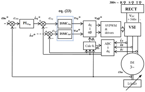
Finally, the block diagram of the proposed control scheme is presented in Figure 1.
Figure 1.
Block diagram of the proposed scheme.
Remark 2.
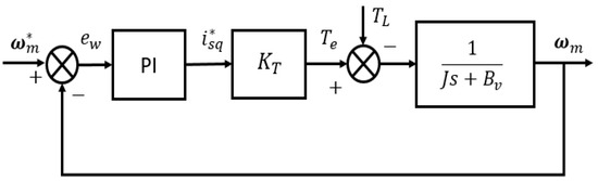
Assuming that the dynamics associated with the IM stator current controller blocks, the SVPWM and the VSI blocks are much faster in respect to the induction motor dynamics, they can be neglected [29]. Moreover, considering that the rotor flux current command, , is constant, so that we will get the simplified blocks diagram, which is shown in Figure 2. As indicated in the diagram, a PI regulator has been used to control the mechanical speed of the machine, implying that this regulator must be adjusted to get the faster dynamics as it is possible. The frequency-domain method is used to get the speed regulator’s adjusted parameters while stability being guaranteed [29].
Figure 2.
Simplified block diagram of the IM speed regulation.
4. Simulation and Experimental Results
In this section, the performance of the proposed current regulations has been verified in the MATLAB/Simulink environment and in the real tests by using a commercial induction motor.
The experimental validation of the proposed ISMC regulators has been carried out by using the control platform shown in Figure 3 and Figure 4.
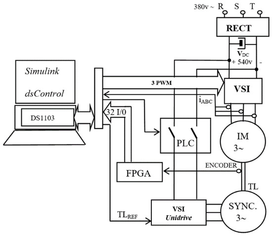
Figure 3.
The Blocks diagram of the IM experimental platform.
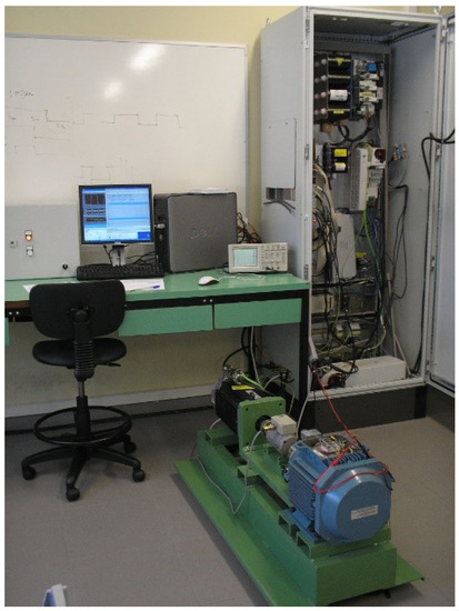
Figure 4.
The experiment platform for IM with load.
The design block consists of a personal computer with the Windows XP operating system where MATLAB/Simulink from MathWorks, dSControl from dSPACE, and the real-time interface from dSpace are installed. This interface allows the user to run in real-time the designs that are made in Simulink through MATLAB’s Real-Time Workshop.
The card is a powerful real-time interface that is connected in a portable slot of the PC and has a from Motorola at 1 GHz, a DSP that allows generating SVPWM in a very simple way, as well as 32 I/O pins, 8 D/A channels and 4 A/D channels, among the most important resources. The dSControl software, which connects to the board, is used to monitor on the PC the different signals and variables of the real tests that are executed on the motor platform. Thus, these signals can be compared with their counterparts obtained in Simulink and perform the appropriate validations.
The power block is composed of a DC bus, the inverters to control the two motors, and the bank composed of the two motors. The 540-V DC bus is obtained from a 380 V/50 Hz three-phase grid, by means of a semi-controlled rectifier and a 27-mF capacitor bank. The inverter for the induction motor is a 50-A industrial three-phase IGBT bridge, and the synchronous motor is an Emerson Unidrive programmable inverter. The IGBT bridge is used as a three-phase inverter to power the stator of the induction motor, which is controlled with the functions of the Simulink SVPWM library for . On the other hand, the synchronous motor has its own Unidrive inverter, which is torque controlled with a DC voltage set-point proportional to the torque to be generated, and which is sent from the .
As for the motor platform, it consists of a -kW three-phase induction motor from , on whose shaft is connected to a -kW Unimotor synchronous motor from Emerson, which is used to produce the load torque on the induction motor.
The control and monitoring tasks are done from a personal computer, which has installed the software MATLAB/Simulink and dSControl, and the controller board real-time interface of dSpace.
The mechanical speed of the machine is calculated by an FPGA module by using the measurements of an incremental encoder of 4096 impulses per revolution. The PLC is used to ensure that the basic operations as the charge of the DC bus, are done safely. The algorithms for the speed and currents control, the flux and torque estimators, the angle calculation, Park’s reference frame transformations, and the calculations of SVPWM, have been implemented by using a S-Function Builder Simulink’s block programmed in C language, providing a portable compact code for different processors. The stator windings of IM have been protected by limiting the electromagnetic torque current command to ±20 A. The nominal value of the rotor flux (0.903 Wb) is obtained by keeping the rotor flux current command value at the constant value, 8.026 A.
Table 1 shows the values of the ISMC current regulators’ parameters for three distinct design scenarios applied to the same induction motor. The nominal parameter values (Table 2) are used by the IM in the both ISMC regulators, D1 and D2 designs, while these controllers are tuned by using the T1 and T2 are shown in the second and third columns. In the fourth column, with the T3 tuning, the Ls factor of the motor changes, whereas the rest of the machine specs will remain as before.

Table 1.
The three turnings of the two ISMC regulators (D1 & D2 designs).
Table 2.
Parameters of the M2AA 132M4 ABB Induction Motor 7.5 [rpm] and 1445 [rpm].
Regarding the adjustment of the PI current regulators, which are going to be employed to compare with the ISMC current regulators, in both stator currents loop a 3000 rad/s bandwidth and a margin phase of have been used to adjust the PI regulators as (). In this sense, as the mechanical speed loop is slower than the stator current loops, the bandwidth of the PI speed regulator is chosen to be ten times smaller than the current regulator. The PI regulator has been tuned, taking a bandwidth of 300 rad/s and a margin phase of , ( and ) [29]. This way the fastest possible dynamics have been obtained for IM experimentally by applying PI regulators.
By using D2 design and T3 adjustment (D2-T3), another experiment is done which considers term of the IM is lower than the rated value (Table 2): (with ), to demonstrate the robustness despite the parametric uncertainties of the machine.
Figure 5 shows the machine’s performance when the simulation is running at 600 rpm of speed. The motor works with a square speed reference of 2 s period, and the load torque is applied to the system in two steps: 10 Nm at the starting point, plus 20 Nm after s. Moreover, the experiment is carried out by applying D2 to the platform and tuning the controllers by using T1 tuning values. The first graph (a) depicts the reference and real rotor velocity, and the second graph (b), demonstrates the speed error.
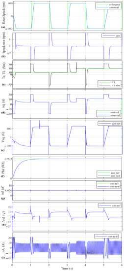
Figure 5.
Simulation results with 600 rpm reference speed and two load torque step changes (ISMC D2-T1): (a) Rotor speed, (b) Speed error, (c) , (d) Torque current, (e) , (f) Rotor flux, (g) Rotor flux current, (h) and (i) Stator current.
As can be seen, by a sudden change of the load torque, the rotor velocity tracks the speed reference properly, with less than 1 rpm error in steady state. This precise speed tracking is happening due to the good adjustment of the PI speed controller. The third graph (c), shows the electromagnetic torque and load torque, in which the smoothness of the electromagnetic torque is noticeable. In graph (d), it can be seen that the real torque current follows its reference properly, meaning that its error is minimum. Moreover, this current is limited to its maximum value (20 A), and it is proportional to the electromagnetic torque, which consequently is also smooth. The good quality of and is due to the fact that the output voltage of the regulator is also smooth and effective, which is obvious in the graph (e). In the (f) graph, it can be seen that rotor flux reaches and keeps its nominal value after s, and this is possible due to the precise rotor flux current tracking, as has been shown in the (g) graph. This is a consequence due to the output voltage of regulator. The efficiency of this signal is illustrated in the (h) graph. It can be observed that these two stator currents are decoupled. Finally, in graph (i), it can be observed that the stator currents are limited to the same value to which the torque current is bound.
Figure 6 depicts the machine performance by using the experimental test that corresponds to the simulation test presented in Figure 5. The speed tracking and accuracy are quite close to the simulation example, and it has fast dynamics, as shown in graphs (a) and (b). In steady state, speed error is less than 1 rpm, implying good accuracy in the presence of load disturbance. By comparing the electromagnetic torque (c) its simulation scenario, it is noticeable that both are fairly comparable, smooth, and efficient. Graph (d) shows that the torque current tracking is occurring precisely, and it is very similar to the simulation case, which is obtained due to the smooth and effective output voltage of its regulator, (e) graph. It has been demonstrated that the rotor flux (f), its related current (g), and the regulator’s output voltage (h) are very similar to their respective simulation ones. Finally, one phase of the stator currents is shown in graph (i). It is worth noting that the experimental voltages () and currents () have higher control action than the simulation case due to the unmodeled dynamics of the plant.
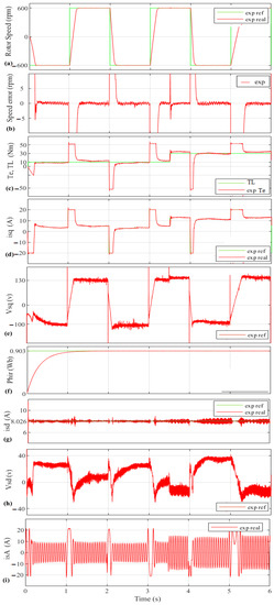
Figure 6.
Experimental results with 600 rpm reference speed and two load torque step changes (ISMC D2-T1): (a) Rotor speed, (b) Speed error, (c) , (d) Torque current, (e) , (f) Rotor flux, (g) Rotor flux current, (h) and (i) Stator current.
When comparing Figure 5 and Figure 6, it can be noted that the simulation and the experiment platform have almost identical behavior, indicating that the enhanced D2 design of ISMC stator currents regulators have been experimentally validated and have proper system modeling. An error and its integral signal are used in the conventional D1 design of ISMC technique to design the surface. Enhanced D2 design, on the other hand, uses the method to enhance the sliding surface (Equation (15)). In addition, to decrease chattering, the conventional D1 design ISMC’s function is substituted with one of its continuous approximation functions, such as (Equation (23)).
5. Results Discussion
In this section, the capability of the proposed controller in comparison with two other control techniques, PI controller, and conventional ISMC, is demonstrated experimentally.
In this regard, Figure 7 shows a comparison of the D1 (conventional method) and D2 (proposed method) controllers. These tests have the same speed and load conditions as Figure 6. For extracting Figure 6, experiments have been done in three stages: first, T1 tuning is considered for D1 (D1-T1). Moreover, D2 is tuned by using T1 tuning (D2-T1). Finally, to have a better tune for D1 in order to get best dynamics of the whole system, T2 values are taken (D1-T2). The enhanced controller’s current regulator output (), which is quicker and smoother than the two conventional versions, is shown in graph (a). The outcome of the D1-T1, is slower, more aggressive, and has a higher current error (b) than the D2-T1 case. As a consequence, the electromagnetic torque of the D1-T1 is slower and more aggressive than the D2-T1 case. By applying the D1-T2, the output of the controller is faster but more aggressive than the D1-T1, but still slower than the D2-T1. As a result, its electromagnetic torque is faster and more aggressive than the D1-T1 gains, generating chattering and slower than the D2-T1, graph (c).
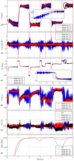
Figure 7.
Experimental tests for and performance comparison between the enhanced ISMC D2 design and the conventional ISMC D1 design with 600 rpm reference speed: (a) , (b) error, (c) , (d) , (e) and (f) Rotor flux.
On the other hand, graph (d) shows the comparison between current regulator output () for both conventional and enhanced methods. As can be observed, D1-T1 causes the machine to lose control at some instances (graphs (e) and (f)). The conventional technique requires the use of T2 design values in this circumstance. The output of the conventional current regulator () has a certain amount of fluctuation, as can be seen in the (d) graph, but the enhanced controller still gives a superior signal for and flux ((e) and (f) graphs).
The graphs of Figure 8 and Figure 9 show the comparison of the experimental tests between the enhanced ISMC (D2-T1) and the PI current regulators by using the same speed and load conditions as in the test of Figure 5. For running these experiments, once the PI controllers have been adjusted without considering and coupling terms of currents (Feed-Forward, FF) action and once by considering FF action, which means PI regulators are running at their best adjustment condition. As has been shown in the (a) graph of Figure 8, the response is slightly smoother by using the enhanced ISMC D2 regulator in comparison to two PI controllers. Moreover, the error can be observed in the (b) graph indicates that by using the PI controller without FF, the motor is losing control at some instants (1 s, 2 s, 3 s).
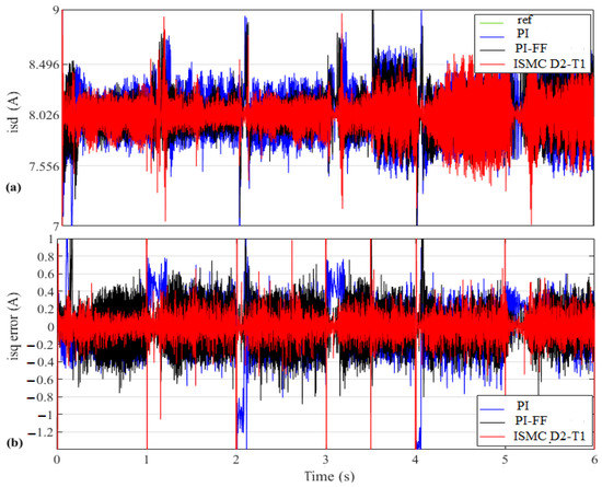
Figure 8.
Experimental tests for and performance comparison between the enhanced ISMC D2 design and the PI regulators with 600-rpm reference speed: (a) and (b) error.
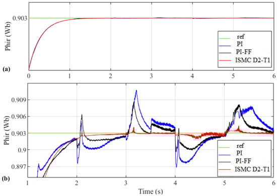
Figure 9.
Experimental tests for flux performance comparison between the enhanced ISMC D2 design and the PI regulators using 600-rpm reference speed: (a) Rotor flux and (b) Magnification of the rotor flux.
Furthermore, by applying the ISMC regulator, the error bound is notoriously lower compared to the case in which the motor is running by PI stator current controllers. Hence, the performance of the presented regulator is better than PI.
Experiments for flux performance comparison between the enhanced ISMC D2 and the PI regulators are shown in Figure 9. The ISMC regulator is correcting the effect of the current coupling terms in graph (b). As a consequence, it is getting good control over the rotor flux, whereas by using the PI regulator, the compensation is worse and the rotor flux control is not so good (losing the flux tracking at the 1 s, 2 s, 3 s, 4 s, and 5 s instants). This performance leads us to take advantage of the flux-weakening regimen, which demands high precision in the rotor flux.
The outcomes of the experimental comparisons between the proposed method and the existing ones are provided in Table 3.
Table 3.
Comparison of the proposed method vs two other existing methods.
Figure 10 shows the experimental test in which the maximum value of the reference speed is 2000 rpm, which is higher than the rated value of the motor (1445 rpm, Table 2), whereas the rotor flux is lower than the rated value. This way, the machine works in a rotor flux-weakening regimen. In this experiment, the following load disturbance is applied to the regulated motor by enhanced ISMC D2 design: = 10 Nm at t = 0 s, and 7 Nm after s is added to the initial value. It can be seen that speed tracking (a) is extremely good, with an outstanding accuracy of 3 rpm of error steady-state (b). The electromagnetic torque is smooth and effective (c), with no chattering, beccause the torque current tracking is excellent (d). The rotor flux for this regimen achieves and maintains a tight, constant value of 0.5872 Wb, as shown in graph (e). This is made feasible by a precise rotor flux regulation (f), which keeps the actual current at the same level as its reference, 5.22 A. Finally, the (g) graph shows the A stator current, which shows that the three-phase currents are limited to approximately 20 A to protect the stator winding from over-currents.
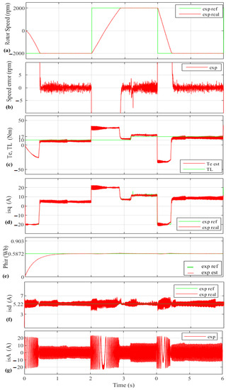
Figure 10.
Experimental results using 2000-rpm reference speed and two load torque step changes (enhanced ISMC D2 design): (a) Rotor speed, (b) Speed error, (c) , (d) Torque current, (e) Rotor flux, (f) Rotor flux current and (g) Stator current.
Figure 11 shows the simulation performance of the machine by using enhanced ISMC D2 design with T3 tuning, which employs a theoretical machine with a lower factor (by taking a lower ). The machine has been tested by employing a medium-high speed test (1200 rpm), and it can be observed that speed tracking, graphs (a) and (b), and also the rotor flux tracking, graph (c), are excellent. Moreover, both tracking of stator currents are also good, as seen in graphs (d) and (e).
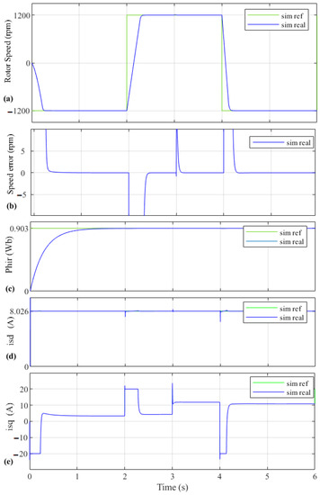
Figure 11.
Simulation results with 1200-rpm reference speed and two load torque step changes, with higher uncertainty in (enhanced ISMC D2 design T3 tuning): (a) Rotor speed, (b) Speed error, (c) Rotor flux, (d) Rotor flux current and (e) Torque current.
The outcome of experimental performance, which corresponds to the simulation presented in Figure 11, is shown in Figure 12. However, it is important to note that the value of factor in the real machine employed in this experiment is 60% higher than the ISMC D2 design T3 tuning case. Graphs (a) and (b) show that the speed tracking and the speed error (minor than 2 rpm) are very satisfactory. Furthermore, rotor flux has good tracking, reaching, and maintaining the rated imposed value consistently, as shown in graph (c). These good accuracy is the result of proper tracking in both stator currents, graphs (d) and (e), which present highly satisfactory and resilient tracking in the presence of significant parameter uncertainties.
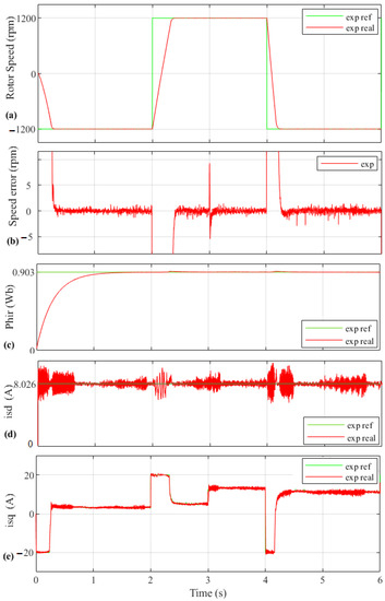
Figure 12.
Experimental results with 1200-rpm reference speed and two load torque step changes, with higher uncertainty in (enhanced ISMC D2 design T3 tuning): (a) Rotor speed, (b) Speed error, (c) Rotor flux, (d) Rotor flux current and (e) Torque current.
6. Conclusions
In this paper, the ISMC method is applied to the IM vector control system. The purpose is to regulate the d-q stator current components and reject their coupling term disturbances and parameter uncertainties. The proposed controllers incorporate an integral part in the sliding surface to eliminate static machine errors and enhance the regulator accuracy. Moreover, the stability analysis of the controllers has been done based on the Lyapunov function approach. The simulation and experimental tests employing a commercial IM have confirmed their experimental validation. It has been demonstrated that in the experiment platform, the proposed controllers have more robust, chattering-free, and fast performance in comparison with the classical PI current controllers and the conventional ISMC method. Also, the output of this achievement is an effective, quick, smooth, and chattering-free electromagnetic torque. Furthermore, the enhanced current controllers provide effective results in the rotor flux weakening regimen. Finally, the regulators’ ability to eliminate system chattering under significant stator electrical uncertainty and current coupling disturbances demonstrates the controlled system’s reliability.
Author Contributions
Conceptualization, F.S., P.A., J.A.C. and O.B.; methodology, F.S. and P.A.; software, F.S., P.A. and J.A.C.; validation, F.S., P.A. and J.A.C.; formal analysis, O.B.; investigation, F.S. and P.A.; resources, O.B.; data curation, P.A.; writing—original draft preparation, F.S.; writing—review and editing, F.S., P.A., J.A.C. and O.B.; visualization, J.A.C. and O.B.; supervision, P.A. All authors have read and agreed to the published version of the manuscript.
Funding
The University of the Basque Country (UPV/EHU) [grant number PIF 18/127] has funded the research in this paper.
Acknowledgments
The authors wish to express their gratitude to the Gipuzkoako Foru Aldundia through the project Etorkizuna Eraikiz 2022–2023, the Basque Government through the project EKOHEGAZ (ELKARTEK KK-2021/00092), the Diputacion Foral de Alava (DFA) through the project CONAVANTER, and to the UPV/EHU through the project GIU20/063 for supporting this work.
Conflicts of Interest
The authors declare no conflict of interest.
Nomenclature
| Symbols of Induction Motor | |
| Viscous friction coefficient | |
| J | Moment of inertia |
| Magnetizing inductance | |
| Stator inductance | |
| Rotor inductance | |
| Rotor resistance | |
| Stator resistance | |
| p | Number of poles |
| Coefficient of magnetic dispersion | |
| Electromagnetic torque | |
| Load or disturbance torque | |
| Mechanical rotor speed | |
| Mechanical rotor reference speed | |
| Synchronous speed | |
| Rotor flux | |
| I | Stator rated current |
References
- Liu, X.; Yu, H.; Yu, J.; Zhao, L. Combined speed and current terminal sliding mode control with nonlinear disturbance observer for PMSM drive. IEEE Access 2018, 6, 29594–29601. [Google Scholar] [CrossRef]
- Bensalem, Y.; Abbassi, A.; Abbassi, R.; Jerbi, H.; Alturki, M.; Albaker, A.; Abdelkrim, A.; Kouzou, A.; Abdelkrim, M.N. Speed tracking control design of a five-phase PMSM-based electric vehicle: A backstepping active fault-tolerant approach. Electr. Eng. 2022, 104, 2155–2171. [Google Scholar] [CrossRef]
- Lin, C.H.; Ting, J.C. Novel nonlinear backstepping control of synchronous reluctance motor drive system for position tracking of periodic reference inputs with torque ripple consideration. Int. J. Control. Autom. Syst. 2019, 17, 1–17. [Google Scholar] [CrossRef]
- Diab, A.A.Z.; Elsawy, M.A.; Denis, K.A.; Alkhalaf, S.; Ali, Z.M. Artificial Neural Based Speed and Flux Estimators for Induction Machine Drives with Matlab/Simulink. Mathematics 2022, 10, 1348. [Google Scholar] [CrossRef]
- Sabzalian, M.H.; Alattas, K.A.; El-Sousy, F.F.; Mohammadzadeh, A.; Mobayen, S.; Vu, M.T.; Aredes, M. A Neural Controller for Induction Motors: Fractional-Order Stability Analysis and Online Learning Algorithm. Mathematics 2022, 10, 1003. [Google Scholar] [CrossRef]
- Li, C.; Wang, Z.S.; Tian, Y.F. Dynamic event-triggered H∞ load frequency control for multi-area power systems with communication delays. Int. J. Robust Nonlinear Control 2021, 31, 4100–4117. [Google Scholar] [CrossRef]
- Ramya, L.; Sivaprakasam, A. Application of model predictive control for reduced torque ripple in orthopaedic drilling using permanent magnet synchronous motor drive. Electr. Eng. 2020, 102, 1469–1482. [Google Scholar] [CrossRef]
- Chen, J.; Huang, J. Application of adaptive observer to sensorless induction motor via parameter-dependent transformation. IEEE Trans. Control Syst. Technol. 2018, 27, 2630–2637. [Google Scholar] [CrossRef]
- Sun, Y.; Yan, S.; Cai, B.; Wu, Y.; Zhang, Z. MPPT Adaptive Controller of DC-based DFIG in Resistances Uncertainty. Int. J. Control Autom. Syst. 2021, 19, 2734–2746. [Google Scholar] [CrossRef]
- Ge, Y.; Yang, L.; Ma, X. Adaptive sliding mode control based on a combined state/disturbance observer for the disturbance rejection control of PMSM. Electr. Eng. 2020, 102, 1863–1879. [Google Scholar] [CrossRef]
- Sumbekov, S.; Phuc, B.D.H.; Do, T.D. Takagi–Sugeno fuzzy-based integral sliding mode control for wind energy conversion systems with disturbance observer. Electr. Eng. 2020, 102, 1141–1151. [Google Scholar] [CrossRef]
- Shiravani, F.; Alkorta, P.; Cortajarena, J.A.; Barambones, O. An Enhanced Sliding Mode Speed Control for Induction Motor Drives. Actuators 2022, 11, 18. [Google Scholar] [CrossRef]
- Du, C.; Yang, C.; Li, F.; Gui, W. A novel asynchronous control for artificial delayed Markovian jump systems via output feedback sliding mode approach. IEEE Trans. Syst. Man Cybern. Syst. 2018, 49, 364–374. [Google Scholar] [CrossRef]
- Mishra, J.; Wang, L.; Zhu, Y.; Yu, X.; Jalili, M. A novel mixed cascade finite-time switching control design for induction motor. IEEE Trans. Ind. Electron. 2018, 66, 1172–1181. [Google Scholar] [CrossRef]
- Utkin, V.I. Sliding mode control design principles and applications to electric drives. IEEE Trans. Ind. Electron. 1993, 40, 23–36. [Google Scholar] [CrossRef] [Green Version]
- Sabanovic, A.; Izosimov, D.B. Application of sliding modes to induction motor control. IEEE Trans. Ind. Appl. 1981, IA-17, 41–49. [Google Scholar] [CrossRef]
- Morawiec, M.; Lewicki, A.; Wilczyński, F. Speed observer of induction machine based on backstepping and sliding mode for low-speed operation. Asian J. Control 2021, 23, 636–647. [Google Scholar] [CrossRef]
- Horch, M.; Boumédiène, A.; Baghli, L. Backstepping approach for nonlinear super twisting sliding mode control of an induction motor. In Proceedings of the 2015 3rd International Conference on Control, Engineering & Information Technology (CEIT), Tlemcen, Algeria, 25–27 May 2015; pp. 1–6. [Google Scholar]
- Wu, S.; Zhang, J. A terminal sliding mode observer based robust backstepping sensorless speed control for interior permanent magnet synchronous motor. Int. J. Control Autom. Syst. 2018, 16, 2743–2753. [Google Scholar] [CrossRef]
- Saghafinia, A.; Ping, H.W.; Uddin, M.N.; Gaeid, K.S. Adaptive fuzzy sliding-mode control into chattering-free IM drive. IEEE Trans. Ind. Appl. 2014, 51, 692–701. [Google Scholar] [CrossRef]
- Oliveira, C.M.; Aguiar, M.L.; Monteiro, J.R.; Pereira, W.C.; Paula, G.T.; Almeida, T.E. Vector control of induction motor using an integral sliding mode controller with anti-windup. J. Control Autom. Electr. Syst. 2016, 27, 169–178. [Google Scholar] [CrossRef]
- Barambones, O.; Garrido, A.; Maseda, F. Integral sliding-mode controller for induction motor based on field-oriented control theory. IET Control Theory Appl. 2007, 1, 786–794. [Google Scholar] [CrossRef]
- Tak, R.; Kumar, S.Y.; Rajpurohit, B.S. Estimation of Rotor and Stator Resistance for Induction Motor Drives using Second order of Sliding Mode Controller. J. Eng. Sci. Technol. Rev. 2017, 10, 9–15. [Google Scholar] [CrossRef]
- Nollet, F.; Floquet, T.; Perruquetti, W. Observer-based second order sliding mode control laws for stepper motors. Control Eng. Pract. 2008, 16, 429–443. [Google Scholar] [CrossRef]
- Mousavi, M.S.; Davari, S.A.; Nekoukar, V.; Garcia, C.; Rodriguez, J. Integral sliding mode observer-based ultra-local model for finite-set model predictive current control of induction motor. IEEE J. Emerg. Sel. Top. Power Electron. 2021, 10, 2912–2922. [Google Scholar] [CrossRef]
- Rai, R.; Shukla, S.; Singh, B. Sensorless field oriented SMCC based integral sliding mode for solar PV based induction motor drive for water pumping. IEEE Trans. Ind. Appl. 2020, 56, 5056–5064. [Google Scholar] [CrossRef]
- Gou, L.; Wang, C.; Zhou, M.; You, X. Integral sliding mode control for starting speed sensorless controlled induction motor in the rotating condition. IEEE Trans. Power Electron. 2019, 35, 4105–4116. [Google Scholar] [CrossRef]
- Comanescu, M. An induction-motor speed estimator based on integral sliding-mode current control. IEEE Trans. Ind. Electron. 2009, 56, 3414–3423. [Google Scholar] [CrossRef]
- Mohan, N. Advanced Electric Drives: Analysis, Control, and Modeling Using MATLAB/Simulink; John Wiley & Sons: Hoboken, NJ, USA, 2014. [Google Scholar]
- Jin, N.; Wang, X.; Wu, X. Current sliding mode control with a load sliding mode observer for permanent magnet synchronous machines. J. Power Electron. 2014, 14, 105–114. [Google Scholar] [CrossRef]
- Slotine, J.J.E.; Li, W. Applied Nonlinear Control; Prentice Hall: Englewood Cliffs, NJ, USA, 1991. [Google Scholar]
- Khalil, H.K. Nonlinear Control; Pearson: New York, NY, USA, 2015. [Google Scholar]
Publisher’s Note: MDPI stays neutral with regard to jurisdictional claims in published maps and institutional affiliations. |
© 2022 by the authors. Licensee MDPI, Basel, Switzerland. This article is an open access article distributed under the terms and conditions of the Creative Commons Attribution (CC BY) license (https://creativecommons.org/licenses/by/4.0/).