1. Introduction
Currently, there is a great interest in research on non-destructive (non-invasive) methods for the detection of sources or unknown characteristic(s) of a system from partial information on the mentioned system [
1,
2]. Examples of this are medical tomography, industrial process tomography, inverse geophysics, inverse electroencephalography, and inverse electrocardiography [
3,
4,
5,
6,
7,
8,
9].
In medical tomography, the objective is to identify a bioelectric source from one or more external manifestation effects produced by that source and measured by means of an electronic device. Non-invasive techniques include magnetic resonance and radio-isotope imaging, which provide functional images of blood flow and metabolism, essential for diagnosing and investigating the brain, heart, liver, kidney, bones, and other organs of the human body. One non-invasive technique for the reconstruction of brain or cardiac electrical activity from electrical potentials measured outside the brain, using electroencephalograms (EEG), and the heart, using electrocardiograms (ECG), is the so-called electrical source imaging, which consists of “reconstructing” the brain or heart activity from potentials measured outside the brain or heart. This method is used in electrocardiography or electroencephalography to determine the location of current sources in the body or brain from voltage measurements; it is also used for diagnosis and therapeutic guidance regarding epilepsy and abnormalities in the conduction of the heart. These last two methods for source identification from measurements at the boundary of a conductive medium are known as the electrocardiographic inverse problem and electroencephalographic inverse problem (we will abbreviate the latter as EIP). In particular, the EIP consists of finding bioelectric sources (which are generated by the electrochemical activity of large conglomerates of neurons that act simultaneously) in the brain from the EEG measured on the scalp. One of the advantages of the EEG is that the information it provides is captured in real-time, in a simple way, and it is non-invasive as well as inexpensive. On the other hand, the EIP is an ill-posed problem because there is a diversity of sources that produce the same measurement, and it is impossible to univocally determine the source that generated the EEG; that is, there is more than one source that can produce or generate the same EEG [
10,
11]. The ill-posedness of this problem is also associated with numerical instability, i.e., small variations in the EEG can produce substantial variations in the location of the source [
5]. In general, sources cannot be determined except for their harmonic component [
12,
13]. In [
13,
14], a stable algorithm is presented to identify the harmonic component of the source from noisy data, when the head is modelled by concentric circles or concentric spheres. To find the non-harmonic component of the source, it is necessary to have a priori information, which can be determined from mathematical or physiological considerations [
10,
12,
15,
16]. In particular, in [
16] the fact that the unknown source belongs to a class of piecewise constant functions is considered a priori information, and the uniqueness of the solution to the inverse problem is proved. Furthermore, the authors presented a stable method to identify an approximate solution within this class of sources when the data includes measurements errors. The method was illustrated in simple geometries.
In this work, a methodology is proposed to recover the complete source in a stable form, in circular and irregular geometries. We employ a variational formulation and distributed control techniques to obtain a numerical method which allows us to find solutions to the inverse source identification problem in a stable way. In the first step, the numerical method allows us to obtain harmonic sources in the interior of a non-homogeneous region (made of two or three conductive layers with constant and positive conductivity in each layer) from noisy measurements on the exterior boundary. The methodology combines conjugate gradient iterations (CG) to find the optimal control and finite element approximations (FE) for the elliptical problems that appear in each iteration of the CG. This methodology has already been used by other authors to solve inverse and control problems in other contexts (see [
17,
18,
19]). The second step consists of recovering the non-harmonic component of the source, taking into account a priori information. We apply the mentioned methodology to 2D synthetic examples, defined in a simple circular domain and in irregular complex regions. The proposed algorithm may be applied and implemented for the identification of 3D bioelectric sources in the brain from the EEG measured on the scalp, which is the object of future study.
The organization of this work is as follows.
Section 2 introduces a mathematical model from where the operational statement of the inverse source problem is established. In
Section 3, the variational formulation of the inverse problem is presented as a control problem. Additionally, the derivative of the cost function
is presented, and the optimality conditions of the minimization problem are established. In
Section 4, the CG algorithm is presented in detail, as well as the discretization of the elliptical problems using FE. We also include the analytical solutions to the forward and inverse problems in a circular geometry when the region is made of two and three conducting layers. In
Section 5, some numerical results are presented to recover harmonic functions defined in the interior region. These examples are developed in a circular and irregular two-dimensional region made of two or three conductive layers.
Section 6 presents three examples for which we compute the non-harmonic component of the complete source, besides its harmonic component and the complete source using a priori information. Finally, in
Section 7, some conclusions are established.
5. Numerical Results for Harmonic Sources
In this Section, we present numerical results when the volumetric source to be identified is harmonic. The examples presented in this section are designed to test the numerical algorithm introduced in
Section 4. Numerical examples for the general case (non-harmonic) will be presented in the next section.
For each example, we generate synthetic data V in either a simple domain or an irregular domain made of either two or three layers. To generate this data, we solve the state equation to obtain the exact potential u from a known harmonic source , and then we get (forward problem). Then, we solve the inverse problem with the numerical algorithm using V as input data to the control problem (20). The numerical recovered source will be denoted by , where h is the mesh size, n is the number of conjugate gradient iterations (cg. iters.) to achieve the desired accuracy (given by tolerance ), and is the regularization parameter obtained by the L-curve criterion. Similarly, the numerical potential obtained with this numerical source is denoted by .
Noisy data
with
are generated, adding to noiseless data
V ‘white noise’ with mean
and standard deviation
. Using the
function of MATLAB, we define the random vector
with length
the number of mesh nodes on the exterior boundary
. The corresponding approximate solutions are denoted by
and
. Of course,
is the regularization parameter that depends on the level of noise
(see
Section 2.2).
From now on, we will use the following notation for the relative errors:
For the computational implementation, the elliptic subproblems, at each step of the Algorithm 1, are solved using FE with linear triangular elements, so we generate an initial mesh called with mesh size , where indicates the number of nodes (vertices) and denotes the number of elements (triangles). Successive regular refinements will be denoted by for .
Example 1. We present a case with a simple circular domain made of two and three layers and a harmonic source. We consider a circular region Ω, which is made of either two or three circular layers. For the first case, is determined by two concentric circles with circumferences and of radii and , and constant conductivities and , respectively. For the second case, is determined by three concentric circles with circumferences , , and of radii , , and , and constant conductivities , , and , respectively. In both cases, for the harmonic source in these examples, we choose the exact function with , which in Cartesian coordinates is , . For the second case, the exact potential can be computed with Formulas (54)–(56), and its value on the exterior boundary V is generated by (57). Observe that only the second mode survives in the expansion of each Fourier series. After computing the Fourier coefficients and transforming them to Cartesian coordinates, we obtain (for the case of the domain Ω with three layers):where the values of the coefficients , , , , , are obtained using the expressions given in Section 4.2, and the values of parameters , , , , and are given above in this Section. Similar solutions in , in , and V on are obtained for the case of the domain with two layers.
Case with exact data. We assume that measurement
V on
is noiseless. The solution to the inverse problem is achieved with the regularization parameter
and tolerance
(for the stopping criterion of the Algorithm 1).
Table 1 shows that the relative errors decrease with each refinement of the coarse mesh
. These results show numerical convergence regarding the finite element discretization. Additionally, the accuracy of the solution in this case is very good for both the two and three coupled circular regions.
Case with noisy data. Here, we consider noisy data
on
with three different noise levels
. The coarsest mesh
is the same as before, and the numerical solutions are achieved with tolerance
to stop the conjugate gradient iterations and with the regularization parameters shown in
Table 2. This Table shows that the method to find the numerical solutions to the ill-posed inverse problem is stable. Actually,
and
are bounded by the perturbation
when
. Additionally, when noise vanishes, the numerical solution converges to the one obtained with noiseless data.
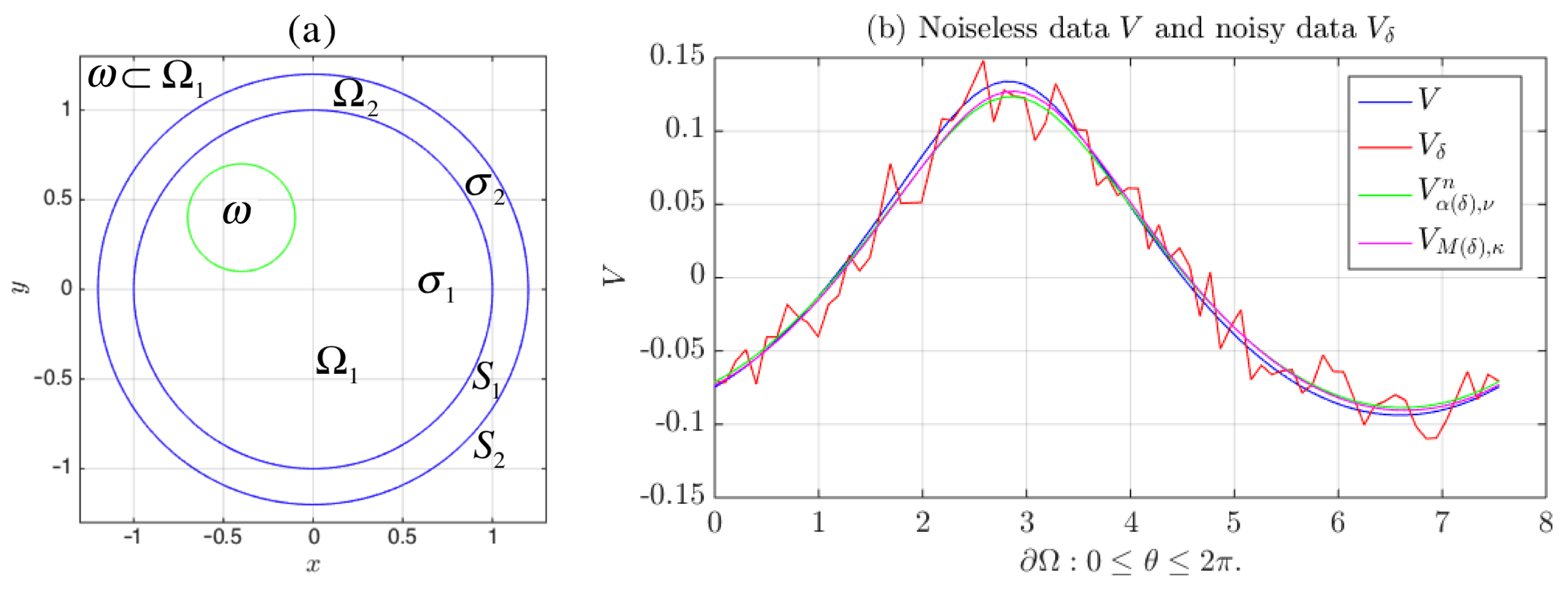
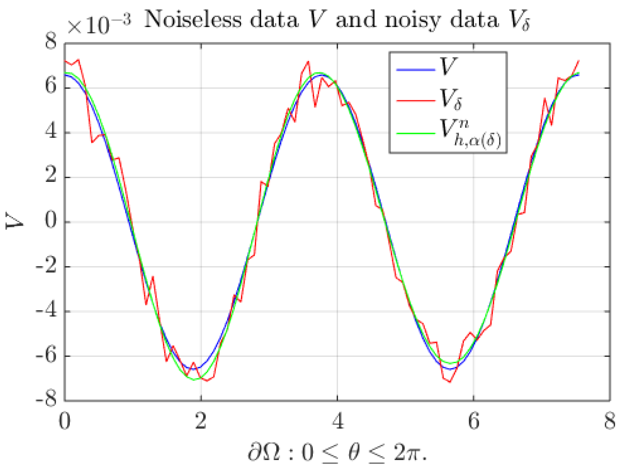
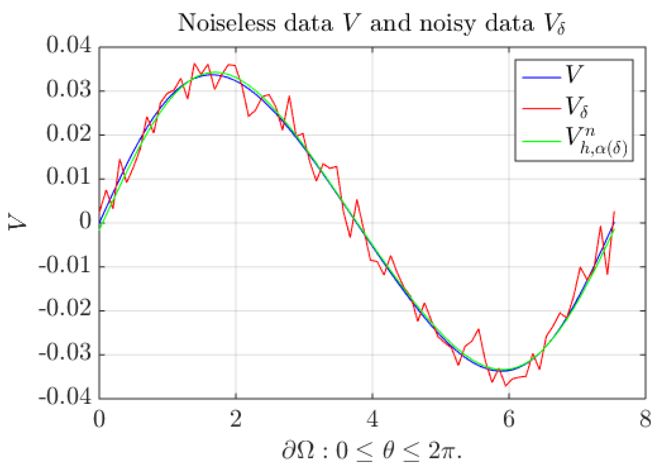
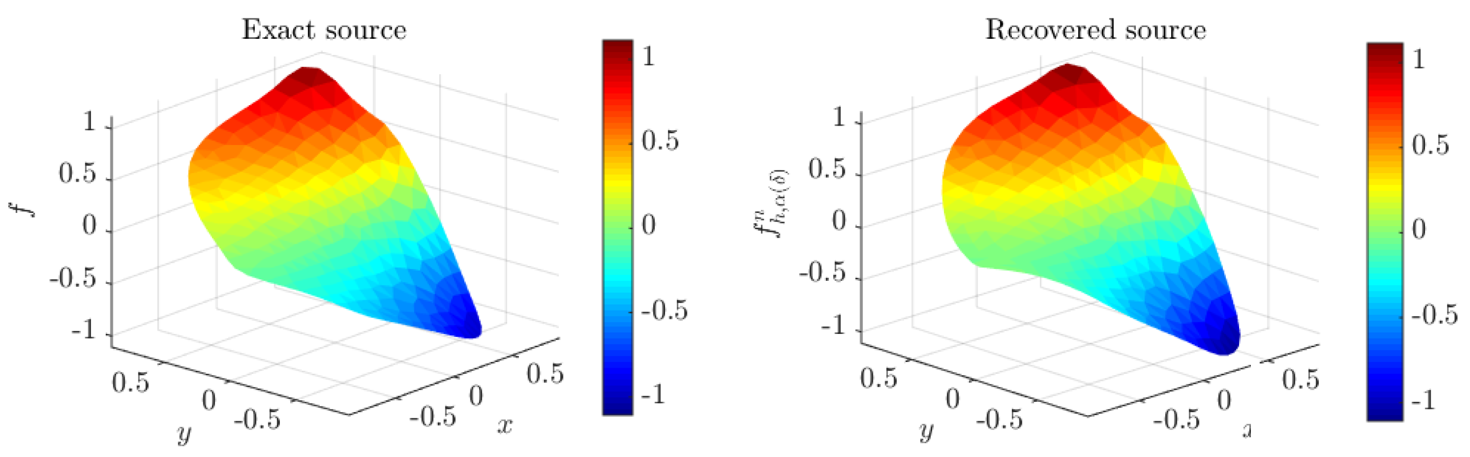
To better illustrate, below we include several figures which show plots of numerical results for the case of three circular coupled media and . The corresponding figures for two circular coupled media are qualitatively similar and are not included.
Figure 2 shows a plot of noisy data
along with exact data
V and the numerical external potential
obtained with the recovered source
.
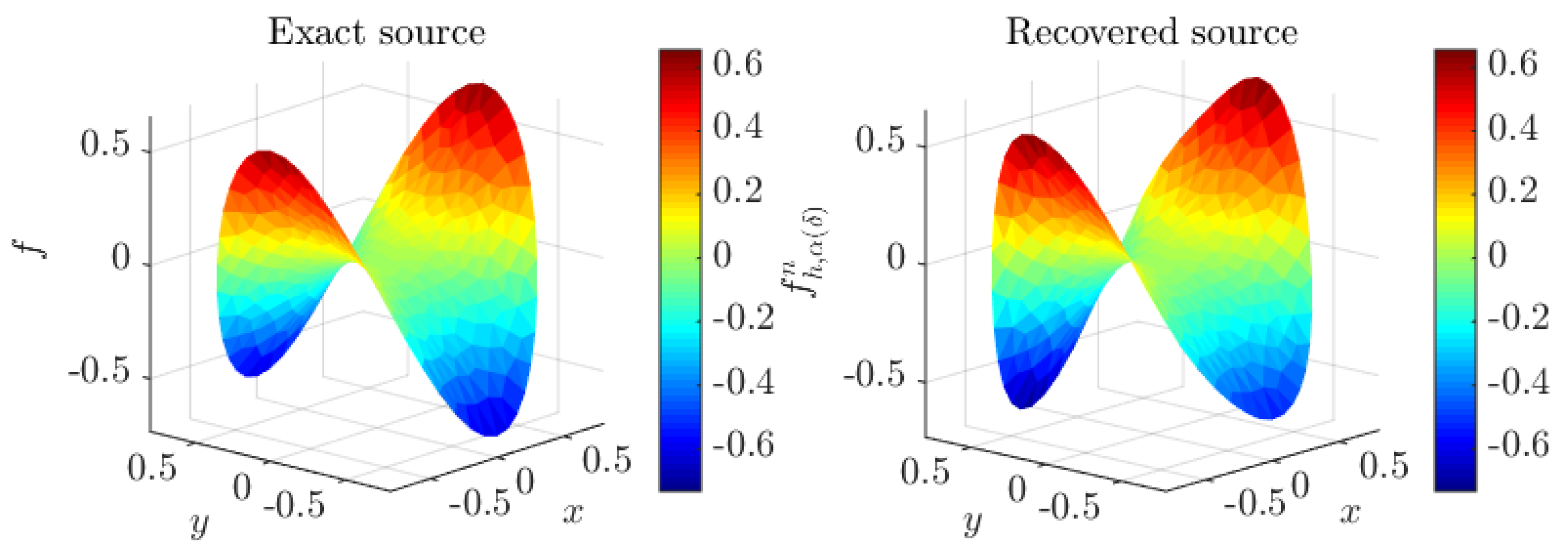
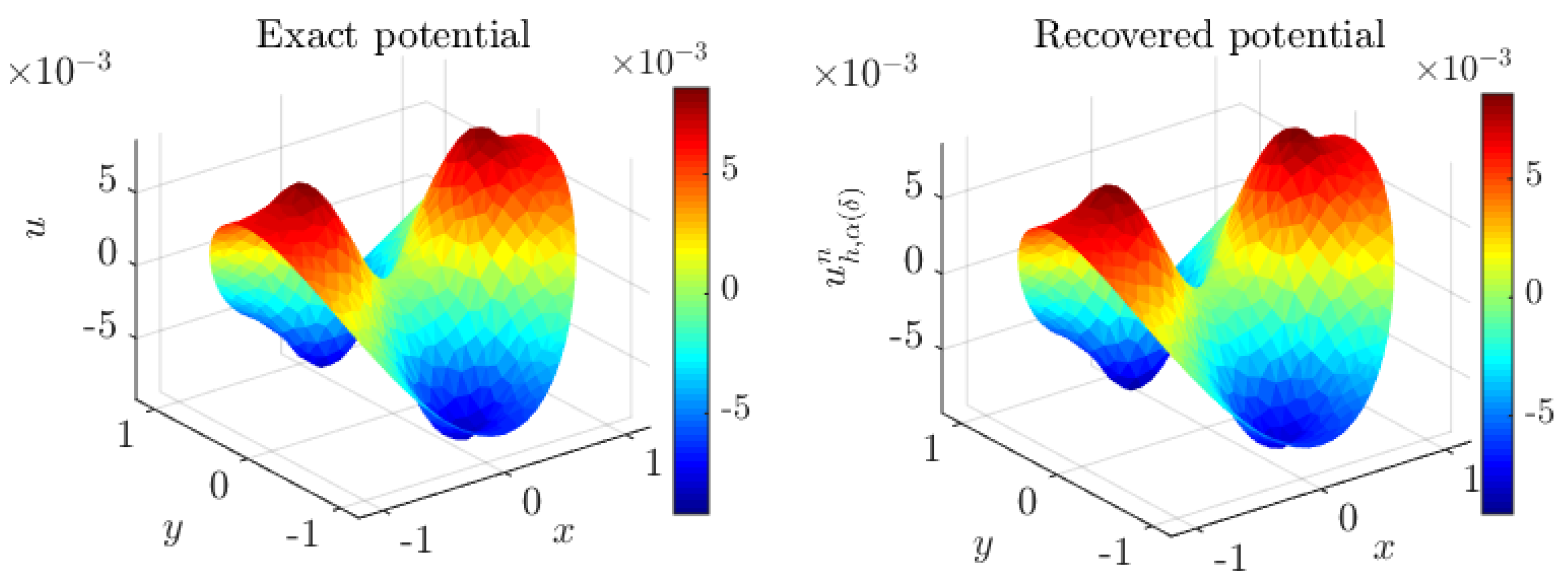
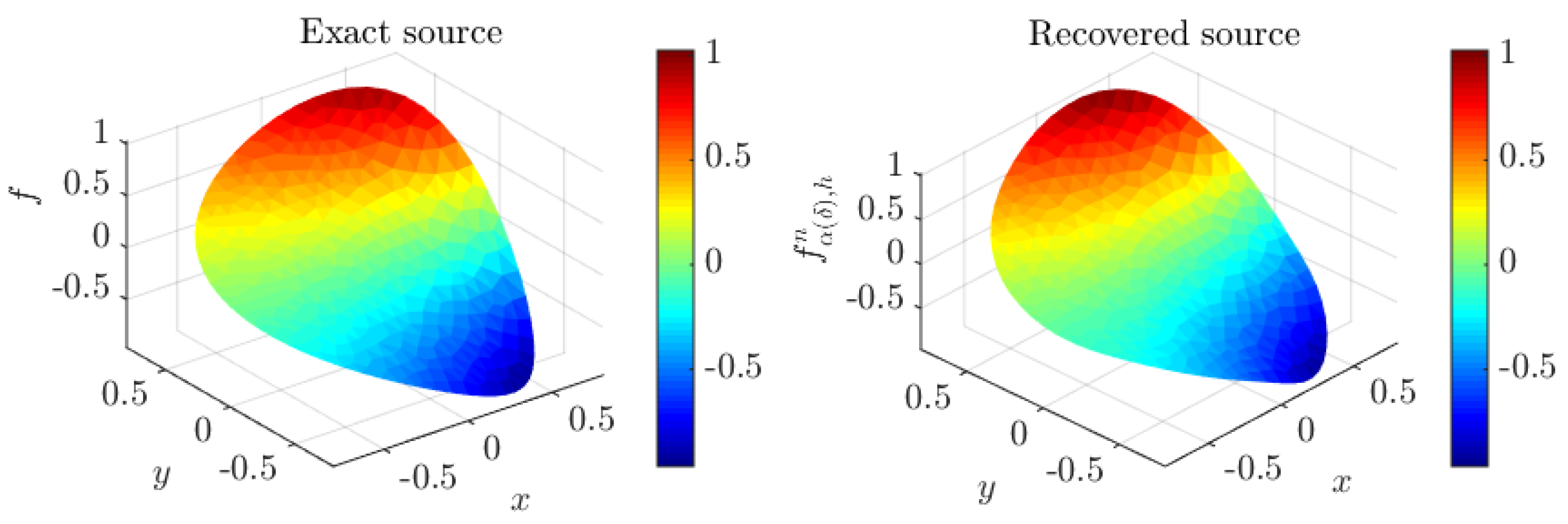
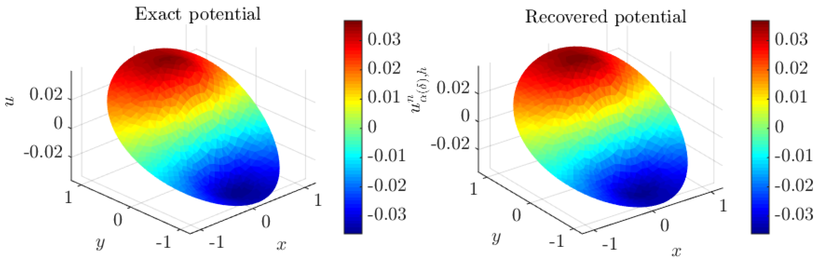
Figure 3 and
Figure 4 show plots of the numerical source
and the numerical potential
, respectively.
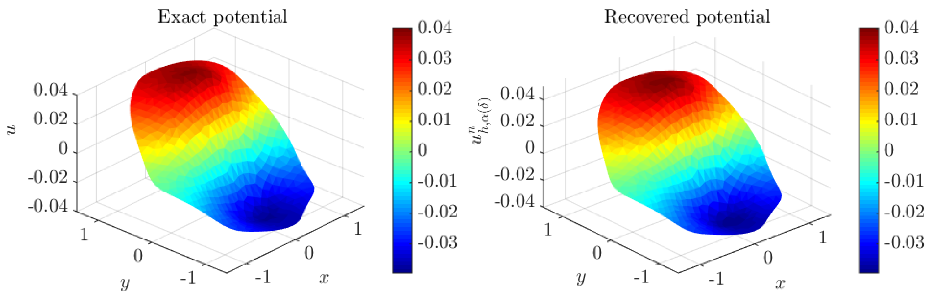
Example 2. We present here a case with a simple circular domain made of two and three layers and a harmonic source. For this example, we consider the harmonic source , , or, in polar coordinates, , . This function does not have a finite Fourier expansion, so it is approximated by a truncated series with N terms. The Fourier coefficients and , , are obtained numerically using the function quad2d of MATLAB. We choose , since for this value . Hereafter (in this example), we will call the exact source and will denote it as f. The exact solution u to the state Equations (7)–(14) is obtained with the first terms of series (54)–(56) for the domain with three circular coupled media. Similarly, exact data V are generated with the first terms of series (57). Synthetic data and the exact potential for the case when the domain is compound of two coupled media are obtained in the same way.
Case with exact data. Notice that data
V are not really exact, but they are an accurate approximation on
. The solution to the inverse problem is achieved with the regularization parameter
and tolerance
for the case of two conductive layers and
for three conductive layers, as shown in
Table 3. This Table shows that the numerical solutions are still accurate and convergent with respect to
h.
Case with noisy data.
Table 4 shows numerical results for different levels of noise for perturbed data
and a discretization obtained with mesh
. Again, the numerical results show the stability of the numerical method, and the relative errors are all bounded above by perturbation
when
.
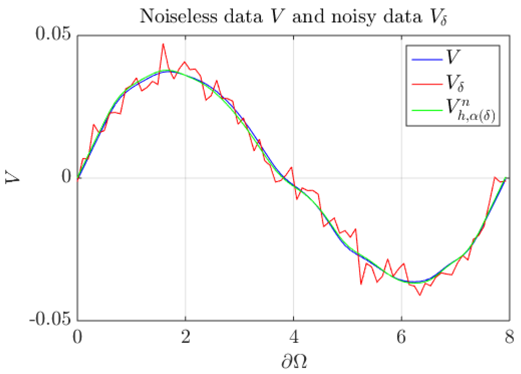
Again, below we include
Figure 5,
Figure 6 and
Figure 7 to compare the numerical solutions with the exact ones only for the case of the three circular coupled domain and when
.
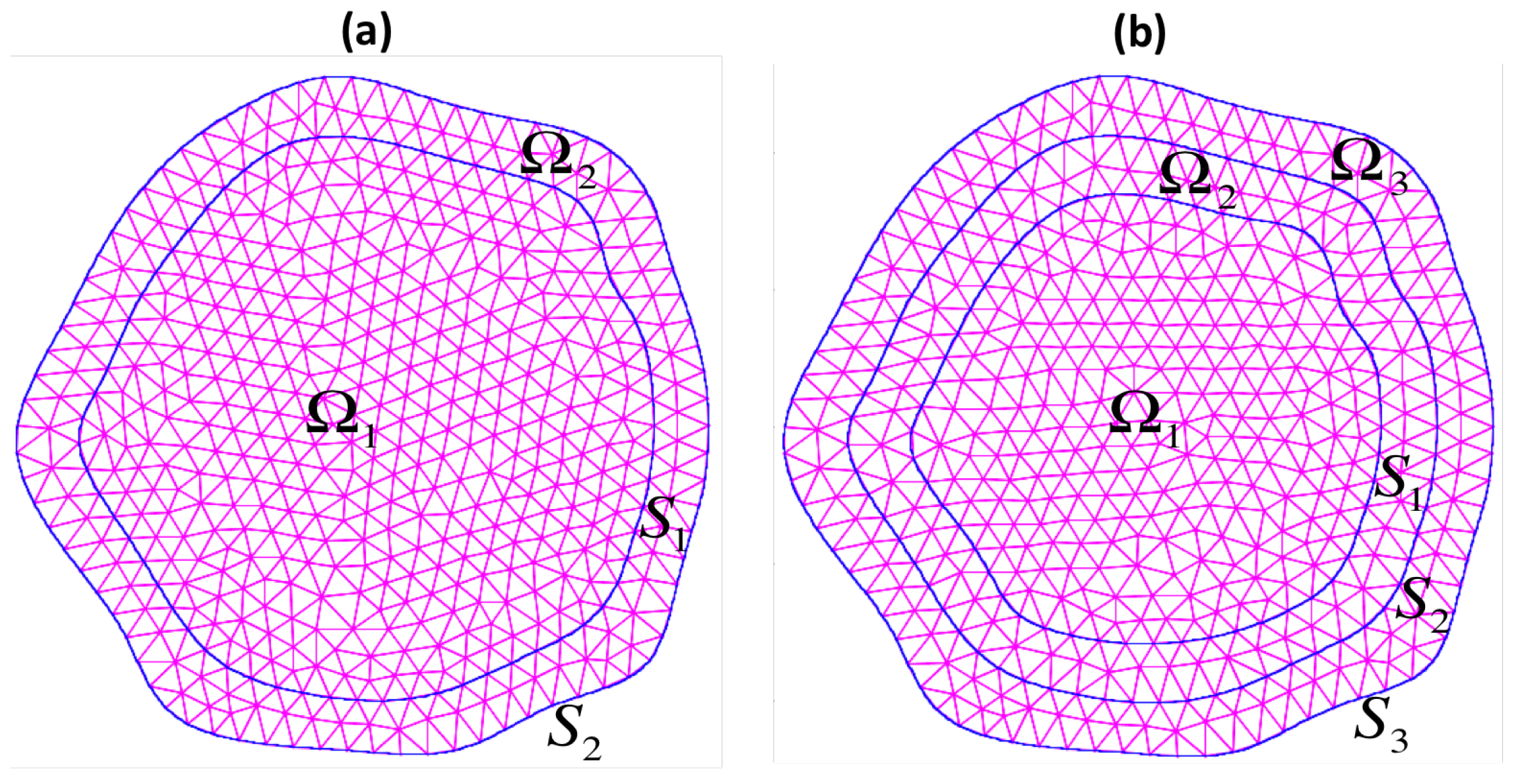
Example 3. Solution to the inverse problem in an irregular region. In this example, we consider the irregular regions shown in Figure 1. For the region with two coupled media , the conductivities are and , while for the region with three coupled media , we chose the conductivities as , , and . The exact harmonic source is given bywhere , . As before, μ denotes the Lebesgue measure on . Again, with this source, we generate synthetic data
, where
u is the solution to the forward problems (1)–(5) for the case of two coupled media, or (7)–(14) for the case of three coupled media. Now, we are able to compute only the numerical solutions, so we compute the solution for each case, using the FEM with a very fine mesh to obtain an accurate solution. We employ the fine meshes
and
for two coupled media and three coupled media, respectively. These meshes are obtained after three successive regular refinements of the triangular meshes
and
shown in
Figure 1.
Case of noiseless data. We consider
V, generated on
, as mentioned in the previous paragraph. Again, for both cases (two and three coupled media), the regularization parameter employed is
, and the tolerance to stop the conjugate gradient iteration is
. The numerical results in
Table 5 show that the relative errors decrease at each refinement. This indicates that the initial starting mesh
for both cases is good enough to get accurate numerical solutions.
Case with noisy data.
Table 6 shows the results for the case of noisy data
for different values of
using mesh
. Again, the numerical results show that the proposed method solves the inverse ill-posed problem in a stable way. This time, all relative errors are bounded above by RE(
,V) only for
and
, but not for
. Observe that, for the case
, the value of
is below the values
,
,
obtained with noiseless data
. Then, the discretization error dominates over the error due to the perturbation in the data when the noise is small (
). Remember that, in this example,
V is not exact, but obtained by discretization with a very fine mesh.
Below, we show
Figure 8,
Figure 9 and
Figure 10 with plots of exact (synthetic solutions) and numerical solutions. Again, we show figures for only three coupled media. For two coupled media, the figures are qualitatively similar, and the most significant difference is the magnitude of the electric potential, which for this case, is about twice the one for three coupled media.
In summary, we have found that the numerical method to solve the inverse problem for the identification of harmonic sources is stable and produces accurate solutions for all cases in the previous three examples. We obtain convergence of the numerical results to the exact solutions when input data V are exact, i.e., noiseless data, for both simple and complex domains with two and three coupled media. For noisy input data, the stability of the method is demonstrated numerically since the relative errors of the numerical solutions are bounded above by the relative error of noisy input data (taking into account the size of the mesh in which the numerical experiments were done), except when the discretization error exceeds the level of noise added to the input data.
6. Identification of Non-Harmonic Sources
We know that a general source
is the direct sum of two sources; one of them is a harmonic function and the other one belongs to
, i.e.,
In previous sections, we have dealt with the computation of the harmonic part
, which can be recovered from measurements on the exterior boundary
. We emphasize that
In this section, we are concerned with the non-harmonic component
, which can be identified using a priori information. We present a preliminary study of the problem in this Section. We also consider the case when region
is made of two homogeneous media for simplicity. Below, we include three examples. Some related results can be found in [
12,
16]. When the sources depend on a finite number of parameters, we can apply traditional methods used to find them. However, we are interested in applying a priori information and the harmonic function recovered from the measurements to determine the parameters as an alternative for more complex sources.
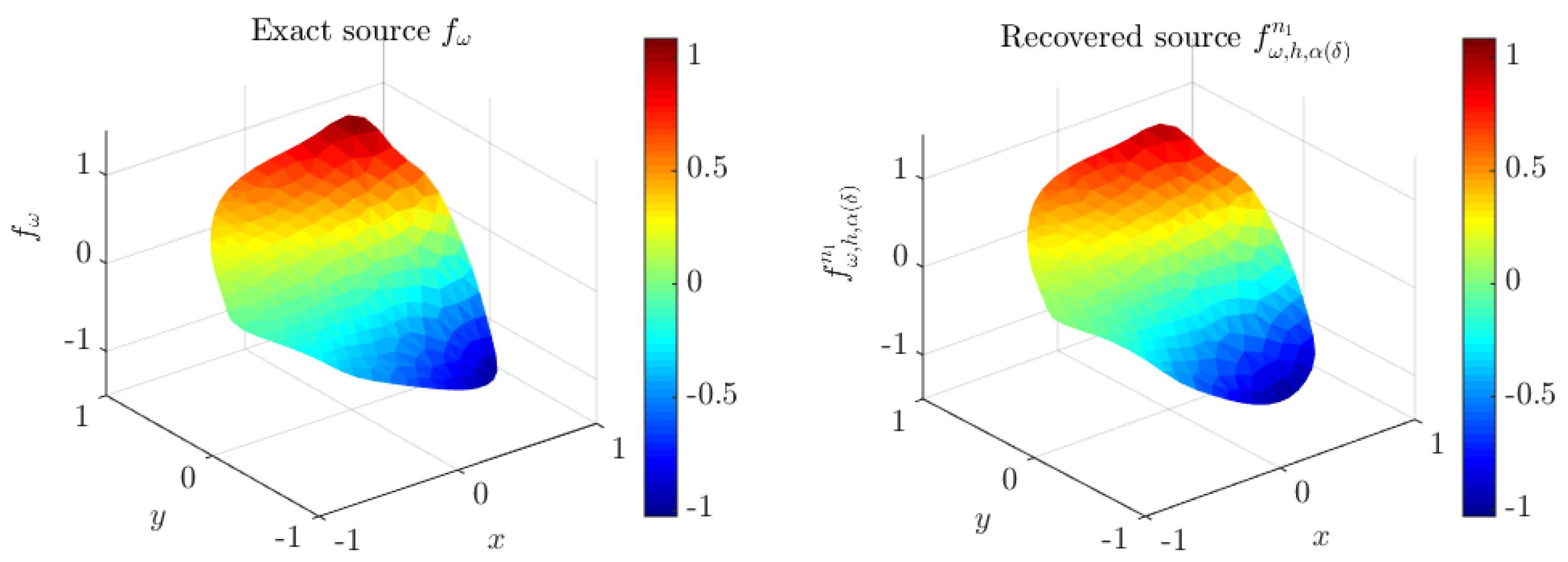
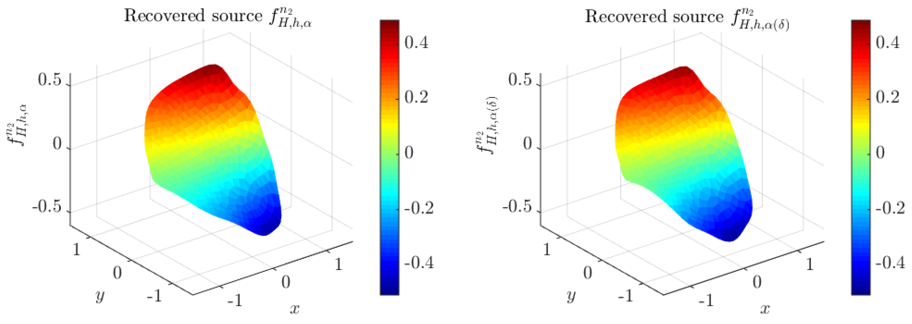
Example 4. Case when the general source is harmonic in a subdomain ω of . Let ω be a subdomain of with (see Figure 11). In this example, we are concerned with the class of sources in that are harmonic in the subdomain ω and vanish in the complement . Of course, must satisfy compatibility condition (6). We denote this particular class of harmonic sources by , which is a uniqueness class, i.e., two different functions of this class produce different measurements. Then, from (67), with , we obtain: We are interested in computing
from measurements
V on
. Since it is the subtraction of two harmonic sources,
in
and
in
, we can apply the algorithm designed to compute harmonic sources in three and two coupled regions to obtain the unique sources
and
, respectively. More precisely, we apply the Algorithm 2.
| Algorithm 2. To identify the non-harmonic component |
- Step 1.
Compute the harmonic source in from noisy data on , applying Algorithm 1 to the three coupled regions . This computed discrete source is denoted by , where is the number of conjugate gradient iterations and is the regularization parameter. - Step 2.
Compute the harmonic source in from the same noisy data, applying Algorithm 1 to the two coupled regions . This computed discrete source is denoted by , where is the number of conjugate gradient iterations and is the same regularization parameter. - Step 3.
Compute the following approximation of in :
|
We choose
and
, and the exact harmonic source
defined as in (66), but now with
slightly modified:
where
. Again, we compute the synthetic measurement
from the discrete solution
to (1)–(5), computed with the FEM using a very fine mesh
, like the one used in Example 3 of the previous Section. Additionally, the referent discrete sources
and
are computed with Algorithm 2 using this fine mesh.
Table 7 shows numerical results for noiseless data
V and noisy data
. The values shown in that table are obtained with the coarsest triangular mesh
with discretization parameter
. These results show that the numerical solutions are obtained in an stable way. We observe that all relative errors decrease when the noise of the input data decreases. Observe that the relative errors associated with the numerical calculation of
are bounded above by
for
and
, but not for
, because in this case, the discretization error dominates.
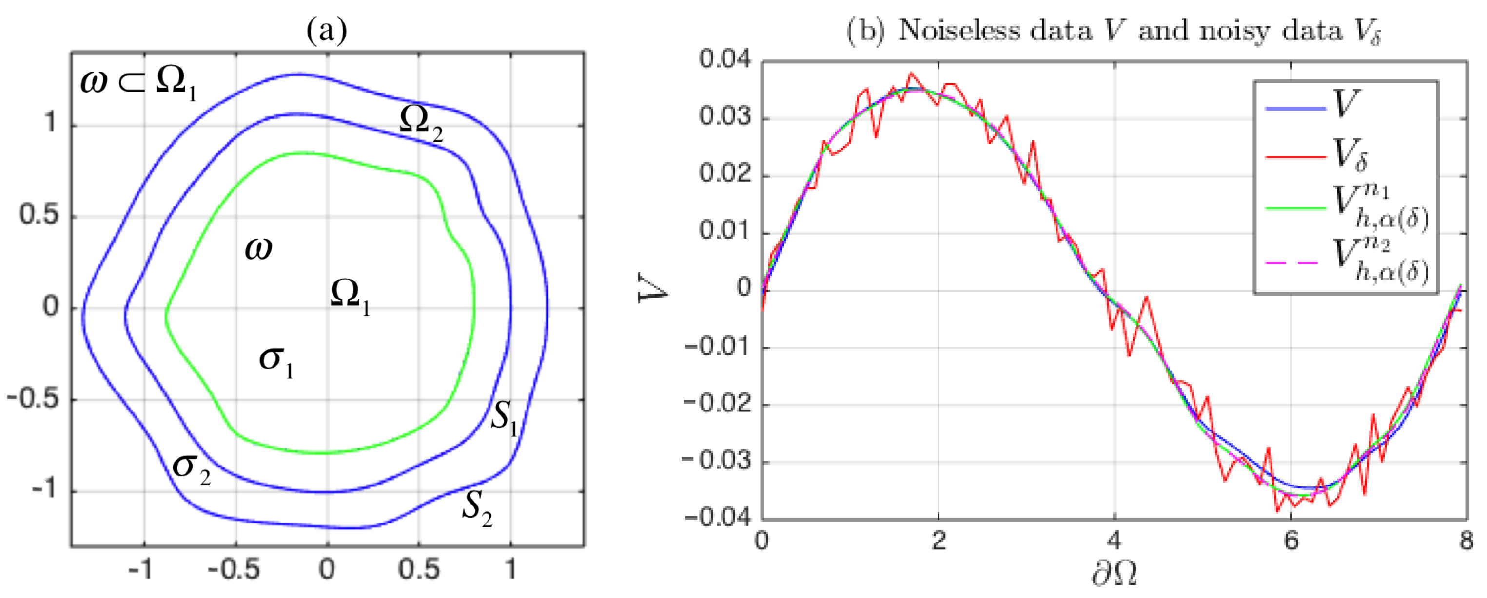
Figure 11a shows the two coupled domain and the subdomain
.
Figure 11b shows the synthetic noisy measurement
, generated by (61) with
, and the numerical potentials
,
, produced by the computed sources
and
, respectively.
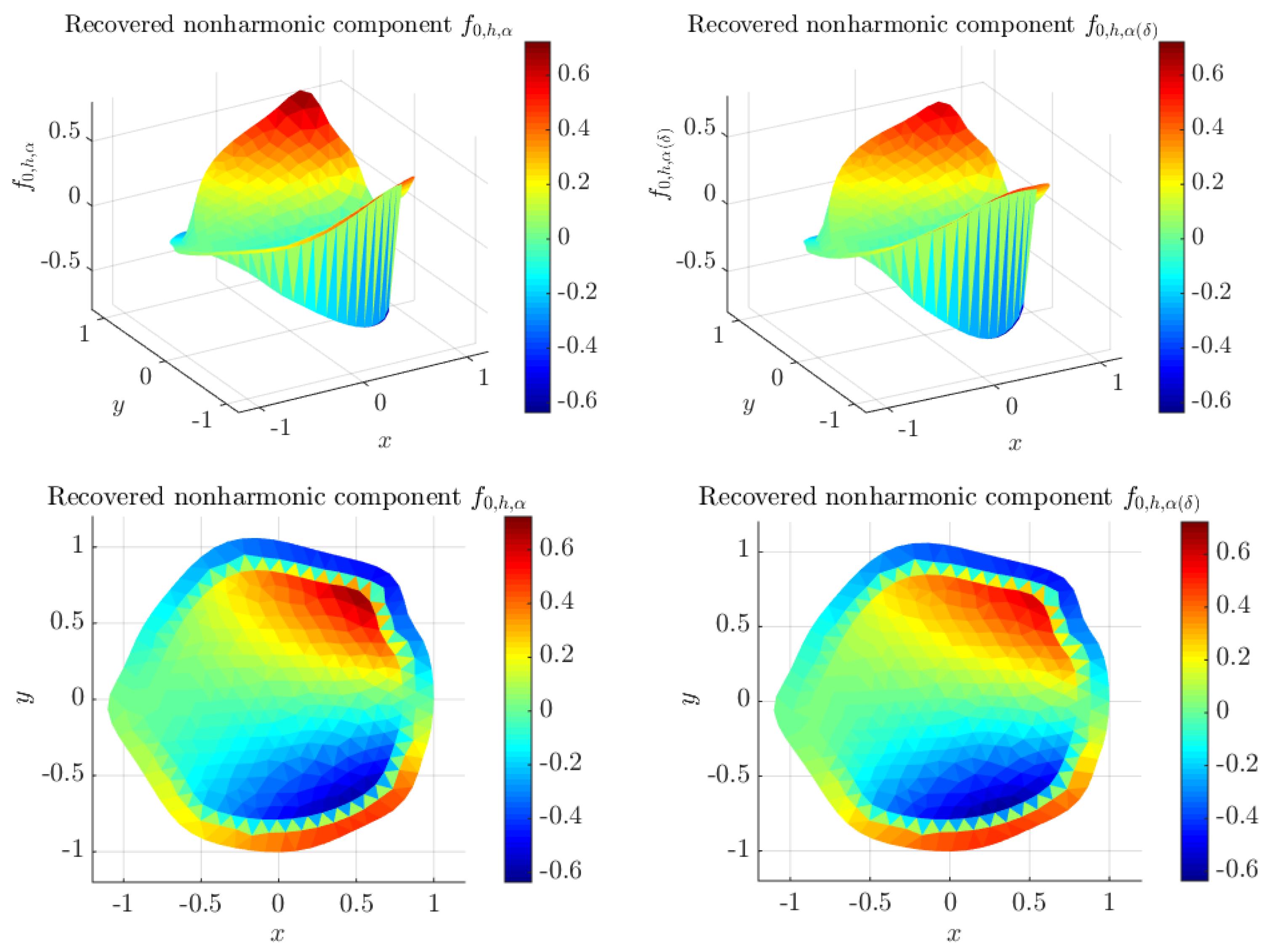
Figure 11.
(a) Irregular region with two coupled media and subdomain . The boundary of is shown in green line, and the boundaries of and , denoted by and , are shown in blue line. (b) Plots of V (blue), (red), and the recovered potentials (green) and (magenta) on , with .
Figure 11.
(a) Irregular region with two coupled media and subdomain . The boundary of is shown in green line, and the boundaries of and , denoted by and , are shown in blue line. (b) Plots of V (blue), (red), and the recovered potentials (green) and (magenta) on , with .
Figure 12,
Figure 13 and
Figure 14 show the recovered sources,
,
, and
, respectively. They are compared with to the exact solution
and the computed sources
,
, obtained from noiseless data
V.
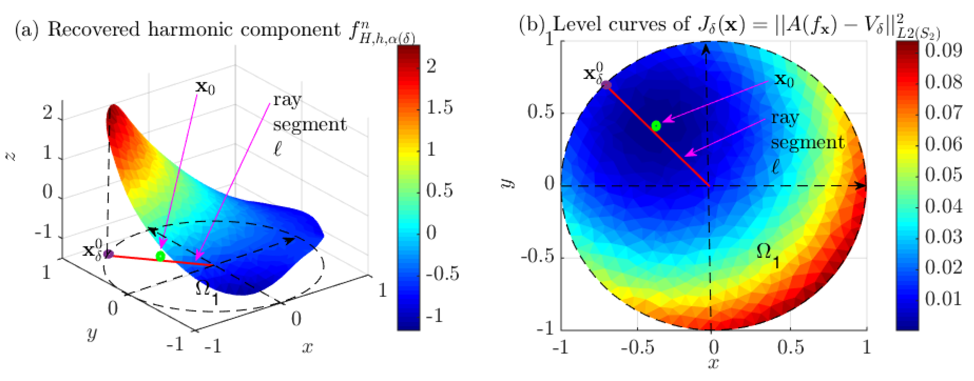
Example 5. Case of a particular class of piecewise constant sources. Let be a class of piecewise sources that take two constant values and known in , such that f takes the value in a subset and in . We consider the subclass of sources such that the sets are closed circles contained in with , where all circles ω have the same radius. Let be the center and the radius of ω. Then, each is of the formwhere is the indicator function of ω. Since must be orthogonal to the constants, we obtain Then, and , and can also be written as The set is a class of uniqueness to identify the source of the VBP (1)–(5) from a measurement V on (see Theorem 5.1 in [16]). To solve the inverse problem in a two coupled region (circular or complex) with conductivities and , we applied the Algorithm 3. | Algorithm 3. To identify a source |
- Step 1.
Find the harmonic component with Algorithm 1 (GC of Section 4) from measurements on . This computed component is denoted by . - Step 2.
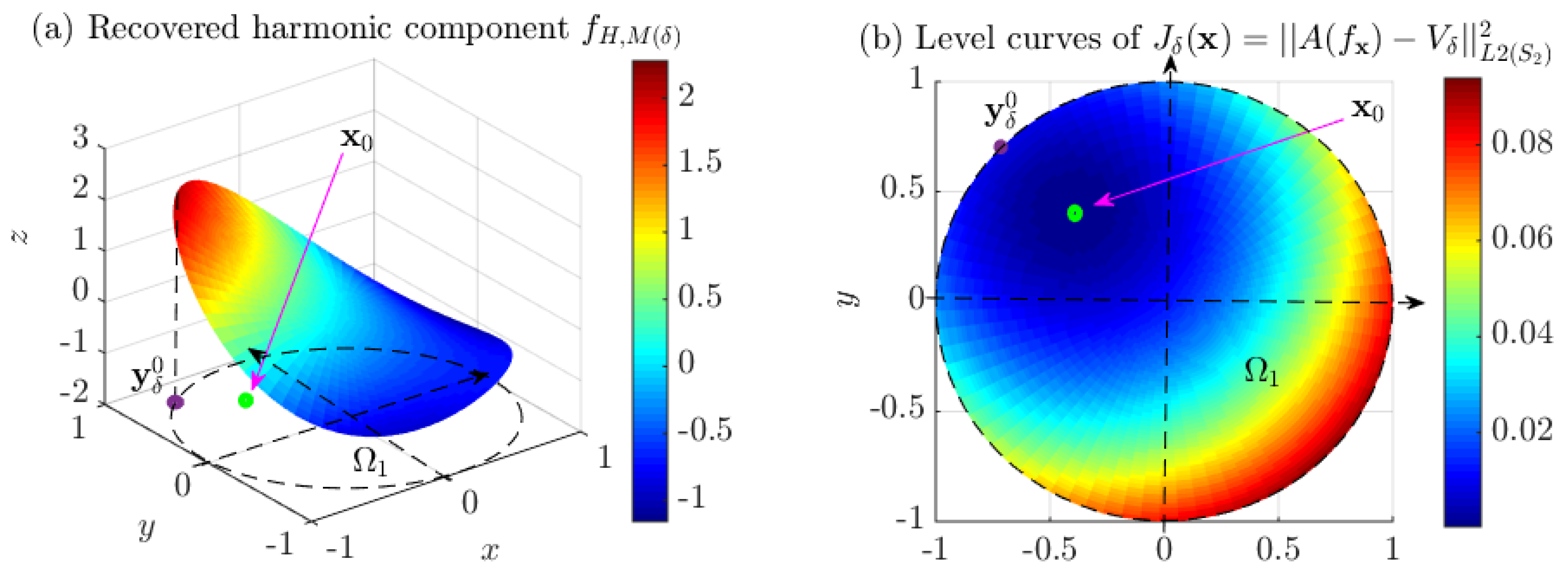
Determine the point where reaches its maximum value on (appealing to the maximum principle for harmonic functions in the bounded region ). - Step 3.
Compute the unique center of by minimizing the following convex functional:
where A is the operator defined in (17) and . Of course, also depends on the known radius of (a priori information). This computed point approximates . The minimum in Step 3 may be computed by a gradient descent method. Taking into account the geometrical characteristics of the problem (for example, see Figure 15a,b in the case of two circular coupled region ), the iterative method is designed to compute the minimum on the following ray segment:
This ray segment is guaranteed to be contained in , because . Iterative Method 3.1: Substep 3.1: Set the initial guess , with as in Step 2 above. Set the initial direction . Substep 3.2: For , if the most recent iteration point satisfies for a given fixed small tolerance , set and stop. Otherwise, update with a given step size and continue to the next substep. Substep 3.3: Update the descent direction . Do and return to Substep 3.2.
|
For circular regions, a similar algorithm is given in [
16].
Figure 15.
Case of two circular coupled region : (a) recovered harmonic component (in region ) corresponding to the exact complete source , for , obtained with Algorithm 1, which applies the finite element using a triangular mesh with a mesh size , for Method 3 presented above. (b) Level curves of the functional , where , for , and is the point in which the minimum is reached, for the Iterative Method 3.1 presented above. Similar Figures are obtained for the case of two irregular coupled regions and are not included.
We apply this algorithm with stopping parameter
and two fixed step sizes
and 0.01 to identify the source
in
for the two coupled domains shown in
Figure 16a, with conductivities
,
for
,
, respectively, where the exact set
has center
and radius
. The synthetic data are generated from the exact source (72) with
,
, and
.
Table 8 shows numerical results from noisy data
using a triangular mesh
with
. Remember that the only free parameter to completely determine
is the center
of
. These results show that the algorithm approximates the exact source
from noisy data in a stable way, since the errors
and
are bounded above by
for
and
, except for
, where the discretization error dominates. Additionally, observe that similar numerical results are obtained for the step size
, used to apply the Iterative Method 3.1.
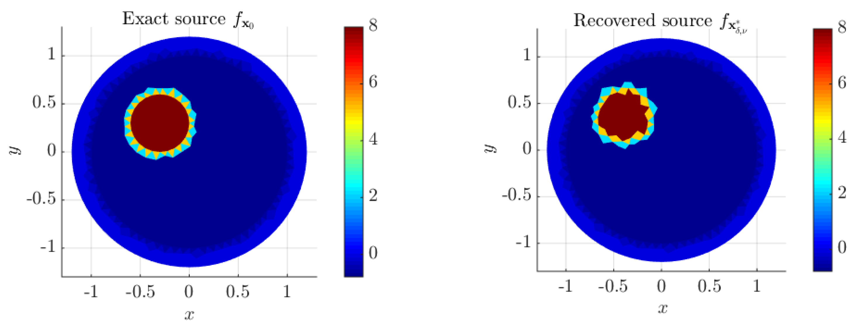
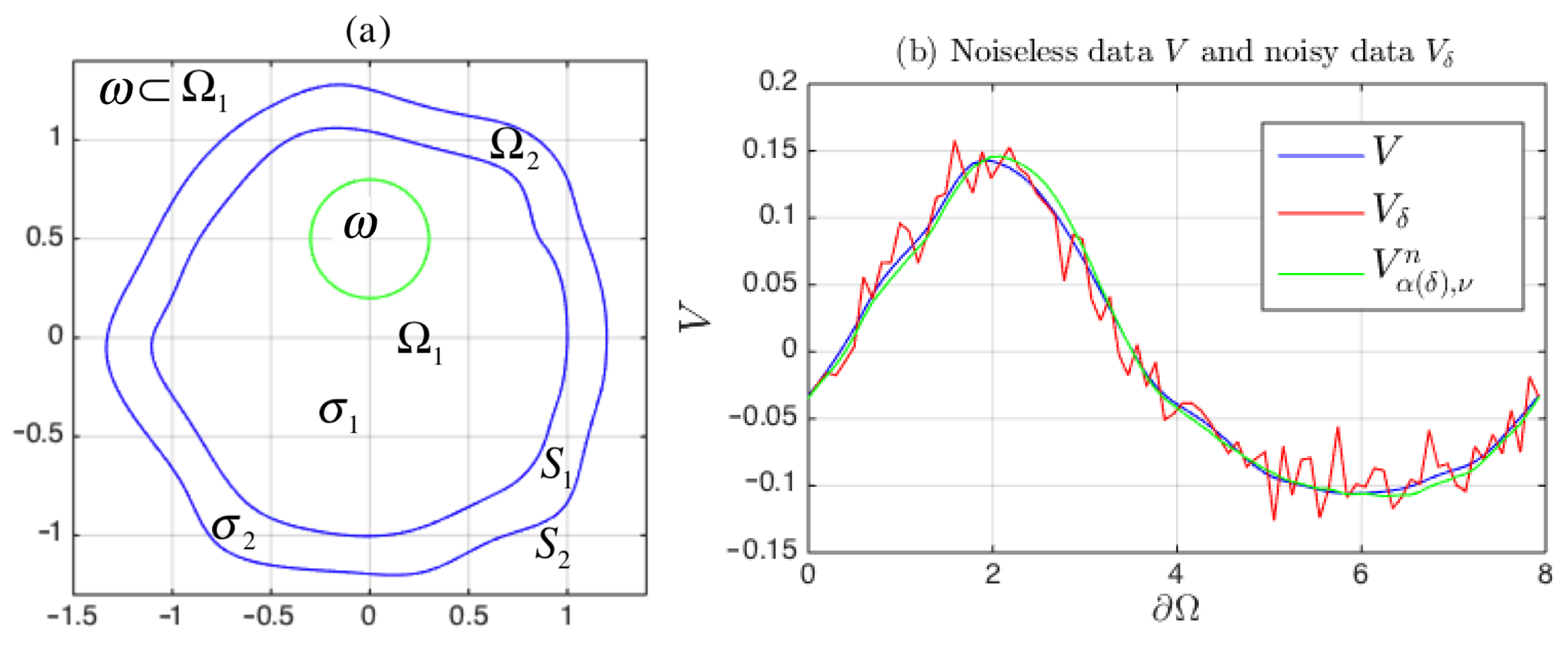
Figure 16b shows the noisy measurement
, generated by (61) with
, along with the numerical potential
generated by the recovered source
obtained with Algorithm 3 and
iterations of the Iterative Method 3.1. The exact and the numerical recovered sources are shown in
Figure 17.
Figure 16.
(a) Irregular two coupled region with the circular subdomain . The boundary of is shown in green line, and the boundaries of and , denoted by and , are shown in blue line. (b) Exact and noisy data on , V (blue) and (red), along with the recovered potential (green), for .
Figure 16.
(a) Irregular two coupled region with the circular subdomain . The boundary of is shown in green line, and the boundaries of and , denoted by and , are shown in blue line. (b) Exact and noisy data on , V (blue) and (red), along with the recovered potential (green), for .
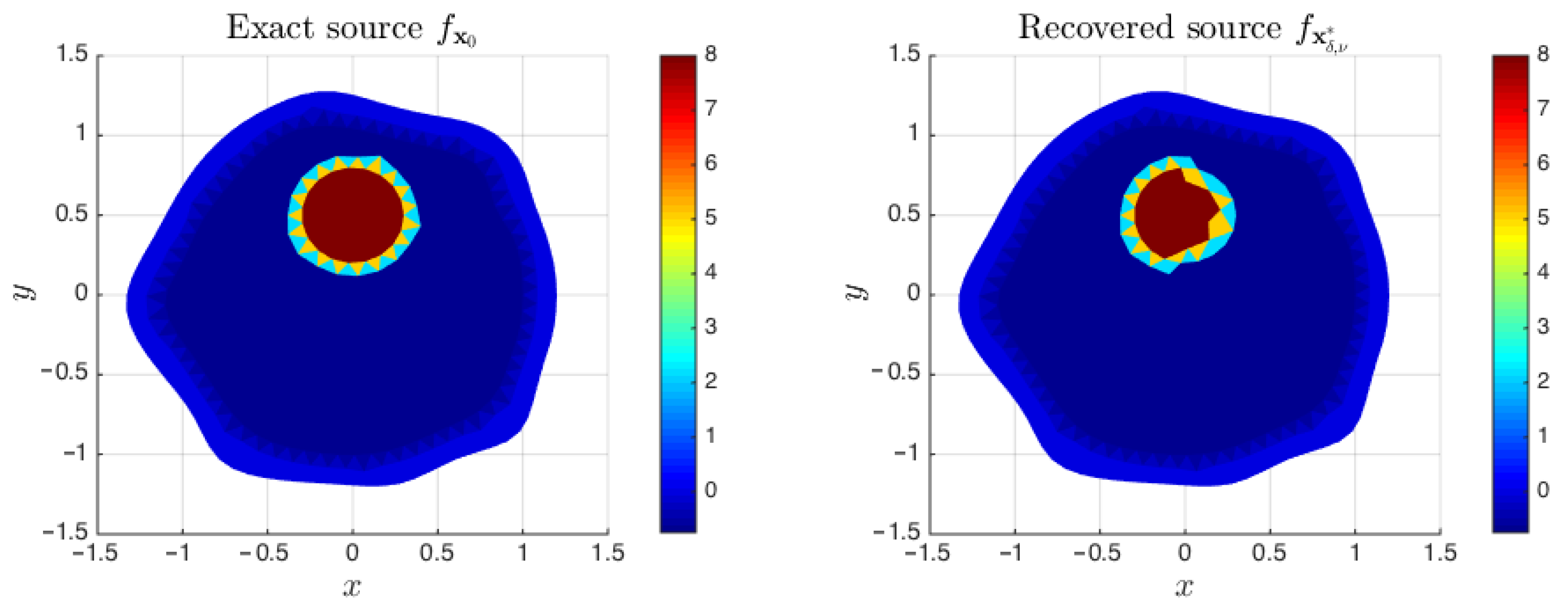
Figure 17.
Exact source and the numerical solution obtained at iteration with the Iterative Method 3.1 using mesh . Case with .
Figure 17.
Exact source and the numerical solution obtained at iteration with the Iterative Method 3.1 using mesh . Case with .
Table 8.
Numerical results obtained from noisy input data
in the region shown in
Figure 16a. The tolerance to stop the conjugate gradient iteration for both cases is
and exact source given by (72), using mesh
.
Table 8.
Numerical results obtained from noisy input data
in the region shown in
Figure 16a. The tolerance to stop the conjugate gradient iteration for both cases is
and exact source given by (72), using mesh
.
| Using Algorithm 3 with and Step Size . |
|---|
| 0 | 0.01 | 0.05 | 0.1 |
| 0 | 1.7704 | 8.7372 | 1.8427 |
| | | | |
| n (cg. iters.) | 2 | 2 | 2 | 2 |
| (−0.1356, 1.0604) | (−0.1356, 1.0604) | (−0.1356, 1.0604) | (−0.1356, 1.0604) |
| (−0.9761, 0.7628) | (−0.9761, 0.7628) | (−0.9761, 0.7628) | (−0.9761, 0.7628) |
| (number of iters.) | 12 | 12 | 12 | 11 |
| (−0.0627, 0.4900) | (−0.0627, 0.4900) | (−0.0627, 0.4900) | (−0.0658, 0.5148) |
| 4.6883 | 4.8781 | 7.7204 | 1.5390 |
| 6.3493 | 6.3493 | 6.3493 | 6.7525 |
| Using Algorithm 3 with and Step Size . |
| 0 | 0.01 | 0.05 | 0.1 |
| 0 | 1.6687 | 8.9383 | 1.4726 |
| | | | |
| n (cg. iters.) | 2 | 2 | 2 | 2 |
| (−0.1356, 1.0604) | (−0.1356, 1.0604) | (−0.1356, 1.0604) | (−0.1356, 1.0604) |
| (−0.9761, 0.7628) | (−0.9761, 0.7628) | (−0.9761, 0.7628) | (−0.9761, 0.7628) |
| (number of iters.) | 28 | 28 | 28 | 28 |
| (−0.0633, 0.4949) | (−0.0633, 0.4949) | (−0.0633, 0.4949) | (−0.0633, 0.4949) |
| 4.6883 | 4.8676 | 8.3866 | 1.1955 |
| 6.3538 | 6.3538 | 6.3538 | 6.3538 |
Example 6. Comparison with the method given in [16] for circular regions. In this example, we will compare the results obtained by applying Algorithm 3 with those obtained by applying the method introduced in [16] for the case of two coupled circular regions Ω and circular subdomains , similar to the one shown in Figure 18a. We employ the same parameter values and and the exact source defined by (72) with , , and . This time, the closed circle ω has a center at and the same radius .
The method in [
16] employs circular harmonics (a Fourier series technique) to solve both the FP and the IP using relations (53)–(60) in
Section 4.2 (in the case of two coupled circular regions
). Therefore, to numerically recover the complete source
in the circular geometry, the steps in Algorithm 3 can be simplified. For instance, in Step 1 of Algorithm 3, we may generate the harmonic component
, the solution
u to the VBP, and the synthetic data
V, employing the first
harmonics of each of the corresponding Fourier series, using polar coordinates. Then, these functions are not exact but accurate approximations. On the other hand, for the case of noisy data
, the number of Fourier terms to compute the harmonic component of the approximate source, denoted by
, depends on the level of noise (see Reference [
16]). For this example and the noise levels
,
, and
, the number of Fourier terms are
, 2, 3, respectively. In Step 2 of Algorithm 3, the MATLAB
fmincon routine may be employed to compute the point
where
takes its maximum on
(minimum of
), where only four iterations are needed (see
Figure 19a). Finally, in Step 3 of Algorithm 3, again the MATLAB
fmincon routine may be employed to find the minimum point of the functional
expressed in polar coordinates (i.e., the Iterative Method 3.1 is ignored).
Figure 19b shows the functional
expressed in Cartesian coordinates for different points
. The starting point in this minimization is denoted by
, and the minimum point is denoted by
, where
is the number of iterations conducted by
fmincon. Similar figures are obtained for the recovered harmonic component
and
when Algorithm 3 is applied (see
Figure 15a,b).
We emphasize that the numerical results obtained with the simplifications described in the previous paragraph are compared with the numerical results obtained without any simplification in the steps of Algorithm 3.
Table 9 shows the numerical results obtained with both methods for the case of noisy data
using a triangular mesh
with
. The step size when the Iterative Method 3.1 is used is
.
Therefore, as expected, the numerical results in
Table 9 show that both Algorithm 3 and the method proposed in [
16] are stable regarding noise in the input data. Additionally, the numerical results are very similar for both methods with the given discretization parameters.
Figure 18b shows the noisy data
for
, generated by (61), along with the computed potential
obtained from the recovered source
at iteration
of the Iterative Method 3.1. This figure also shows the potential
obtained from the recovered source
with the method proposed in [
16] at iteration
.
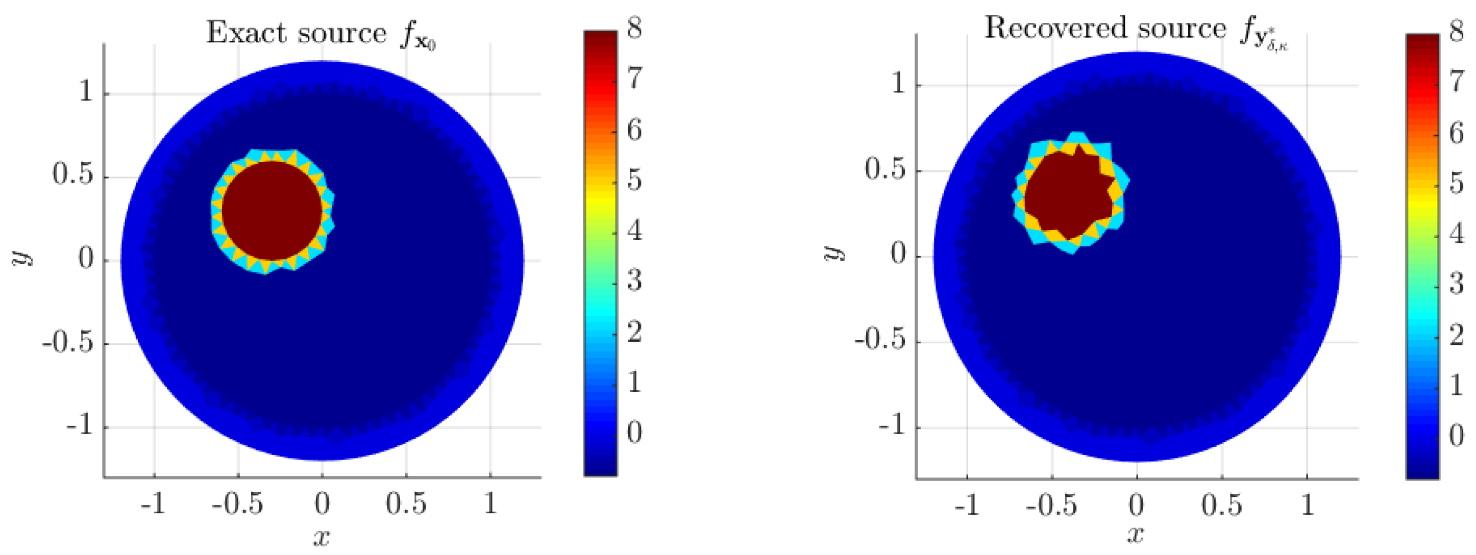
Figure 20 shows the recovered source
obtained with Algorithm 3. Finally,
Figure 21 shows the recovered source
obtained with the method proposed in [
16]. These two last Figures show that the numerical results obtained with both methods are indistinguishable.
Figure 18.
(a) Circular two coupled region with conductivities and , , and the circular subset . (b) Plots of V (blue), (red) and the two recovered potentials (green) and (magenta) on . Case with .
Figure 18.
(a) Circular two coupled region with conductivities and , , and the circular subset . (b) Plots of V (blue), (red) and the two recovered potentials (green) and (magenta) on . Case with .
Figure 19.
Case of two circular coupled region
. (
a) Recovered harmonic component
(in region
) corresponding to the exact complete source
, for
, obtained with the method given in [
16]. (
b) Level curves of the functional
, where
for
and
is the point in which the minimum is reached for the method presented in [
16].
Figure 20.
Exact source and its approximate solution at iteration of the Iterative Method 3.1. Case for using mesh .
Figure 20.
Exact source and its approximate solution at iteration of the Iterative Method 3.1. Case for using mesh .
Figure 21.
Exact source
and its approximate solution
at iteration
of the method given in [
16]. Case for
using mesh
.
Figure 21.
Exact source
and its approximate solution
at iteration
of the method given in [
16]. Case for
using mesh
.


 ,
, 
